State-Aware High-Order Diffusion Method for Edge Detection in the Wavelet Domain

Abstract

This paper addresses how to use high-order diffusion to restore the wavelet coefficients in the wavelet domain. To avoid image distortion, wavelets with symmetry are used for image decomposition to obtain the wavelet coefficients of each sub-band. Due to the influence of noise, it is particularly important to obtain the wavelet coefficients, which can accurately reflect the image information. According to the characteristics of wavelet threshold shrinkage and the advantages of the high-order variational method in denoising, a wavelet coefficient restoration scheme is proposed. The theoretical basis of our proposed method is established through the analysis of wavelet threshold theory. To keep the original structure of wavelet coefficients unchanged, we introduce the concept of state quantity of wavelet coefficients and obtain the corresponding state quantity of wavelet coefficients using normalization. The denoising wavelet coefficient is obtained by performing a fourth-order anisotropic diffusion of the state quantities. This paper takes image edge feature extraction as the experimental content and image edges are detected by the module of the wavelet coefficients. The effectiveness of the proposed algorithm is objectively verified from three aspects: denoising effect, edge continuity, and accuracy. The experimental results show that the proposed algorithm can obtain continuous and precise image edges. The algorithm presented in this paper also applies to texture images. Compared with other algorithms, the edges image obtained by this scheme shows advantages in terms of noise removal and edge protection.

1. Introduction

As a real-time image processing technology, wavelet transform and multi-scale transform based on the wavelet transform have received extensive attention [1,2,3,4]. The wavelet transform occupies an essential theoretical and practical position while it is one of the main methods used in image processing. The advantages of wavelet theory are reflected in the time-frequency and multiresolution characteristics, which can present texture and structure information at various resolution levels. In recent years, many scholars have devoted themselves to wavelet transform research and applied it to multiple aspects of image processing technology, including image denoising, image restoration, image segmentation, and edge detection [5,6,7,8,9,10,11]. Generally, an image is decomposed by wavelet transform to obtain the corresponding low-frequency and high-frequency coefficients. These coefficients reflect the details of the image, such as edges and textures. Zhang et al. used the low-frequency and high-frequency coefficient images generated by multi-wavelet transform to learn more powerful prior information, ensuring that the deep learning network provided by them can obtain better image restoration effects [10]. Based on the combination of Haar wavelet and two-dimensional discrete wavelet transform, Wang et al. proposed a watermark embedding and extraction technique for color images [11]. Making full use of the wavelet coefficients to reflect the image details is an essential factor for these methods to obtain a better processing effect. Due to the presence of noise, the critical aspect of image processing technology based on wavelets is how to obtain the wavelet coefficients that accurately reflect the information of a given image.

Wavelet shrinkage can efficiently acquire the low-frequency and high-frequency coefficients for the image with noise [12,13,14]. However, the shrinkage of wavelet coefficients makes the reconstructed image produce a pseudo-Gibbs phenomenon near the edges. To improve the application effect of wavelet transforms in image restoration, edge detection, and other technologies, it is of great practical significance to study how to obtain more wavelet transform coefficients that can accurately reflect image information.

The nonlinear diffusion methods have been widely used in image processing through partial differential equations (PDEs). Such methods use a piecewise continuous function to approximate the actual signal in an image. PDE-based denoising models mainly include second-order and high-order models (mainly fourth-order models). Examples include the total variation model [15], the Perona–Malik model [16], and anisotropic diffusion models [17,18,19,20,21,22,23]. These second-order models easily produce so-called blocky effects in the smooth regions of denoised images. Image-denoising methods based on high-order PDEs have been widely studied to overcome this shortcoming, such as the YK model [24], the LLT model [25], and the model proposed by Hajiaboli [26]. Recently, some new models have been developed [27,28,29,30,31,32]. Although high-order diffusion easily causes edge blur and makes the smooth area of an image uneven because of over-smoothness, the fourth-order models have achieved good results in removing noise and protecting edges.

This paper attempts to find a way to obtain effective wavelet coefficients and give a good theoretical explanation. First, wavelet transform is performed on the examined image to obtain the coefficients of each sub-band, and the image information mainly focuses on the high-frequency part. Due to the influence of noise, the high-frequency wavelet coefficients need to be denoised. Secondly, based on state weights, we normalize the high-frequency coefficients to obtain the corresponding continuous state weights. To eliminate the effect of noise on the high-frequency coefficients, we perform fourth-order anisotropic filtering on the state weights. Finally, by applying accurate state weights to the corresponding high-frequency wavelet coefficients, we can obtain denoised high-frequency wavelet coefficients. Because the noise is effectively suppressed, the high-frequency wavelet coefficients we obtained can not only accurately reflect the texture details of the image but also maintain the edges of the image nicely, which provides good help for the subsequent image processing method combined with wavelet transform.

This article is arranged as follows. In Section 2, we briefly introduce two methods commonly used in image denoising: wavelet shrinkage and PDE-based diffusion filtering. Section 3 describes methods for recovering wavelet coefficients that obtain an accurate reflection of image information.

This method is based on the wavelet shrinkage theory and the fourth-order anisotropic diffusion filter. In Section 4, numerical experiments are carried out, and the experimental results are analyzed from subjective and objective viewpoints. Finally, we present the conclusion of this article in Section 5.

2. Mathematical Framework

2.1. Wavelet Shrinkage Method

The wavelet shrinkage method is widely used in image restoration technology. The primary purpose of this method is to accurately find the wavelet coefficients of an image relative to the noise. The principle of the wavelet shrinkage method is to perform a wavelet transform on the studied image to obtain wavelet coefficients. The wavelet coefficients with the smaller amplitude are generated by the energy of noise, while the larger amplitudes are deemed to be generated by the energy of the signal itself. Then, an appropriate threshold value is selected to remove the noise by specifying wavelet coefficients lower than the threshold value to achieve denoising [12,13,14]. The wavelet coefficients of different sub-bands are obtained by wavelet transform so that the signal can be represented by wavelet coefficients at different scales. In practical applications, the study of the discrete wavelet transform (DWT) is of great practical significance. $f$ represents a one-dimensional signal, $\phi$ is a scaling function, and $\psi$ is a wavelet function. Given the orthogonal wavelet, the DWT is expressed as

$$f={\displaystyle \sum _{i\in Z}\langle f,{\phi }_i^n\rangle }{\phi }_i^n+{\displaystyle \sum _{j=-\infty }^n{\displaystyle \sum _{i\in z}\langle f,{\psi }_i^j\rangle }}{\psi }_i^j$$

(1)

where ${\psi }_i^j(x):=2^{-j/2}\psi (2^{-j}x-i)$ and $f\in L^2(R)$. If the signal $f$ contains Gaussian white noise, all wavelet coefficients $\langle f,{\psi }_i^j\rangle$ after the wavelet transform also contain noise, and we need to determine the effective wavelet coefficients that constitute the signal. Therefore, according to the denoising idea of the wavelet shrinkage method, the following three steps are performed to restore the original signal:

1. Analysis: A wavelet transform is applied to the noisy signal $f$, and the wavelet coefficients $d_i^j=\langle f,{\psi }_i^j\rangle$ and scaling coefficients $c_i^n=\langle f,{\phi }_i^n\rangle$ are obtained based on (1).

2. Shrinkage: Nonlinear threshold processing is performed on the wavelet coefficients by using the shrinkage function $S_{\theta }$ with a threshold parameter $\theta$, i.e., ${\tilde{d}}_i^j=S_{\theta }(d_i^j)=S_{\theta }(\langle f,{\psi }_i^j\rangle )$.

3. Synthesis: The scale coefficients are reconstructed, and the wavelet coefficients are processed by the threshold to obtain the recovered signal $u$.

$$u:={\displaystyle \sum _{i\in Z}\langle f,{\phi }_i^n\rangle }{\phi }_i^n+{\displaystyle \sum _{j=-\infty }^n{\displaystyle \sum _{i\in z}{S}_{\theta }(\langle f,{\psi }_i^j\rangle }}){\psi }_i^j$$

(2)

From (1) and (2), there are two important choices in the wavelet shrinkage method: one is the wavelet function, and the other is the threshold function. The selection of wavelet function mainly considers its symmetry, regularity, and compact support. The wavelet with symmetry, whose corresponding filter has the characteristic of linear phase, can effectively avoid phase distortion in image processing. The higher the regularity, the smoother the wavelet basis function and the more stable the reconstruction of wavelet coefficients. Moreover, the wavelet basis function with compact support has a fast convergence speed and a strong localization ability, which is beneficial to determine the abrupt point of the image. For the threshold function, if the selected threshold is small, some noise will be preserved as image information. The image will still contain more noise after denoising, and the denoising effect will not be ideal. If the selected threshold is large, although more noise can be removed, some of the detailed features in the image will also be filtered out, causing the image to blur. Therefore, the threshold needs to be determined according to the magnitude of the noise. The most commonly used shrinkage functions are hard and soft thresholding functions.

A. Hard shrinkage

$${\tilde{d}}_i^j=S_{\theta }(d_i^j)=\{\begin{array}{ll}{d}_i^j& \left|d_i^j\right|\ge \theta \\ 0& \left|d_i^j\right|<\theta \hspace{1em}\end{array}$$

(3)

B. Soft shrinkage

$${\tilde{d}}_i^j=S_{\theta }(d_i^j)=\{\begin{array}{ll}sign(d_i^j)(\left|d_i^j\right|-\theta )& \left|d_i^j\right|\ge \theta \\ 0& \left|d_i^j\right|<\theta \hspace{1em}\end{array}$$

(4)

where $\theta =\sigma \sqrt{2\ln \mathrm{N}}$, $\sigma$ is the standard deviation of the noise, and $\mathrm{N}$ is the scale or length of the signal.

2.2. PDE-Based Diffusion Method

Nonlinear diffusion has a significant influence on image processing. It utilizes a piecewise continuous function to approach the real image signal by the PDE. Unlike general linear diffusion, nonlinear diffusion not only smooths the image but also preserves its edges and details well. According to this property, many scholars have conducted extensive research on both the theoretical analysis and applications of PDEs in image processing. An anisotropic diffusion model (P-M model) introduced by Perona and Malik [16] can retain the edge features of an image by replacing the Gaussian smoothing filter with a directional heat diffusion equation. The P-M model is represented as follows.

$$\frac{\partial u}{\partial t}=div[g(\left|\nabla u\right|)\nabla u]$$

(5)

where $u$ denotes the noisy image, $t$ denotes time. $\nabla$ and $div$ represent the gradient operator and divergence operator, respectively. $g(\cdot )$ is a non-negative decreasing diffusion function. Perona and Malik provided two diffusion functions.

$$\mathrm{A}. g(\left|\nabla u\right|)=e^{-{(\left|\nabla u\right|/k)}^2} \mathrm{B}. g(\left|\nabla u\right|)=\frac{1}{1+{(\left|\nabla u\right|/k)}^2}$$

where $k$ is a parameter used to control the diffusion extension. $k$ can be pre-set or can be changed as a result of each iteration. You et al. [13] obtained the solution of (5) by minimizing the following energy function.

$$E(u)={\displaystyle {\int }_{\Omega }f(\left|\nabla u\right|)}dxdy$$

(6)

where $f(\cdot )$ is a non-negative function and $f(0)=0$. The P-M model can effectively remove noise without blurring image edges by minimizing the energy functional in (6).

An adaptive TV variational model was introduced by Strong [33] to improve the edge detection effect, as follows

$$E(u)=\underset{}{\min }{\displaystyle {\int }_{\Omega }g(x)\left|\nabla u\right|+\frac{\lambda }{2}}{\displaystyle {\int }_{\Omega }(u-u_0{)}^{2}dx}$$

(7)

where $g(x)$ is an edge-stopping function that can adaptively control the degree of diffusion. In [29], $g(x)$ is defined as

$$g(x)=\frac{1}{1+K{\left|\nabla G_{\sigma }\ast u_0\right|}^2}$$

(8)

where $G_{\sigma }$ represents the Gaussian filter and $\sigma$ is the standard deviation of the noise. Since these schemes perform diffusion faster in smooth areas, they are prone to blocky effects. To overcome this shortcoming, image restoration techniques based on high-order PDEs (especially fourth-order PDEs) have been widely studied [24,25,26,27,28,29,30,31,32]. In 2000, a classical fourth-order diffusion scheme was proposed by You and Kaveh [24], and this scheme minimizes the following functional:

$$E(u)={\displaystyle {\int }_{\Omega }f(\left|{\nabla }^{2}u\right|)}dxdy$$

(9)

where ${\nabla }^2$ denotes the Laplacian operator and $\left|{\nabla }^2\right|=\left|u_{xx}+u_{yy}\right|$. The function $f(\cdot )\ge 0$ is an increasing function. Different from the second-order diffusion model, the fourth-order model uses $\left|{\nabla }^{2}u\right|$ instead of $\left|\nabla u\right|$ to detect the smoothness of an image. Therefore, image smoothing is equivalent to finding the unique minimum value of the energy functional. The fourth-order PDE corresponding to Equation (9) can be obtained by gradient descent. The expression is depicted as

$$\frac{\partial u}{\partial t}=-{\nabla }^2[g(\left|{\nabla }^{2}u\right|){\nabla }^{2}u]$$

(10)

In 2003, Lysaker et al. proposed another classical fourth-order denoising model (LLT) [25]; the paper presented two representations of the Laplacian operator and used them as smoothing operators to process the studied images. These models can reduce image noise while relieving the staircase and blocky effects by using the Laplacian operator. However, these fourth-order PDEs easily produce speckle noise and edge blur in the restored images. Considering these issues, Hajiaboli [26] presented an anisotropic fourth-order diffusion model that performs different degrees of diffusion in the level set and gradient directions. $\xi$ and $\eta$ represent vectors in the level set direction and gradient direction, respectively. They can be expressed as

$$\xi =\frac{[-u_{y,}{u}_x]}{\left|\nabla u\right|} \eta =\frac{[u_{x,}{u}_y]}{\left|\nabla u\right|}$$

The anisotropic fourth-order diffusion formulated by Hajiaboli can be presented as

$$\frac{\partial u}{\partial t}=-{\nabla }^2(c{(\left|\nabla u\right|)}^2{u}_{\eta \eta }+c(\left|\nabla u\right|)u_{\xi \xi })$$

(11)

$u_{\eta \eta }$ is the second derivative of the image in the gradient direction. $u_{\xi \xi }$ is the second derivative in the direction orthogonal to the gradient. $c(·)$ is a diffusivity function.

$$c(\left|\nabla u\right|)=k^2/(k^2+{\left|\nabla u\right|}^2)$$

(12)

$$u_{\eta \eta }=\frac{u_x^2{u}_{xx}+u_y^2{u}_{yy}+2u_x{u}_y{u}_{xy}}{{\left|\nabla u\right|}^2} u_{\xi \xi }=\frac{u_x^2{u}_{yy}+u_y^2{u}_{xx}-2u_x{u}_y{u}_{xy}}{{\left|\nabla u\right|}^2}$$

(13)

The model performs different degrees of diffusion in different directions: in the flat region, in the directions of the gradient and the level set, the diffusion coefficients are relatively close, and at the edge of the image, the diffusion coefficient in the gradient direction is always less than the diffusion coefficient in the level set direction. Therefore, anisotropic diffusion is performed on the image. The diffusion method improves the ability of a PDE-based model to remove noise and protect the edges of the image while also leading to a relative reduction in speckle noise. However, due to the uneven diffusion of the model in the gradient direction and level set direction, the denoised image will appear uneven, reducing the image quality.

3. State-Aware Wavelet Coefficients Acquisition Method Based on Anisotropic Fourth-Order Diffusion

3.1. The Equivalent Expression of the Proposed Method

In recent years, image restoration technology combining wavelets and nonlinear diffusion has attracted much attention [34,35,36,37,38,39,40]. These methods are based on second-order diffusion in the wavelet domain. To obtain the recovered image from accurate wavelet coefficients, in this section, we present a continuous state wavelet shrinkage method based on nonlinear fourth-order diffusion. This method has a good theoretical explanation. Specifically, the main idea of our scheme is based on the two-state denoising method. Denoised wavelet coefficients are obtained by performing anisotropic diffusion on the state weights, and the wavelet coefficients can be used to further improve image restoration and edge detection.

Based on the idea of state weight, we analyze the wavelet-based hard thresholding method theoretically and give an equivalent expression for hard thresholding in the form of state weight. First, we perform discrete wavelet transform (DWT) on noisy images to obtain the wavelet coefficients $d_{j,k}$. Based on the size of the wavelet coefficients $d_{j,k}$, we determine the state of each wavelet coefficient. That is, when $\left|d_{j,k}\right|\ge \lambda$ is satisfied, the state of the wavelet coefficient is 1, while when $\left|d_{j,k}\right|<\lambda$, the state of the wavelet coefficient is set to be 0. Thus, we obtain the state quantity $v_{j,k}^{\lambda }$ corresponding to all the wavelet coefficients.

$$v_{j,k}^{\lambda }=\{\begin{array}{ll}1& \left|d_{j,k}\right|\ge \lambda \\ 0& \left|d_{j,k}\right|<\lambda \end{array}$$

(14)

where $\lambda$ is the threshold. Second, according to the state of the wavelet coefficients, the weights $w_{j,k}^{\lambda }$ can be determined.

$$w_{j,k}^{\lambda }=\{\begin{array}{ll}1& v_{j,k}^{\lambda }=1\\ 0& v_{j,k}^{\lambda }=0\end{array}$$

(15)

Finally, weights are applied to the wavelet coefficients.

$$w_{j,k}^{\lambda }(d_{j,k})=\{\begin{array}{ll}{d}_{j,k}& \left|dj,k\right|\ge \lambda \\ 0& \left|d_{j,k}\right|<\lambda \end{array}$$

(16)

The restored image is constructed by the denoised wavelet coefficients. We call the above denoising method a two-state weight denoising method, which happens to be a wavelet-based hard thresholding method. The two-state weight denoising method can remove noise well, but since there are only two states for the wavelet coefficients, which belong to the discrete state, it causes the ringing and pseudo-Gibbs phenomena. To this end, a continuous state weights denoising method is further proposed.

Since noise is mainly distributed in the high frequencies of an image, according to Section 2.1, the high-frequency subbands of the first layer after performing wavelet transform are HL subbands, LH subbands, and HH subbands, and the corresponding wavelet coefficients of these subbands are $d_{11}$, $d_{12}$, and $d_{13}$, respectively. Then, we normalize the wavelet coefficients $d_{11}$, $d_{12}$, and $d_{13}$, and the continuous state $v_{j,k}^{}$ is obtained.

$$v_{j,k}=\frac{d_{j,k}-\min d_{j,k}}{\max d_{j,k}-\min d_{j,k}}$$

(17)

In (17), on the one hand, $v_{j,k}^{}$ is obtained by the normalization of wavelet coefficients and, thus, can maintain some structural properties of the image; on the other hand, the state variables cannot be accurately estimated due to the presence of noise. Then, under the premise of maintaining the structure of the state variables, nonlinear diffusion is implemented to remove the noise effectively. Thus, more accurate state variables are obtained.

We use the diffusion method proposed by Hajiaboli to diffuse the state quantity $v_{j,k}$; here, we take $v_{1,2}$ as an example.

$$v_{1,2}\stackrel{\Delta }{=}\frac{d_{1,2}-\min d_{1,2}}{\max d_{1,2}-\min d_{1,2}}$$

(18)

The x-direction and y-direction have equal steps $\Delta x=\Delta y=1$, where $\Delta t=\tau$, $v_{i,j}^n$ is an approximation of $v_{1,2}(i,j,n\tau )$. The difference operators are given by

$$\begin{gathered} v_x\approx {\partial }_x{v}_{i,j}=(v_{i-1,j}-v_{i+1,j})/2 v_y\approx {\partial }_y{v}_{i,j}=(v_{i,j-1}-v_{i,j+1})/2 \\ {v}_{xx}\approx {\partial }_{xx}^2{v}_{i,j}=v_{i-1,j}+v_{i+1,j}-2v_{i,j} v_{yy}\approx {\partial }_{yy}^2{v}_{i,j}=v_{i,j-1}+v_{i,j+1}-2v_{i,j} \\ {v}_{xy}\approx {\partial }_{xy}^2{v}_{i,j}=(v_{i-1,j-1}+v_{i+1,j+1})/4-(v_{i-1,j+1}+v_{i+1,j-1})/4 \end{gathered}$$

Thus, the gradient magnitude can be expressed as

$${\Lambda }_{i,j}=\sqrt{{({\partial }_x{v}_{i,j})}^2+{({\partial }_y{v}_{i,j})}^2}$$

(19)

For Equation (13), ${\partial }_{\eta \eta }^2$ and ${\partial }_{\xi \xi }^2$ can be used to derive the corresponding discrete approximation expressions via the above difference operators. Utilizing Equation (11) for the diffusion of $v_{1,2}$, the difference equation is given by

$$v_{i,j}^{n+1}=v_{i,j}^n-\tau [{\partial }_{xx}^2(c{({\mathrm{\Lambda }}_{i,j}^n)}^2{\partial }_{\eta \eta }^2{v}_{i,j}^n+c({\mathrm{\Lambda }}_{i,j}^n){\partial }_{\xi \xi }^2{v}_{i,j}^n)+{\partial }_{yy}^2(c{({\mathrm{\Lambda }}_{i,j}^n)}^2{\partial }_{\eta \eta }^2{v}_{i,j}^n+c({\mathrm{\Lambda }}_{i,j}^n){\partial }_{\xi \xi }^2{v}_{i,j}^n)]$$

(20)

In this way, the noise can be removed, and the edge can be protected while a more accurate state variable ${\tilde{v}}_{j,k}$ can be obtained. Next, the value of the continuous state weight coefficients $w_{j,k}$ can be calculated according to the value of ${\tilde{v}}_{j,k}$.

$$w_{j,k}=\hspace{0.17em}{\tilde{v}}_{j,k}$$

(21)

By a similar method, the corresponding weights $w_{j,k}$ of each high-frequency sub-band are obtained for the wavelet decomposition layer. Then, by applying $w_{j,k}$ to the wavelet coefficients of the corresponding high-frequency sub-bands, the denoised wavelet coefficients are obtained, and their structure remains unchanged. The above methods can be expressed as

$${\tilde{d}}_{j,k}=w_{j,k}(d_{j,k})$$

(22)

where ${\tilde{d}}_{j,k}$ denotes the denoised wavelet coefficients.

Based on the above analysis, our proposed wavelet coefficient acquisition algorithm can be summarized as follows, where 2-scale wavelet decomposition is taken as an example.

3.2. The Implementation Steps

The steps of our proposed method are as follows:

Step 1. The noise image is decomposed by a 2-scale wavelet, and the $L{L}_{1,2}$, $L{H}_{1,2}$, $H{L}_{1,2}$, and $H{H}_{1,2}$ sub-bands are obtained.

Step 2. The high-frequency coefficients of $L{H}_{1,2}$, $H{L}_{1,2}$, and $H{H}_{1,2}$ are normalized by Equation (17) to obtain the corresponding continuous state variables $v_{j,k}^{}$.

Step 3. The fourth-order diffusion method is conducted on the state quantity $v_{j,k}^{}$ according to Equation (20).

Step 4. By using Equation (21), the weight coefficients $w_{j,k}$ are obtained as determined by ${\tilde{v}}_{j,k}$.

Step 5. By using Equation (22), $w_{j,k}$ is applied to the high-frequency wavelet coefficients.

At this point, the wavelet coefficients that remove the noise and can reflect the image features are obtained.

4. Numerical Experiments

The wavelet coefficients can better reflect the edge and detail information of the image, so we study the edge information of the image to reflect the effectiveness of the wavelet coefficients obtained by our proposed method. In this paper, the mode of the wavelet coefficients is used to get the edge information of the image. The module of the wavelet coefficients is defined as

$$Mu(x,y)={(d_{{}_{j,H}}^2+d_{{}_{j,V}}^2+d_{{}_{j,D}}^2)}^{1/2}$$

(23)

According to Section 2.1, we obtain the wavelet coefficients $d_{j,k}$ by discrete wavelet transform of the noise image $u(x,y)$, $j$ represents scale. The edge information and noise are mainly concentrated in the high-frequency subbands, thus $d_{j,H}$, $d_{j,V}$, and $d_{j,D}$ represent the horizontal, vertical, and diagonal high-frequency wavelet coefficients, respectively.

In many high-order diffusion models, the edge is detected by using the diffusion function composed of the module of the image gradient (see Equations (5) and (12)) or the module of the gradient of the image convolved with a Gaussian function (see Equation (8)). The gradient is easily disturbed by noise, which affects the detection of image edge information. We further illustrate the effectiveness of our method by comparing it with three commonly used edge detection operators, including the module of the gradient, the module of the gradient of the image convolved with a Gaussian function, and the module of the unprocessed wavelet coefficients. Canny is the most commonly used edge detection operator. In recent years, many scholars put forward many edge detection algorithms based on the Canny operator [41,42]. We select [41] for experimental verification.

This paper does experiments on images with rich texture details. We use the Figure 1 standard image for our experiments and give detailed experimental results. Daubechies (dbN) wavelet has advantages in symmetry, regularity, and compact support. At the same time, the support length of the dbN wavelet is 2N − 1, and the support length of the wavelet in most applications is generally between 5 and 9. Therefore, so we choose N = 3, namely db3 wavelet, as the wavelet base for the experiments. To obtain the initial wavelet coefficients, we use db3 to perform two-layer wavelet decomposition for the edge detection method based on the module of the wavelet coefficients. According to the following figures and tables, we compare and analyze the effects of several edge detection algorithms from the visual aspects and evaluation indicators.

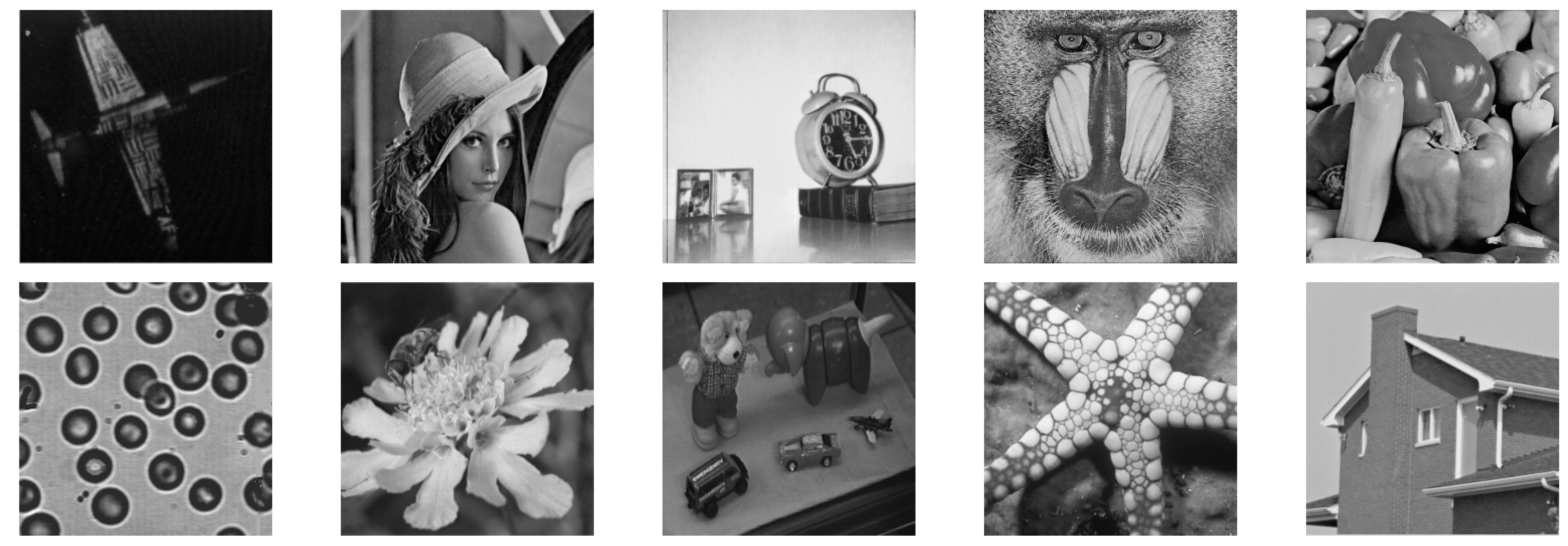
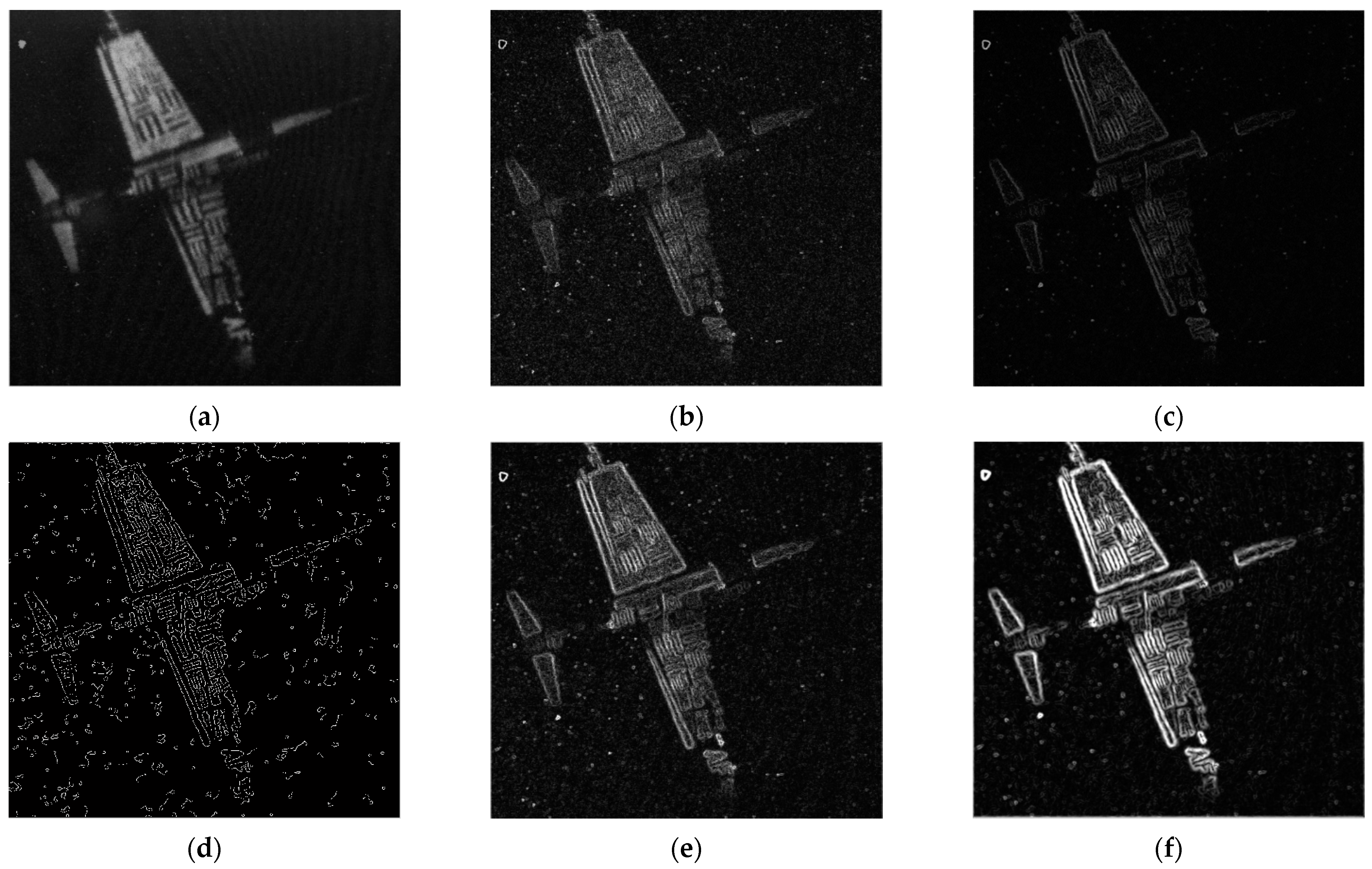
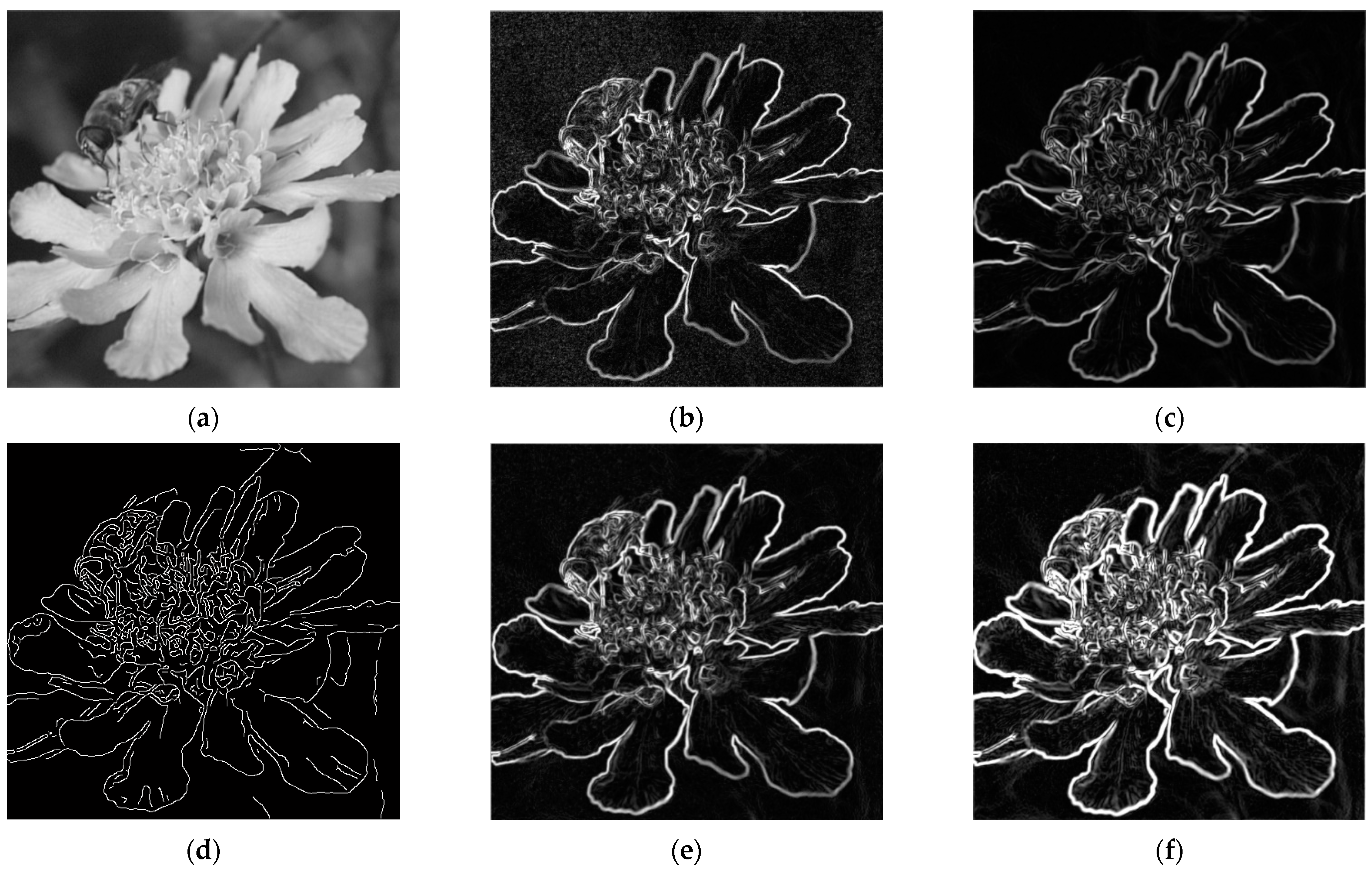
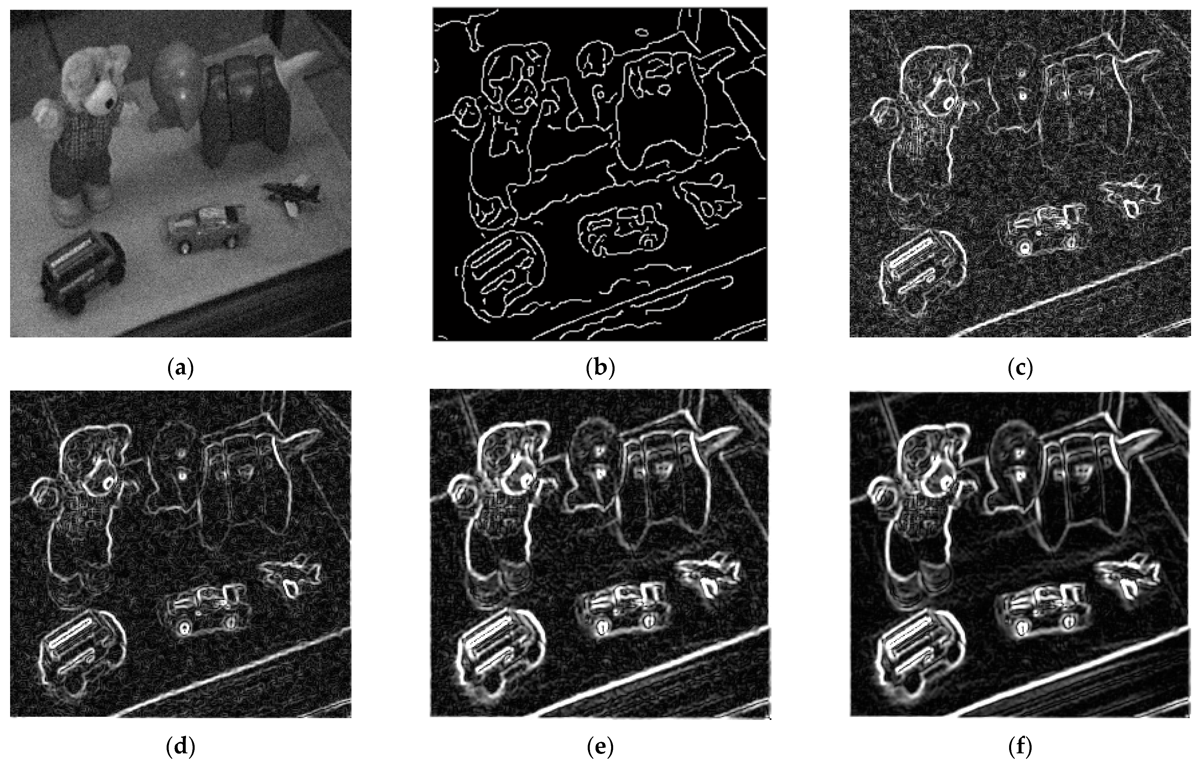
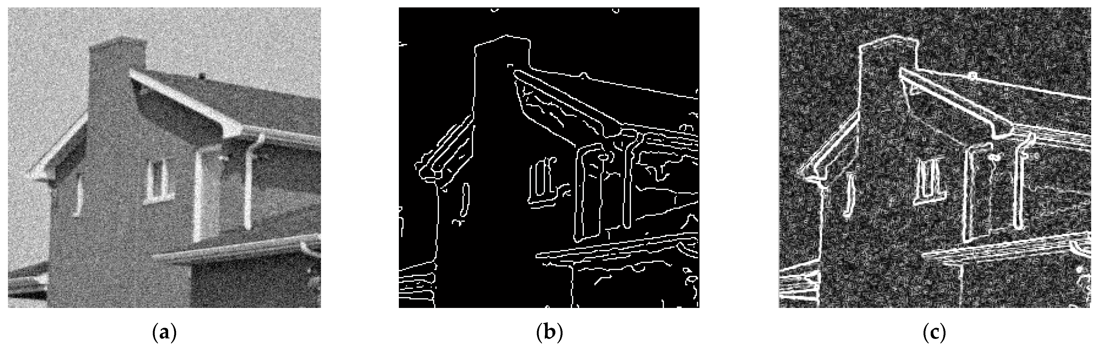
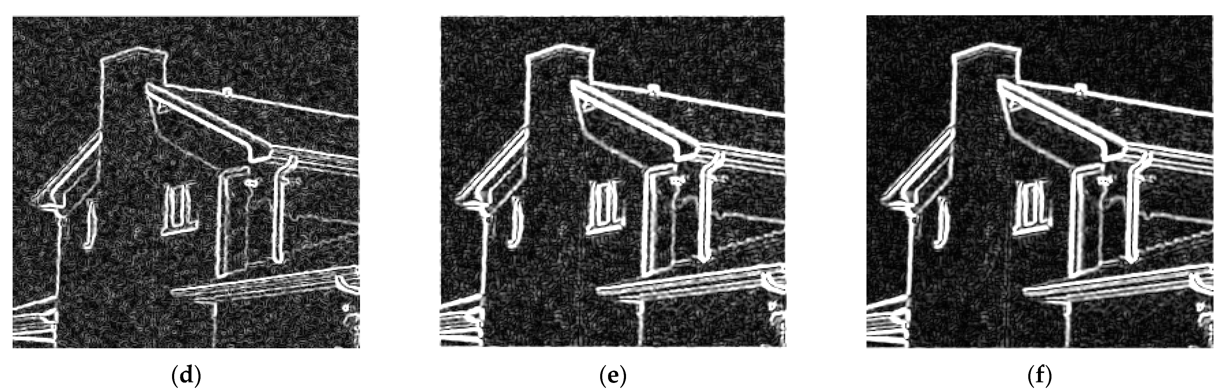
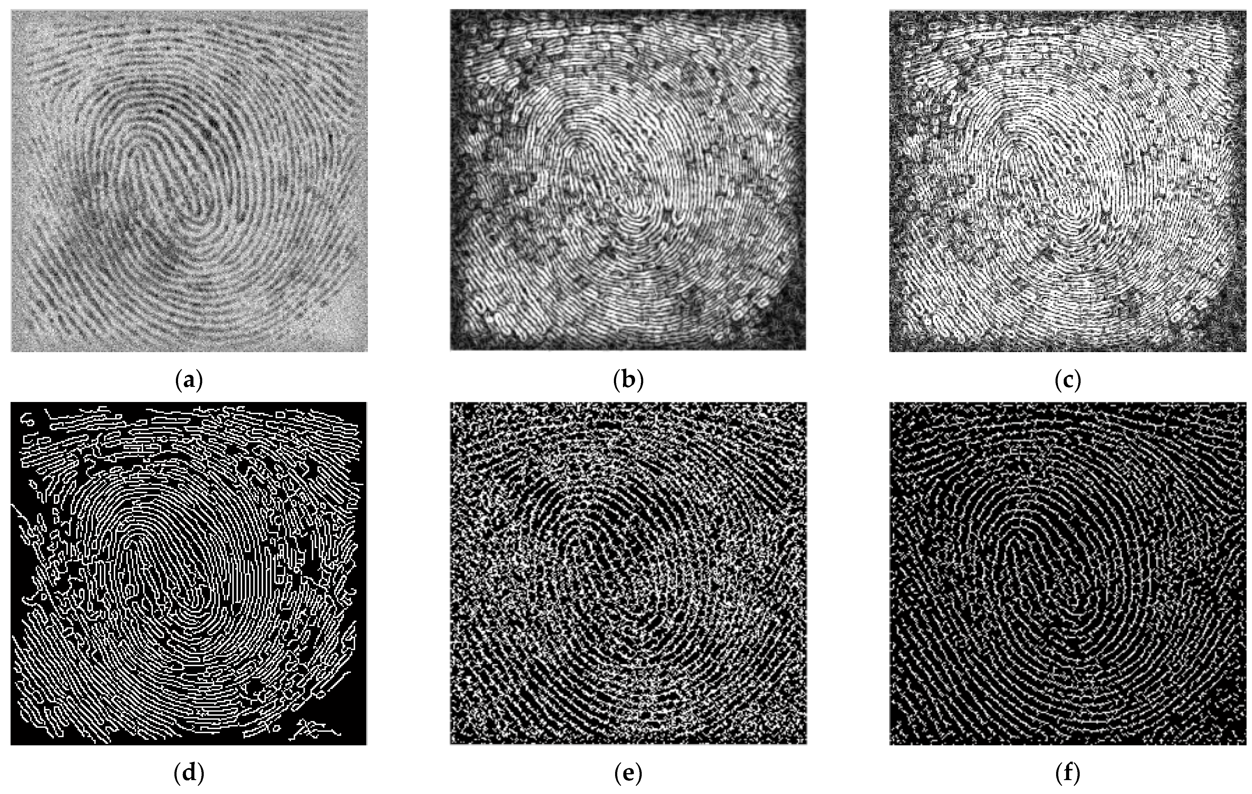
4.1. Visual Comparison

We divide the experiment into three groups. First, we perform experiments on the original acquisition images in Figure 1. Richly detailed images “airplane” and “flower” are used for the demonstration experiments, as shown in Figure 2a and Figure 3a. Figure 2b and Figure 3b show the edge detection results obtained by using the gradient detection method. The image edges or texture details detected by the gradient detection method are blurred, such as the edges of the patterns on the wings and the texture on the leaves of flowers are unclear. The experimental effect of the Gaussian smoothed gradient detection method is shown in Figure 2c and Figure 3c, where the clarity of the detected image is improved. However, the edge and texture information of the pattern is still unclear. For the [41] method, the edges of the pattern on the airplane’s wing in Figure 2d are blurred, while false edges are produced in Figure 3d, which affects the visual effect. Moreover, this method has a poor effect on texture detection. Compared with the above three methods, the detection method based on the module of the wavelet coefficients improves the display of the pattern edges and texture details. However, from the experimental results in Figure 2f and Figure 3f, we can see that our proposed method can obtain more apparent pattern edges and details, such as the lines of the pattern on the airplane wing and the texture of the petals.

Second, since most of the images we obtained contain noise, we added Gaussian white noise with standard deviations of 10 and 30 to the test images, respectively. We carry out the demonstration experiments with the images “Toys” and “house”. The “Toys” image with a standard deviation of 10 is shown in Figure 4a, and the “house” image with a standard deviation of 30 is shown in Figure 5a. For the edge detection images obtained by the [41] method, the edges of the baby elephant’s body are missing, and the texture of the bear’s clothes is not well detected in Figure 4b. In Figure 5b, there are spurious and intermittent edges in the detection results of the method described in the literature [41]; for example, the edge of the eaves is as described. Poor noise suppression and the edges of the detected image information are not clear, including the clothes of the bear in Figure 4c and the lines of the eaves in Figure 5c. The Gaussian smoothed gradient detection method suppresses the noise and improves the clarity of the edge of the image, such as the lines of the small elephant body in Figure 4d. However, the texture detection effect of the images is not good. Compared with the Gaussian smoothed gradient detection method, the detection method based on the module of the wavelet coefficients can detect more clear and more continuous image edges. Because the method does not preprocess the decomposed wavelet coefficients, the edge image still contains more noise, as shown in Figure 4e and Figure 5e. The experimental results of our proposed method are shown in Figure 4f and Figure 5f. In the detection results, we can not only see accurate and clear object edges but also see that the proposed method has an obvious noise suppression effect, and the obtained edge image has less noise and high definition. In Figure 4f, the lines and edges of the toy elephant’s body are visible.

Finally, we experiment with the texture-informative image “finger”, which contains noise when acquired, as shown in Figure 6a. As can be seen from Figure 6b,c, the gradient detection method and the Gaussian smoothed gradient detection method are greatly affected by the noise, and the detected edges are blurred. In Figure 6d, pseudo edges and intermittent edges are present in the image obtained by the [41] method. The edges obtained by the detection method based on the module of the wavelet coefficients are presented in lines, which better reflect the edge details of the original image. However, the effect of the noise suppression is not apparent, and the detection results contain noise, as shown in Figure 6e. In Figure 6f, the image detected by our proposed method has good edge continuity and accurate edge positioning, which genuinely reflects the details information of the original image. At the same time, our proposed method can effectively suppress the noise and obtain clear edge images.

4.2. Evaluation Indicators Comparison

Not only are the five edge detection operators comparable in visual effects, but the advantages of our proposed operator in edge detection can also be demonstrated objectively by the given data. In

Table 1. Comparison of PSNR (dB) for different methods on 2 levels of Gaussian noise.

Image	$\mathit{\sigma }$	Gradient Detection	Gaussian Smoothed Gradient	[41] Method	The Module of Wavelet Coefficients	Our Method
Airplane	10	30.7249	31.8325	31.3462	32.4273	32.8672
	30	27.9326	28.6239	28.1938	29.3281	29.9341
Lena	10	32.1682	32.7963	32.3252	33.5754	34.6057
	30	29.1543	29.6572	29.3836	30.3693	31.1639
Clock	10	29.7719	30.5395	30.9467	31.4836	32.3742
	30	27.3164	28.3604	28.5319	29.4625	30.5837
Baboo	10	30.8356	31.7462	31.2953	32.6931	33.7269
	30	28.7427	29.4985	29.1438	30.3438	31.5725
Peppers	10	32.4639	33.3262	33.6423	34.4716	35.3842
	30	29.4241	30.5451	30.7962	31.3932	32.4254
Cell	10	31.7396	32.6835	31.6364	33.8249	34.6028
	30	29.4037	30.2363	29.2038	31.1637	31.6546
Flower	10	30.7063	31.6307	31.2840	32.8438	33.7143
	30	28.2458	29.3352	28.8629	30.3625	31.3264
Toys	10	31.2642	31.9451	31.6672	32.8340	33.7932
	30	27.6385	28.3443	27.8957	29.1716	30.2537
Starfish	10	30.6396	31.5381	30.4852	32.4633	33.5749
	30	27.5167	28.2706	27.2178	28.9368	29.7472
House	10	32.1474	33.7206	32.5643	34.5352	35.7385
	30	26.3628	27.8583	26.9348	28.4119	29.6768
Average		29.7099	30.6245	30.1679	31.5048	32.4360

,

Table 2. Edge connectivity statistics table.

Image	Gradient Detection $\mathit{B}/\mathit{A}$	Gaussian Smoothed Gradient $\mathit{B}/\mathit{A}$	[41] Method $\mathit{B}/\mathit{A}$	The Module of Wavelet Coefficients $\mathit{B}/\mathit{A}$	Our Method $\mathit{B}/\mathit{A}$
Airplane	0.0396	0.0274	0.0529	0.0208	0.0153
Lena	0.0325	0.0291	0.0472	0.0194	0.0137
Clock	0.0421	0.0382	0.0557	0.0315	0.0263
Baboo	0.0396	0.0317	0.0469	0.0248	0.0195
Peppers	0.0268	0.0228	0.0335	0.0171	0.0120
Cell	0.0375	0.0294	0.0572	0.0269	0.0218
Flower	0.0282	0.0216	0.0394	0.0187	0.0116
Toys	0.0379	0.0325	0.0718	0.0275	0.0224
Starfish	0.0274	0.0238	0.0522	0.0182	0.0139
House	0.0395	0.0251	0.0693	0.0196	0.0127

and Table 3 the performance of the five edge detection operators is objectively compared according to the quality of the detected images.

Due to the presence of noise, the amount of noise in the obtained edge detection images can indicate the level of denoising performance of the different detection algorithms. We utilize two evaluation indicators: the mean squared error (MSE), and peak signal-to-noise ratio (PSNR). The expressions for the relevant definitions are as follows.

$$MSE(u,\overline{u})=\frac{1}{M\times N}{\displaystyle \sum _i^M{\displaystyle \sum _j^N{(u_{i,j}-{\overline{u}}_{i,j})}^2}}$$

(24)

$$PSNR=10{\log }_{10}(\frac{{255}^2}{MSE})$$

(25)

where $u$ and $\overline{u}$ are the restored image and the observed image, respectively. Here, we record the PSNR values for the second set of experimental results, as shown in Table 1.

From Table 1, the noise resistance of the five edge detection algorithms is shown. At the same noise level, the detection images acquired by the gradient detection method contain more noise and have poor noise resistance, with the lowest PSNR values obtained. This result can also be seen through the comparison of average PSNR values. The smoothing effect of the Gaussian smoothed gradient detection method improves the PSNR values. The detection method of [41] has the effect of noise suppression, but the PSNR values obtained are not as good as that of the Gaussian smoothed gradient detection method. Compared with the detection method based on the module of the wavelet coefficients, our proposed method has higher PSNR values, thus enabling the detection images to obtain more precise edges.

To further illustrate the reliability of the algorithm, the edge detection effect is evaluated using the evaluation criteria proposed in [41,42]. The evaluation criteria based on the connectivity components are given in the [41]. Where A represents the total number of detected edge points, that is, the number of pixel values of 1 in the edge image; B represents the number of edge points that meet the 8-connectivity condition. The ratio B/A can represent the edge integrity. The smaller the value, the fewer discontinuity points, the better the edge connectivity, and the higher the edge integrity. Taking the first set of experiments to obtain edge detection images as an example, we present the B/A values of their edge detection results below, as shown in Table 2. The values in Table 2 show that the ratio of our proposed algorithm B/A is smaller, with higher accuracy of edge detection and higher completeness of edge.

The quality factor is a metric proposed by Pratt to evaluate the quality of edge detection results objectively [42]. The quality factor is determined by the three factors of missed detection of true edges, misjudging noise as edges, and positioning error of edges. The general expression for the quality factor is as follows.

$$Q=\frac{1}{\max (I_a,I_b)}{\displaystyle \sum _{k=1}^{I_b}\frac{1}{1+a{d}^2(k)}}$$

(26)

where $I_a$, $I_b$, and $d$ denote the number of reference edge points, the number of detected edge points, and the vertical distance between the detected edge point and the reference edge point, respectively. $a$ is a constant factor, generally taken as 1/9. A quality factor is a positive number in the range [0, 1]. When the quality factor is larger, it means that the localization accuracy of the edge points is higher, and the accuracy of the edge detection results is better. We experiment with the edge detection results obtained for images with a noise variance of 30, and the quality factors for the various methods are shown in Table 3 below.

Table 3. Quality factor statistics table.

Image	Gradient Detection	Gaussian Smoothed Gradient	[41] Method	The Module of Wavelet Coefficients	Our Method
Airplane	0.6845	0.7251	0.5264	0.7958	0.8343
Lena	0.7364	0.7826	0.6215	0.8353	0.8736
Clock	0.6258	0.6931	0.5803	0.7238	0.7614
Baboo	0.5982	0.6348	0.5174	0.6793	0.6937
Peppers	0.6647	0.6903	0.5293	0.7218	0.7649
Cell	0.6105	0.6529	0.4937	0.6926	0.7795
Flower	0.7322	0.7851	0.6218	0.8139	0.8726
Toys	0.5937	0.6429	0.5242	0.6873	0.7284
Starfish	0.6584	0.7233	0.6149	0.7582	0.7936
House	0.6846	0.7361	0.5264	0.7843	0.8159

Table 3. Quality factor statistics table.

Image	Gradient Detection	Gaussian Smoothed Gradient	[41] Method	The Module of Wavelet Coefficients	Our Method
Airplane	0.6845	0.7251	0.5264	0.7958	0.8343
Lena	0.7364	0.7826	0.6215	0.8353	0.8736
Clock	0.6258	0.6931	0.5803	0.7238	0.7614
Baboo	0.5982	0.6348	0.5174	0.6793	0.6937
Peppers	0.6647	0.6903	0.5293	0.7218	0.7649
Cell	0.6105	0.6529	0.4937	0.6926	0.7795
Flower	0.7322	0.7851	0.6218	0.8139	0.8726
Toys	0.5937	0.6429	0.5242	0.6873	0.7284
Starfish	0.6584	0.7233	0.6149	0.7582	0.7936
House	0.6846	0.7361	0.5264	0.7843	0.8159

As can be seen from the experimental data in Table 3, the quality factor values of the edge detection results obtained by this method are higher than the quality factor values of the edge detection results obtained by the other methods. This also demonstrates the higher accuracy of the edge detection results obtained by the method in this paper.

5. Conclusions

In this paper, a wavelet coefficient recovery method combining the advantages of wavelet shrinkage and fourth-order anisotropic diffusion is proposed. The low-frequency and high-frequency wavelet coefficients are obtained by performing a discrete wavelet transform on the test images. Based on the analysis of the wavelet threshold denoising method, we propose the state-aware wavelet coefficient acquisition method, in which the focus is to obtain the state quantity corresponding to the wavelet coefficient by normalization and to conduct the fourth-order anisotropic diffusion of the state quantity. These establish the foundation for the implementation of the present method. This method avoids the direct diffusion of the wavelet coefficients and has a good theoretical interpretation. The information on image edge details can be well reflected by the module of the wavelet coefficients. The effectiveness of our proposed method is demonstrated by detecting the edge of the image. Objective experiments are based on PSNR values, B/A values (continuity judgment), and quality factor Q values (accuracy judgment). In terms of subjective vision and specific experimental data, the module of the wavelet coefficients obtained by the algorithm in this paper can accurately locate the image edges and maintain the continuity and clarity of the image edge. It provides good help for the image processing method combined with wavelet transform. The method in this paper is a real-time edge detection algorithm that plays a great role in face recognition, image segmentation, and engineering defect detection and has wide application prospects.

References

1. Donoho, D.L.; Johnstone, I.M. Wavelet Shrinkage: Asymptopia? J. R. Stat. Soc. Ser. B 1995, 57, 301–369. [Google Scholar] [CrossRef]
2. Khanna, N.; Kumar, V.; Kaushik, S.K. Wavelet packet approximation. Integral Transform. Spec. Funct. 2016, 27, 698–714. [Google Scholar] [CrossRef]
3. Khanna, N.; Kaushik, S.K. Wavelet packet approximation theorem for Hr type norm. Integral Transform. Spec. Funct. 2019, 30, 231–239. [Google Scholar] [CrossRef]
4. Guo, K.; Labate, D. Characterization and analysis of edges using the continuous Shearlet transform. SIAM J. Imaging Sci. 2009, 2, 959–986. [Google Scholar] [CrossRef]
5. Hana, R.; Foued, S. A wavelet-assisted subband denoising for tomographic image reconstruction. J. Vis. Commun. Image Represent. 2018, 55, 115–130. [Google Scholar]
6. Bayer, F.M.; Kozakevicius, A.J.; Cintra, R.J. An iterative wavelet threshold for signal denoising. Signal Process. 2019, 162, 10–20. [Google Scholar] [CrossRef]
7. Cai, X.; Wallis, C.G.; Chan, J.Y.; McEwen, J.D. Wavelet-based segmentation on the sphere. Pattern Recognit. 2020, 100, 107081. [Google Scholar] [CrossRef] [Green Version]
8. Liu, C.X.; Pang, M.Y. Automatic lung segmentation based on image decomposition and wavelet transforms. Biomed. Signal Process. Control 2020, 61, 102032. [Google Scholar] [CrossRef]
9. Kumar, A.; Saha, S.; Bhattacharya, R. Wavelet transform based novel edge detection algorithms for wideband spectrum sensing in CRNs. AEU-Int. J. Electron. Commun. 2018, 84, 100–110. [Google Scholar] [CrossRef]
10. Zhang, M.; Yang, C.; Yuan, Y.; Guan, Y.; Wang, S.; Liu, Q. multi-wavelet guided deep mean-shift prior for image restoration. Signal Process. Image Commun. 2021, 99, 116449. [Google Scholar] [CrossRef]
11. Wang, J.Y.; Du, Z.G. A method of processing color image watermarking based on the Haar wavelet. J. Vis. Commun. Image Represent. 2019, 64, 102627. [Google Scholar] [CrossRef]
12. Donoho, D.L. Denoising by soft thresholding. IEEE Trans. Inf. Theory 1995, 41, 613–627. [Google Scholar] [CrossRef] [Green Version]
13. Zhang, L.; Bao, P.; Pan, Q. Threshold analysis in wavelet based denoising. IEEE Electron. Lett. 2001, 37, 1485–1486. [Google Scholar] [CrossRef]
14. Saha, M.; Naskar, M.K.; Chatterji, B.N. Soft, hard and block thresholding techniques for denoising of mammogram image. IETE J. Res. 2015, 61, 186–191. [Google Scholar] [CrossRef]
15. Rudin, L.; Osher, S.; Fatemi, E. Nonlinear total variation-based noise removal algorithms. Physica D 1992, 60, 259–268. [Google Scholar] [CrossRef]
16. Perona, P.; Malik, J. Scale-space and edge detection using anisotropic diffusion. IEEE Trans. Pattern Anal. Mach. Intell. 1990, 12, 629–639. [Google Scholar] [CrossRef] [Green Version]
17. Zou, Q. An image inpainting model based on the mixture of Perona-Malik equation and Cahn-Hilliard equation. J. Appl. Math. Comput. 2021, 66, 21–38. [Google Scholar] [CrossRef]
18. Lou, Y.; Zeng, T.; Osher, S.; Xin, J. A weighted difference of anisotropic and isotropic total variation model for image processing. SIAM J. Imaging Sci. 2015, 8, 1798–1823. [Google Scholar] [CrossRef] [Green Version]
19. Shama, M.-G.; Huang, T.-Z.; Liu, J.; Wang, S. A convex total generalized variation regularized model for multiplicative noise and blur removal. J. Appl. Math. Comput. 2016, 276, 109–121. [Google Scholar] [CrossRef]
20. Hsieh, P.-W.; Shao, P.-C.; Yang, S.-Y. A regularization model with adaptive diffusivity for variational image denoising. Signal Process. 2018, 149, 214–228. [Google Scholar] [CrossRef]
21. Pang, Z.-F.; Zhou, Y.-M.; Wu, T.; Li, D.-J. Image denoising via a new anisotropic total variation-based model. Signal Process. Image Commun. 2019, 74, 140–152. [Google Scholar] [CrossRef]
22. Lv, Y.H. Total generalized variation denoising of speckled images using a primal-dual algorithm. J. Appl. Math. Comput. 2020, 62, 489–509. [Google Scholar] [CrossRef]
23. Chen, Y.; He, T.S. Image denoising via an adaptive weighted anisotropic diffusion. Multidimens. Syst. Signal Process. 2021, 32, 651–669. [Google Scholar] [CrossRef]
24. You, Y.L.; Kaveh, M. Fourth-order partial differential equation for noise removal. IEEE Trans. Image Process. 2000, 9, 1723–1730. [Google Scholar] [CrossRef] [Green Version]
25. Lysaker, M.; Lundervold, A.; Tai, X.C. Noise removal using fourth-order partial differential equation with applications to medical magnetic resonance image in space and time. IEEE Trans. Image Process. 2003, 12, 1579–1590. [Google Scholar] [CrossRef]
26. Hajiaboli, M.R. An anisotropic fourth-order nonlinear diffusion filter for image noise removal. Int. J. Comput. Vis. 2011, 92, 177–191. [Google Scholar] [CrossRef]
27. Shi, B.L.; Pang, Z.F.; Yang, Y.F. A projection method based on the splitting Bregman iteration for the image denoising. J. Appl. Math. Comput. 2012, 39, 533–550. [Google Scholar] [CrossRef]
28. Zhang, X.J.; Ye, W.Z. An adaptive fourth-order partial differential equation for image denoising. Comput. Math. Appl. 2017, 74, 2529–2545. [Google Scholar] [CrossRef]
29. Siddig, A.; Guo, Z.; Zhou, Z.; Wu, B. An image denoising model based on a fourth-order nonlinear partial differential equation. Comput. Math. Appl. 2018, 76, 1056–1074. [Google Scholar] [CrossRef]
30. Yang, J.H.; Zhao, X.L.; Mei, J.J. Total variation and high-order total variation adaptive model for restoring blurred images with Cauchy noise. Comput. Math. Appl. 2019, 77, 1255–1272. [Google Scholar] [CrossRef]
31. Deng, L.; Zhu, H.; Yang, Z.; Li, Y. Hessian matrix-based fourth-order anisotropic diffusion filter for image denoising. Opt. Laser Technol. 2019, 110, 184–190. [Google Scholar] [CrossRef]
32. Chen, Y.; Gao, Y. Adaptive fourth-order diffusion smoothing via bilateral kernel. Signal Image Video Process. 2021, 15, 1125–1133. [Google Scholar] [CrossRef]
33. Strong, D.M. Adaptive Total Variation Minimizing Image Restoration; UCLA CAM Report97-38. Ph.D. Thesis, University of California, Los Angeles, CA, USA, 1997. [Google Scholar]
34. Cai, J.F.; Dong, B.; Osher, S.; Shen, Z. Image restoration: Total variation, wavelet frames, and beyond. J. Am. Math. Soc. 2012, 25, 1033–1089. [Google Scholar] [CrossRef] [Green Version]
35. Xu, J.T.; Jia, Y.Y.; Shi, Z.F. An improved anisotropic diffusion filter with semi-adaptive threshold for edge preservation. Signal Process. 2016, 119, 80–91. [Google Scholar] [CrossRef]
36. Shen, Y.; Liu, Q.; Lou, S.Q.; Hou, Y.L. Wavelet-Based Total Variation and Nonlocal Similarity Model for Image Denoising. IEEE Signal Process. Lett. 2017, 24, 877–881. [Google Scholar] [CrossRef]
37. Dong, B.; Jiang, Q.T.; Shen, Z.W. Image restoration: Wavelet frame shrinkage, nonlinear evolution PDEs, and Beyond. Multiscale Model. Simul. 2017, 15, 606–660. [Google Scholar] [CrossRef] [Green Version]
38. Xiang, R.; Wang, L.; He, Q. Image denoising algorithm based on wavelet transform and partial differential equations. Commun. Technol. 2017, 50, 30–37. [Google Scholar]
39. Tanyeri, U.; Demirci, R. Wavelet-Based Adaptive Anisotropic Diffusion Filter. Adv. Electr. Comput. Eng. 2018, 18, 99–106. [Google Scholar] [CrossRef]
40. Wang, J.; Yang, C.L. An improved image denoising model based on partial differential equation in wavelet domain. Comput. Technol. Autom. 2018, 37, 95–98. [Google Scholar]
41. Yu, X.K.; Wang, Z.W.; Wang, Y.H.; Zhang, C.L. Edge Detection of Agricultural Products based on Morphologically Improved Canny Algorithm. Math. Probl. Eng. 2021, 2021, 6664970. [Google Scholar] [CrossRef]
42. You, N.; Han, L.B.; Zhu, D.M.; Song, W.W. Research on image denoising in edge detection based on wavelet transform. Appl. Sci. 2023, 13, 1837. [Google Scholar] [CrossRef]
Figure 1. Testing images. The first row: Airplane, Lena, Clock, Baboo, and Peppers; the second row: Cell, Flower, Toys, Starfish, and House.
Symmetry 15 00803 g001
Figure 2. Results of edge detection obtained with the “airplane” image by using five methods: (a) original image, (b) the gradient detection method, (c) Gaussian smoothed gradient detection method, (d) [41] method, (e) the module of the wavelet coefficient detection method, (f) our proposed method.
Symmetry 15 00803 g002
Figure 3. Results of edge detection obtained with the “flower” image by using five methods: (a) original image, (b) gradient detection method, (c) Gaussian smoothed gradient detection method, (d) [41] method, (e) the module of the wavelet coefficient detection method, (f) our proposed method.
Symmetry 15 00803 g003
Figure 4. Results of edge detection obtained with “Toys” image by using four methods: (a) noisy image ( σ = 10 ), (b) [41] method, (c) gradient detection method, (d) Gaussian smoothed gradient detection method, (e) the module of the wavelet coefficient detection method, (f) our proposed method.
Symmetry 15 00803 g004
Figure 5. Results of edge detection obtained with the “House” image by using four methods: (a) noisy image ( σ = 30 ), (b) [41] method, (c) gradient detection method, (d) Gaussian smoothed gradient detection method, (e) the module of the wavelet coefficient detection method, (f) our proposed method.
Symmetry 15 00803 g005aSymmetry 15 00803 g005b
Figure 6. Results of edge detection obtained with the “finger” image by using five methods: (a) original image, (b) gradient detection method, (c) Gaussian smoothed gradient detection method, (d) [41] method, (e) the module of the wavelet coefficient detection method, (f) our proposed method.
Symmetry 15 00803 g006