Abstract
Shannon developed the idea of entropy in 1948, which relates to the measure of uncertainty associated with a random variable X. The contribution of the extropy function as a dual complement of entropy is one of the key modern results based on Shannon’s work. In order to develop the inferential aspects of the extropy function, this paper proposes a non-parametric kernel type estimator as a new method of measuring uncertainty. Here, the observations are exhibiting -mixing dependence. Asymptotic properties of the estimator are proved under appropriate regularity conditions. For comparison’s sake, a simple non-parametric estimator is proposed, and in this respect, the performance of the estimator is investigated using a Monte Carlo simulation study based on mean-squared error and using two real-life data.
1. Introduction
Reference [1] made a significant contribution to statistics by coining the term “entropy”, which refers to the measurement of uncertainty in a probability distribution. If X is a non-negative random variable (rv) that admits an absolutely continuous cumulative distribution function (cdf) with the corresponding probability density function (pdf) , then the Shannon entropy concept associated with X can be defined as follows:
Previous research explores numerous extended and generalized versions of Shannon’s entropy function. Indeed, an excellent review of various developments on Shannon’s entropy function and its inferential aspects is covered by [2].
One of the main contemporary findings based on Shannon’s work is the contribution of a study by [3], which suggests the extropy function as a dual complement of entropy. It is defined for an absolutely continuous and non-negative rv X with pdf as the following:
It is evident from Equation (2) that J(X) < 0, and hence extropy, in contrast to entropy, is always negative. The research by [3] notes that a binary distribution’s entropy and extropy are equal and as in the case of entropy, the maximum extropy distribution is the uniform distribution. Following on from the work of [3] the study of extropy has increased considerably both from a theoretical and applied point of view. Reference [4] made a comparison with extropy and some existing measures of uncertainty available in the literature and showed that there are situations where extropy can be utilized to deliver more information than those measures of uncertainty. One of the main statistical application of extropy is the total log scoring rule, which is used to score the forecasting distributions. In the application point of view, the use of extropy in automatic speech recognition was given by [5]. One can refer to [6] for the application of extropy in thermodynamics and statistical mechanics. Reference [7] explored some properties of it, involving some characterization results using order statistics and record values. Several works are available in the literature related to the inferential aspect of extropy function based on independent observations. Reference [8] proposed the development of extropy estimators in applications for testing uniformity and also used extropy to compare the uncertainties of two rvs. A study by [9] provided kernel estimation of extropy function under length-biased sampling. More recently, Reference [10] developed non-parametric log kernel estimator of extropy function.
In practice, it seems more realistic to drop the idea of independence, and replace it with some mode of dependence. However, in the case of extropy function, no inferential aspects have been proposed in previous research based on dependent data. With this in mind, the goal of this current research is to propose a non-parametric estimator of extropy function that relies on recursive kernel type estimation based on dependent data. Even various mixing conditions are available in the literature; -mixing is the better mixing condition and has many applications (see, Reference [11]), which motivates us to estimate extropy function under -mixing dependence condition. Unlike other research relating to recursive estimation, this paper develops a detailed analysis on recursive kernel estimation using simulation and time series data.
Let be a probability space and be the -algebra of events obtained by the rvs . The stationary process is said to satisfy the -mixing (strong mixing) condition if
as . This implies that as m approaches infinity, then the rvs and become asymptotically independent. Here, the coefficient is known as the mixing coefficient.
Previous researchers in the field have studied non-parametric estimation for dependent data. These investigations include the non-parametric kernel type estimation of past extropy, and residual extropy, under -mixing dependence condition (see, References [12,13]). Reference [14] developed non-parametric kernel type estimators for Mathai-Haubold entropy and its residual version based on -mixing dependent data. Furthermore, a study by Reference [15] explores the recursive and non-recursive kernel estimation of negative cumulative residual extropy under -mixing dependence condition.
This current paper adopts the following structure: Section 2 explores non-parametric recursive kernel estimator for the extropy function, while Section 3 presents the asymptotic properties of the proposed estimator. Section 4 outlines a simulation study in order to illustrate the performance of the proposed estimator. Section 5 discusses how the application of the estimator to real-life data is implemented. Finally, Section 6 provides a conclusion with some future aspects.
2. Estimation of Extropy Function
In this section, the idea for the development of a non-parametric recursive kernel estimator for the extropy function will be proposed. The main feature of recursive density estimators in comparison with non-recursive estimators is that they can be updated with each additional observation. In the case of non-recursive estimators, they must be entirely recomputed.
Let be a sequence of identically distributed rvs representing the life-times for n components. Here, the life-times are assumed to be -mixing. The assumptions are made in the study by [16]. Reference [17] is used for deriving the asymptotic properties of the estimator and for the purpose of comparison, the definition of a simple non-parametric estimator of can be given as follows:
where
This represents the kernel estimator obtained from the sample without (see, Reference [18]).
Following on from this, the non-parametric recursive kernel estimator for is:
where is a non-parametric estimator of density function.
However, the mostly used non-parametric recursive estimator of is the kernel estimator (see, Reference [19]), which is given as:
where satisfies the conditions: is bounded, non-negative, symmetric, , , and is a sequence of positive bandwidths such that and as , and .
Under -mixing dependence condition, the expressions for the bias and variance of are outlined by (see, Reference [16]):
and
where , is the derivative of the pdf and .
3. Recursive Property and Asymptotic Results
This section supports that the proposed estimator exhibits a recursive property and the asymptotic results of the corresponding estimator are shown here.
Theorem 1.
Let be a non-parametric estimator of as defined in Equation (6). Then, it meets the recursive property:
Proof of Theorem 1.
We have,
and
here,
then, we get
The result of rearranging the equation above is Equation (10). Hence, the theorem is proved. □
Theorem 2.
Let be a kernel of order s and let be a sequence of numbers that satisfies the conditions given in Section 2. Then, is a consistent estimator of , that is
Proof of Theorem 2.
By using Taylor’s series expansion, we have
Hence, the expressions for the bias, variance and mean-squared error () of are, respectively,
and
From Equation (19), as , .
Therefore,
Thus, the theorem is proved. □
Remark 1.
The bias and variance of the estimator is obtained as
and
Theorem 3.
Suppose is a non-parametric estimator of as defined in Equation (6). Then, is integratedly consistent in quadratic mean estimator of .
Proof of Theorem 3.
(Proof of Theorem 3). Consider the mean integrated square error of denoted as . Then,
Theorem 4.
Proof of Theorem 4.
We have
By using the asymptotic normality of given in Reference [16], we can conclude that
has N(0,1) as with given in Equation (26). Hence, the theorem results. □
4. Monte Carlo Simulation
A simulation study is carried out to compare the kernel estimator and in terms of the . In the first case, is generated from the exponential AR(1) process with correlation coefficient = 0.2 and parameter . The Gaussian kernel is used as the kernel function for the estimation. The estimated value, bias and of and for various sample sizes (n) 10, 20, 50, 100, 150, 200, 250, 300, 350, 400, 450, 500 and these values are calculated in the case of the exponential AR(1) process, as shown in Table 1 and Table 2.

Table 1.
Exponential AR(1), Estimated value (E), Bias and of with = 0.375.
Table 2.
Exponential AR(1), E, Bias and MSE of with = 0.375.
From Table 1 and Table 2, it can be seen that the proposed estimate for the extropy function performs better than the estimate based on the obtained MSE.
Furthermore, Gaussian distribution with parameters = 5 and = 3 is considered, from which is generated for constructing the Gaussian AR(1) process with correlation coefficient = 0.5. The estimation is conducted using the Gaussian kernel function. The bias and MSE of and for various sample sizes 10, 20, 50, 100, 150, 200, 250, 300, 350, 400, 450 and 500 are calculated for the Gaussian AR(1) process, as shown in Table 3 and Table 4.
Table 3.
Gaussian AR(1), E, Bias and MSE of with = 0.0399.
Table 4.
Gaussian AR(1), E, Bias and MSE of with = 0.0399.
Table 3 and Table 4 show that the proposed estimate for the extropy function is better than the estimate based on the MSE. All simulations were executed using R programming language with standard computation time. Moreover, R-code to find by simulation for size n = 50 is given in the Appendix A.
5. Data Analysis
5.1. Application 1
For the first application, time series data relating to International Airline Passengers: Monthly Totals from January 1949 to December 1960 (comprising thousands of passengers) are considered for analysis. This time series data are also used in a study by [21]. The time series plot, sample auto correlation function (ACF) and partial autocorrelation function (PACF) plot of the data are shown in Figure 1, Figure 2 and Figure 3.
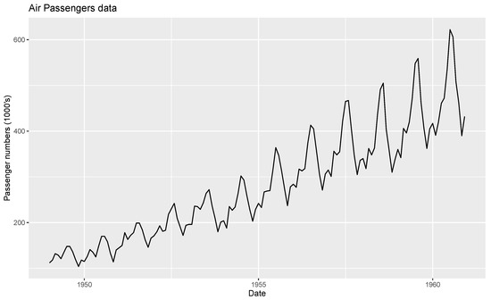
Figure 1.
Time series plot of monthly totals of International Airline Passengers data.
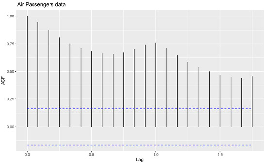
Figure 2.
ACF plot of monthly totals of International Airline Passengers data.
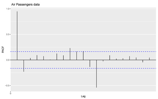
Figure 3.
PACF plot of the data monthly totals of International Airline Passengers.
From Figure 1, Figure 2 and Figure 3, the data show random components, seasonality, and trends. The time series data are decomposed in order to arrive at estimates of trends, seasonal and random components, using the moving average method. Figure 4 shows the decomposition of the time series data into trends, seasonal and random components.
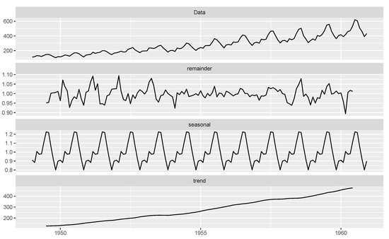
Figure 4.
Decomposition plot of the data.
After removing the seasonality and trend components, a time series plot of the data, with random components is produced, as shown in Figure 5.
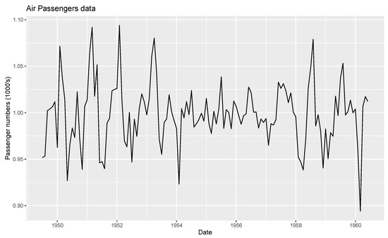
Figure 5.
Time series plot of random component.
The AR(1) model is fitted to the data with a correlation coefficient of = 0.4069 and an intercept = 0.9981. The ACF plot of residuals of the fitted AR(1) model is shown in Figure 6.
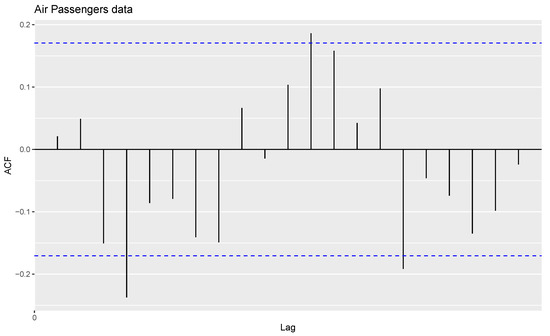
Figure 6.
Sample ACF of residuals of fitted AR(1) model.
Gaussian distribution with the parameters and is fitted to the data. And the acquired Kolmogorov-Smirnov (KS) statistic value is 0.083416, with corresponding p-value = 0.3173. This shows that Gaussian distribution is an appropriate fit for the data. The maximum likelihood estimates of the parameter are = 0.9982 and = 0.0332.
Using the maximum likelihood estimates, the estimate of extropy is . The extropy values are estimated using the proposed estimates given in Equations (6) and (4). The corresponding estimates are and . Thus, it becomes clear that the proposed estimate sits closer to the value and the estimate is far removed from the same value. As a result, the estimate is considered better than as a fit for the extropy data.
5.2. Application 2
For this application, the time series data ‘The Failure of Computer Patterns’ used in [22] is considered. These data comprise 257 observations, where the quantities relate to successive times-to-failures. The time series plot of the given data for this application is shown in Figure 7.
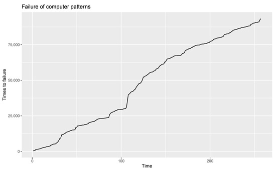
Figure 7.
Time series plot of the data “Failure of computer patterns”.
From an analysis of this time series plot, it becomes clear that data are non-stationary. Hence, the data are made stationary by calculating the difference. The time series plot of the stationary data is shown in Figure 8.
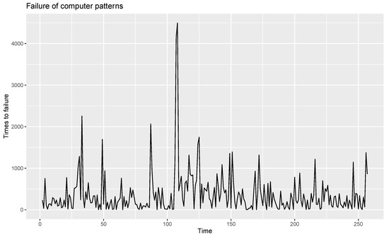
Figure 8.
Time series plot of stationary data.
For the given observations, eight outliers are present, and these are removed from the data. The time series plot, ACF and PACF of the remaining observations are shown in Figure 9, Figure 10 and Figure 11.
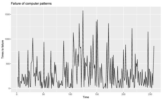
Figure 9.
Time series plot of computer failure data patterns without outliers.
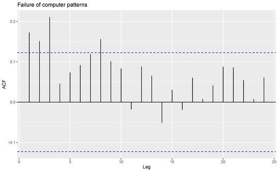
Figure 10.
ACF plot of computer failure data patterns without outliers.
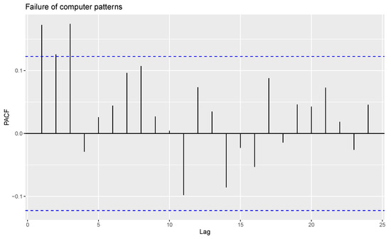
Figure 11.
PACF plot of computer failure data patterns without outliers.
The AR(1) model is fitted to the data and the correlation coefficient is obtained. Also, exponential distribution with the rate parameter is fitted to the data and we obtain KS = and p-value = 0.1121. Hence, it is apparent that the exponential distribution is a satisfactory fit to the data. The maximum likelihood estimate for the data is and the corresponding estimate for extropy is −0.0008186.
The estimates of extropy using kernel estimation are and . Thus, it becomes clear that the proposed estimate is closer to the estimate of extropy using the maximum likelihood estimation method, rather than the estimate of . Thus, is seen to be a better estimator than when fitting this data.
From the two applications discussed above, it is clear that the proposed estimator performed well in real-life scenario applications.
6. Conclusions and Future Works
This paper has explored the non-parametric estimators for extropy function using kernel type estimation, where observations under consideration are -mixing dependent. Certain asymptotic properties of the proposed estimator are investigated and proved. Furthermore, a simulation study has been conducted to compare the performance of the estimates, and the suitability of the estimator is shown using real-life data applications. It can be concluded that the proposed estimator is superior to .
Several generalizations of extropy function, such as weighted extropy and Tsallis extropy are proposed in the literature. Estimation of those generalizations based on dependent observations can be considered as one of the future works. In addition to the -mixing dependence condition one can develop inferential aspects of extropy and its various generalizations based on -mixing and -mixing dependence condition.
Author Contributions
Conceptualization, R.M., M.R.I. and H.B.; methodology, R.M., M.R.I. and A.K.; writing—original draft preparation, A.K.; review and editing, M.R.I., H. B. and N.Q.; validation, N.Q.; software, A.K. and N.Q.; visualization, A.K. and N.Q.; funding acquisition, N.Q. All authors have read and agreed to the published version of the manuscript.
Funding
This research was funded by Princess Nourah bint Abdulrahman University Researchers Supporting Project number (PNURSP2023R376), Princess Nourah bint Abdulrahman University, Riyadh, Saudi Arabia.
Institutional Review Board Statement
Not applicable.
Informed Consent Statement
Not applicable.
Data Availability Statement
The data presented in this study are available on request from the corresponding author.
Acknowledgments
The authors gratefully acknowledge Princess Nourah bint Abdulrahman University Researchers Supporting Project number (PNURSP2023R376), Princess Nourah bint Abdulrahman University, Riyadh, Saudi Arabia on the financial support for this project.
Conflicts of Interest
The authors declare no conflict of interest.
Appendix A
R-code to find by simulation for size n = 50
rm(list=ls())
library(MASS)
intt=function(x){
fn=h=rep()
for(i in 1:n)
{
h[i]=1/i^(0.5)
fn[i]=exp((-0.5/h[i]^2)*(x-X[i])^2)/(sqrt(2*pi)*h[i])
}
return((sum(fn)/n)^2)
}
n=50
for(s in 1:1000){
Jn[s]=(-1/2)*(integrate(Vectorize(intt),0,Inf)$value)
}
Jncap=mean(Jn)
References
- Shannon, C.E. A mathematical theory of communication. Bell Syst. Tech. J. 1948, 27, 379–423. [Google Scholar] [CrossRef]
- Cover, T.M.; Thomas, J.A. Elements of Information Theory, 2nd ed.; Wiley Series in Telecommunications and Signal Processing; John Wiley & Sons: Hoboken, NJ, USA, 2006. [Google Scholar]
- Frank, L.; Sanfilippo, G.; Agro, G. Extropy complementary dual of entropy. Stat. Sci. 2015, 30, 40–58. [Google Scholar]
- Jose, J.; Abdul Sathar, E.I. Extropy for past life based on classical records. J. Indian Soc. Probab. Stat. 2021, 22, 27–46. [Google Scholar] [CrossRef]
- Becerra, A.; de la Rosa, J.I.; Gonzàlez, E.; Pedroza, A.D.; Escalante, N.I. Training deep neural networks with non-uniform frame-level cost function for automatic speech recognition. Multimed. Tools Appl. 2018, 77, 27231–27267. [Google Scholar] [CrossRef]
- Martinas, K.; Frankowicz, M. Extropy-reformulation of the Entropy Principle. Period. Polytech. Chem. Eng. 2000, 44, 29–38. [Google Scholar]
- Qiu, G. The extropy of order statistics and record values. Stat. Probab. Lett. 2017, 120, 52–60. [Google Scholar] [CrossRef]
- Qiu, G.; Jia, K. Extropy estimators with applications in testing uniformity. J. Nonparametric Stat. 2018, 30, 182–196. [Google Scholar] [CrossRef]
- Rajesh, R.; Rajesh, G.; Sunoj, S. Kernel estimation of extropy function under length-biased sampling. Stat. Probab. Lett. 2022, 181, 109290. [Google Scholar] [CrossRef]
- Irshad, M.R.; Maya, R. Non-parametric log kernel estimation of extropy function. Chil. J. Stat. 2022, 13, 155–163. [Google Scholar]
- Rosenblatt, M. A central limit theorem and a strong mixing condition. Proc. Natl. Acad. Sci. USA 1956, 42, 43–47. [Google Scholar] [CrossRef] [PubMed]
- Irshad, M.R.; Maya, R. Non-parametric estimation of the past extropy under α-mixing dependence condition. Ric. Mat. 2022, 71, 723–734. [Google Scholar] [CrossRef]
- Maya, R.; Irshad, M.R. Kernel estimation of the residual extropy under α-mixing dependence condition. S. Afr. Stat. J. 2019, 53, 65–72. [Google Scholar] [CrossRef]
- Maya, R.; Irshad, M.R. Kernel estimation of Mathai-Haubold entropy and residual Mathai-Haubold entropy functions under α-mixing dependence condition. Am. J. Math. Manag. Sci. 2022, 41, 148–159. [Google Scholar] [CrossRef]
- Maya, R.; Irshad, M.R.; Archana, K. Recursive and non-recursive kernel estimation of negative cumulative residual extropy under α-mixing dependence condition. Ric. Mat. 2021, 55, 1–21. [Google Scholar] [CrossRef]
- Masry, E. Recursive probability density estimation for weakly dependent stationary processes. IEEE Trans. Inf. Theory 1986, 32, 254–267. [Google Scholar] [CrossRef]
- Härdle, W.K. Smoothing Techniques: With Implementation in S; Springer Science and Business Media: Berlin/Heidelberg, Germany, 1991. [Google Scholar]
- Hall, P.; Morton, S.C. On estimation of entropy. Ann. Inst. Stat. Math. 1993, 45, 69–88. [Google Scholar] [CrossRef]
- Wolverton, C.; Wagner, T. Asymptotically optimal discriminant functions for pattern classification. IEEE Trans. Inf. Theory 1969, 15, 258–265. [Google Scholar] [CrossRef]
- Wegman, E.J. Nonparametric probability density estimation: I. A summary of available methods. Technometrics 1972, 14, 533–546. [Google Scholar] [CrossRef]
- Box, G.E.; Jenkins, G.M.; Reinsel, G.C.; Ljung, G.M. Time Series Analysis: Forecasting and Control; John Wiley and Sons: Hoboken, NJ, USA, 2015. [Google Scholar]
- Lewis, P.A.W. A branching poisson process model for the analysis of computer failure patterns. J. R. Stat. Soc. Ser. (Methodol.) 1964, 26, 398–456. [Google Scholar] [CrossRef]
Disclaimer/Publisher’s Note: The statements, opinions and data contained in all publications are solely those of the individual author(s) and contributor(s) and not of MDPI and/or the editor(s). MDPI and/or the editor(s) disclaim responsibility for any injury to people or property resulting from any ideas, methods, instructions or products referred to in the content. |
© 2023 by the authors. Licensee MDPI, Basel, Switzerland. This article is an open access article distributed under the terms and conditions of the Creative Commons Attribution (CC BY) license (https://creativecommons.org/licenses/by/4.0/).