Approximate and Exact Solutions in the Sense of Conformable Derivatives of Quantum Mechanics Models Using a Novel Algorithm

Abstract

The entirety of the information regarding a subatomic particle is encoded in a wave function. Solving quantum mechanical models (QMMs) means finding the quantum mechanical wave function. Therefore, great attention has been paid to finding solutions for QMMs. In this study, a novel algorithm that combines the conformable Shehu transform and the Adomian decomposition method is presented that establishes approximate and exact solutions to QMMs in the sense of conformable derivatives with zero and nonzero trapping potentials. This solution algorithm is known as the conformable Shehu transform decomposition method (CSTDM). To evaluate the efficiency of this algorithm, the numerical results in terms of absolute and relative errors were compared with the reduced differential transform and the two-dimensional differential transform methods. The comparison showed excellent agreement with these methods, which means that the CSTDM is a suitable alternative tool to the methods based on the Caputo derivative for the solutions of time-fractional QMMs. The advantage of employing this approach is that, due to the use of the conformable Shehu transform, the pattern between the coefficients of the series solutions makes it simple to obtain the exact solution of both linear and nonlinear problems. Consequently, our approach is quick, accurate, and easy to implement. The convergence, uniqueness, and error analysis of the solution were examined using Banach’s fixed point theory.

1. Introduction

In some cases, fractional derivatives (FDs) are preferable to integer-order derivatives for modeling because they can simulate and examine complex structures with complicated nonlinear processes and higher-order behaviors. There are two main causes of this. First, rather than being limited to an integer order, we can choose any order for the FDs. Furthermore, when the mechanism has long-term memory, FDs are advantageously based on both past and present situations. In contrast to previous FDs, the conformable derivative (CD), which Khalil et al. developed, is a distinctive definition of a fractional derivative (FD) [1]. For a mapping $\vartheta \left(\varpi \right):[0,\infty ]\to \mathbb{R}$, the CD is given below [2]:

$$T_{\varpi }^{\sigma }\vartheta \left(\varpi \right)=\underset{ϵ\to 0}{lim}\frac{{\vartheta }^{\lceil \sigma \rceil -1}(\varpi +ϵ{\varpi }^{\lceil \sigma \rceil -\sigma })-{\vartheta }^{\lceil \sigma \rceil -1}\left(\varpi \right)}{ϵ},$$

(1)

where $m-1<\sigma \le m,\varpi >0$, $m\in \mathbb{N}$ and $\lceil \sigma \rceil$ is the lowest integer larger than or equivalent to $\sigma$. In a particular case, if $0<\sigma \le 1$, next, we obtain

$$T_{\varpi }^{\sigma }\vartheta \left(\varpi \right)=\underset{ϵ\to 0}{lim}\frac{\vartheta (\varpi +ϵ{\varpi }^{1-\sigma })-\vartheta \left(\varpi \right)}{ϵ},\varpi >0.$$

(2)

If $\vartheta \left(\varpi \right)$ is $\sigma$-differentiable in $(0,\mathcal{P})$, $\mathcal{P}>0$ and ${\displaystyle \underset{\varpi \to 0^{+}}{lim}{\vartheta }^{\sigma }\left(\varpi \right)}$ exists, then define ${\displaystyle {\vartheta }^{\left(\sigma \right)}\left(0\right)=\underset{\varpi \to 0^{+}}{lim}{\vartheta }^{\left(\sigma \right)}}$$\left(\varpi \right)$.

The advantages of the CD are explained as follows [3,4,5]:

i

In contrast to FDs, the CD satisfies all of the requirements and regulations for an ordinary derivative, such as the chain rule, the mean value theorem, the product, including Rolle’s theorem, and the quotient.

ii

The CD streamlines well-known integral transforms (ITs), such as the Laplace and Sumudu transforms, which are used to solve some fractional differential equations (FDEs).

iii

FDEs and systems can easily be solved analytically by the CD.

iv

As a result, new definitions, such as the class CD, Katugampola FD, M-CD, fuzzy generalized CD, and deformable CD, can be created.

v

The CD generates creative connections between the CD and earlier FDs in a variety of applications.

FDEs are frequently used for their logical support in the mathematical framework of physical problems, including technology, health care, monetary markets, and decision theory [6,7,8,9,10]. The solutions provided by FDEs are significant and useful. Therefore, great attention has been paid to the solutions offered by FDEs. Most nonlinear FDEs do not have exact solutions; therefore, approximate analytical methods have been established to find approximate solutions. Integral equations and DEs are all solved using ITs, which are one of the most useful mathematical techniques [11,12,13,14]. DEs can be transformed into the terms of an easy algebraic equation using the right integral transform (IT). ITs are linked to the work of P. S. Laplace in the 1780s and Joseph Fourier in 1822. Two well-known transformations, the Fourier transform and the Laplace transform (LT), were initially employed to address ordinary and partial DEs. After that, these ITs were applied to FDEs [15,16]. Researchers have devised a slew of new ITs to tackle a wide range of mathematical challenges in recent years. FDEs are solved by utilizing the fractional complex [17], the Elzaki [18], the Sumudu [19], the Aboodh [20], the travelling wave [21], and the ZZ [22] ITs. To handle FDEs, these transformations are utilized together with other numerical, analytical, or homotopy-based techniques. Many mathematicians have recently expressed interest in a new IT known as the shehu transform (ST).

The ST of $\vartheta \left(\varpi \right)$ is defined as follows:

$${\mathcal{S}}_{\sigma }\left[\vartheta \left(\varpi \right)\right]={\mathcal{G}}_{\sigma }(\mu ,\lambda )={\int }_0^{\infty }{exp}^{-\frac{\mu \varpi }{\lambda }}\vartheta \left(\varpi \right)d\varpi ,\mu >0,\lambda >0,$$

(3)

where $\mu$, $\lambda$ are variables.

These are the key strengths of the ST [23]:

i

The ST is easier to understand than the natural, LT, Sumudu, and Elzaki ITs.

ii

The ST becomes an LT when the variable $\lambda =1$ is employed and a Yang IT when the variable $\mu =1$ is used.

iii

The ST is a modification of the Sumudu and Laplace ITs.

iv

The ST can be used to obtain exact and approximate solutions to FDEs effectively.

v

The suggested IT can be regarded as a replacement tool for the natural, the Sumudu, the Laplace, and the Elzaki ITs for advanced study in physical science and engineering.

The Adomian decomposition method (ADM) is a semianalytical approach to solving both ordinary and partial DEs. George Adomian, the director of the University of Georgia’s Center for Applied Mathematics, developed the method from the 1970s through the 1990s. Particularly in the area of series solutions, the ADM has sparked a lot of attention in practical mathematics in recent years. The ADM entails breaking down each the unknown function $\vartheta (\zeta ,\varpi )$ of every equation into an infinite number of components described by the decomposition series ${\displaystyle \vartheta (\zeta ,\varpi )=\sum _{\upsilon =0}^{\infty }{\vartheta }_{\upsilon }(\zeta ,\varpi )}$, in this case, the components ${\vartheta }_{\upsilon }(\zeta ,\varpi )$, $\upsilon \ge 0$ must be calculated recursively.

Modern quantum mechanics was developed as a result of the inability of classical mechanics to explain a wide variety of physical phenomena, including microscopic processes such as black body radiation, atomic stability, and photoelectric reactions. This results from the discrete value quantization of all physical quantities in a bound system, which explains the phenomenon. In nuclear and atomic physics, as well as other areas of contemporary physics where the Schrödinger equation (SE) may be used to describe electron and nucleon activity, quantum mechanics can be utilized to explain how electrons behave in nucleons. Erwin Schrodinger, an Austrian physicist, created and published this equation in late 1925 [24].

Quantum mechanics is a probabilistic theory in the sense that the predictions it makes tell us, for instance, the probability of finding a particle somewhere in space. If there are no physical restrictions that would make it more likely for a particle to be at one location along the $\zeta –$axis than any other, and if we do not know anything about a particle’s prior history, the probability distribution must be $\vartheta (\zeta ,\varpi )=constant$. This is an example of a symmetry argument. Expressed more formally, it states that if the above conditions apply, then the probability distribution ought to be subject to the condition $\vartheta (\zeta +D,\varpi )=\vartheta (\zeta ,\varpi )$ for any constant value of D, and $\vartheta (\zeta ,\varpi )$= $constant$ is the only possible scenario in this case. In the language of physics, if there is nothing that gives the particle a higher probability of being at one point rather than another, then the probability is independent of position, and the system is invariant under displacement in the $\zeta$ direction. The above argument does not suffice for quantum mechanics, since, as we have learned, the fundamental quantity describing a particle is not the probability distribution, but the wave function $\vartheta (\zeta ,\varpi )$. Thus, the wave function, rather than the probability distribution, ought to be the quantity that is invariant under displacement, i.e., $\vartheta (\zeta +D,\varpi )=\vartheta (\zeta ,\varpi )$.

The Schrödinger equations (SEs) have been studied using a number of different approaches, including the Fourier-spectral approach [25], the residual power series [26], the fractional reduced differential transform [27], the homotopy perturbation [28], the differential transform method [29], the reduced differential transform method [30], and the two-dimensional differential transform method [31]. Each of these approaches has its own set of drawbacks and shortcomings, such as the fact that it takes computational resources and time to execute them. Additionally, there is a lot of literature on SE solutions that express FDs in Caputo terms. For this reason, we developed a novel algorithm that is the coupling approach of the conformable Shehu transform (CST) and ADM to acquire the approximate solution (App-S) and exact solution (Ex-S) of an SE. The numerical results obtained by the CSTDM were compared with those obtained by other methods, such as the reduced differential transform method (RDTM) [30] and the two-dimensional differential transform method (TDDTM) [31], in terms of absolute errors (Abs-E) and relative errors (Rel-E). The findings produced by the suggested method demonstrated great agreement with various methodologies, demonstrating its efficiency and reliability. For the solutions of time-fractional QMMs, the CSTDM is an appropriate substitute for tools based on Caputo derivatives. We also drew the conclusion that the CD is a good substitute for the Caputo derivative in the modeling of time-fractional QMMs.

The following is the nonlinear SE with respect to the time-fractional CD with nonzero trapping potential.

$$i{T}_{\varpi }^{\sigma }\vartheta (\zeta ,\varpi )+\delta {\vartheta }_{\zeta \zeta }(\zeta ,\varpi )+\Theta \left(\zeta \right)\vartheta (\zeta ,\varpi )+\Omega {\left|\vartheta (\zeta ,\varpi )\right|}^2\vartheta (\zeta ,\varpi )=0,$$

(4)

with the following initial condition (IC):

$$\vartheta (\zeta ,0)={\vartheta }_0\left(\zeta \right).$$

(5)

In this case, $\delta ,\Omega \in \mathbb{R}$, $0<\sigma \le 1$, $i^2=-1$; $T_{\varpi }^{\sigma }$ denotes a conformable FD of order $\sigma$; $\vartheta (\zeta ,\varpi )$ is a complex-valued function that requires determination, $\zeta \in \mathbb{R}$; $\varpi \ge 0$; $\Theta \left(\zeta \right)$ denotes the trapping potential; $\left|\vartheta \right(\zeta ,\varpi \left)\right|$ denotes the modulus of $\vartheta (\zeta ,\varpi )$. For $\sigma =1$, Equations (4) and (5) translate to a conventional nonlinear SE. When $\Omega =0$ is zero, the linear situation exists. We used the CSTDM with $\mathcal{S}\left(\zeta \right)=0$ and $\mathcal{S}\left(\zeta \right)\ne 0$ for both linear and nonlinear applications.

The paper’s structure is as follows. Section 2 illustrates the fundamental algorithms of the CSTDM in order to establish the solutions to the SEs. Additionally, this section discusses and demonstrates the convergence of the series solution as well as the uniqueness of the solution for the SE. In Section 3, the simplicity and effectiveness of the approach are illustrated by providing App-S and Ex-S to SEs. The numerical and graphic results obtained by using the CSTDM are evaluated in Section 4. Finally, we conclude the paper in Section 5.

2. Analysis of the CSTDM

The primary goal of this section is to provide a solution in the series form for the generalized SE using the CST and ADM. For the desired result, substitute $\vartheta (\zeta ,\varpi )={\vartheta }_1(\zeta ,\varpi )+i{\vartheta }_2(\zeta ,\varpi )$ into Equation (4) and, as a result, we obtain a system of equations.

$$\begin{array}{cc}\hfill T_{\varpi }^{\sigma }{\vartheta }_1(\zeta ,\varpi )=& -\delta D_{\zeta \zeta }{\vartheta }_2(\zeta ,\varpi )-\Theta \left(\zeta \right){\vartheta }_2(\zeta ,\varpi )-\Omega \left({\vartheta }_1^2(\zeta ,\varpi ){\vartheta }_2(\zeta ,\varpi )+{\vartheta }_2^3(\zeta ,\varpi )\right),\hfill \\ \hfill T_{\varpi }^{\sigma }{\vartheta }_2(\zeta ,\varpi )=& \delta D_{\zeta \zeta }{\vartheta }_1(\zeta ,\varpi )+\Theta \left(\zeta \right){\vartheta }_1(\zeta ,\varpi )+\Omega \left({\vartheta }_2^2(\zeta ,\varpi ){\vartheta }_1(\zeta ,\varpi )+{\vartheta }_1^3(\zeta ,\varpi )\right),\hfill \end{array}$$

(6)

with the following (IC):

$${\vartheta }_1(\zeta ,0)={\vartheta }_{1,0}(\zeta ,0),{\vartheta }_2(\zeta ,0)={\vartheta }_{2,0}(\zeta ,0),$$

(7)

where $\vartheta (\zeta ,0)={\vartheta }_{1,0}(\zeta ,0)+i{\vartheta }_{2,0}(\zeta ,0)$.

By applying ${\mathcal{S}}_{\sigma }$ to Equation (6),

$$\begin{array}{cc}\hfill {\mathcal{S}}_{\sigma }\left[T_{\varpi }^{\sigma }{\vartheta }_1(\zeta ,\varpi )\right]=& -{\mathcal{S}}_{\sigma }[\delta D_{\zeta \zeta }{\vartheta }_2(\zeta ,\varpi )+\Theta \left(\zeta \right){\vartheta }_2(\zeta ,\varpi )+\hfill \\ & \Omega \left({\vartheta }_1^2(\zeta ,\varpi ){\vartheta }_2(\zeta ,\varpi )+{\vartheta }_2^3(\zeta ,\varpi )\right)],\hfill \\ \hfill {\mathcal{S}}_{\sigma }\left[T_{\varpi }^{\sigma }{\vartheta }_2(\zeta ,\varpi )\right]=& {\mathcal{S}}_{\sigma }[\delta D_{\zeta \zeta }{\vartheta }_1(\zeta ,\varpi )+\Theta \left(\zeta \right){\vartheta }_1(\zeta ,\varpi )+\hfill \\ & \Omega \left({\vartheta }_2^2(\zeta ,\varpi ){\vartheta }_1(\zeta ,\varpi )+{\vartheta }_1^3(\zeta ,\varpi )\right)].\hfill \end{array}$$

(8)

By utilizing ${\mathcal{S}}_{\sigma }\left[T_{\varpi }^{\sigma }\vartheta (\zeta ,\varpi )\right]=\frac{\mu }{\lambda }{\mathcal{S}}_{\sigma }\left[\vartheta (\zeta ,\varpi )\right]-\vartheta (\zeta ,0)$, Equation (8) can be expressed as follows:

$$\begin{array}{cc}\hfill {\mathcal{S}}_{\sigma }\left[{\vartheta }_1(\zeta ,\varpi )\right]=& \frac{\lambda }{\mu }{\vartheta }_{1,0}(\zeta ,0)-\frac{\lambda }{\mu }{\mathcal{S}}_{\sigma }\left[\delta D_{\zeta \zeta }{\vartheta }_2(\zeta ,\varpi )\right]-\frac{\lambda }{\mu }{\mathcal{S}}_{\sigma }\left[\Theta \left(\zeta \right){\vartheta }_2(\zeta ,\varpi )\right]\hfill \\ & -\frac{\lambda }{\mu }{\mathcal{S}}_{\sigma }\left[\Omega \left({\vartheta }_1^2(\zeta ,\varpi ){\vartheta }_2(\zeta ,\varpi )+{\vartheta }_2^3(\zeta ,\varpi )\right)\right],\hfill \\ \hfill {\mathcal{S}}_{\sigma }\left[{\vartheta }_2(\zeta ,\varpi )\right]=& \frac{\lambda }{\mu }{\vartheta }_{2,0}(\zeta ,0)+\frac{\lambda }{\mu }{\mathcal{S}}_{\sigma }\left[\delta D_{\zeta \zeta }{\vartheta }_1(\zeta ,\varpi )\right]+\frac{\lambda }{\mu }{\mathcal{S}}_{\sigma }\left[\Theta \left(\zeta \right){\vartheta }_1(\zeta ,\varpi )\right]\hfill \\ & +\frac{\lambda }{\mu }{\mathcal{S}}_{\sigma }\left[\Omega \left({\vartheta }_2^2(\zeta ,\varpi ){\vartheta }_1(\zeta ,\varpi )+{\vartheta }_1^3(\zeta ,\varpi )\right)\right].\hfill \end{array}$$

(9)

By utilizing ${\mathcal{S}}_{\sigma }^{-1}$ in Equation (9), we have the following:

$$\begin{array}{cc}\hfill {\vartheta }_1(\zeta ,\varpi )=& {\mathcal{S}}_{\sigma }^{-1}\left[\frac{\lambda }{\mu }{\vartheta }_{1,0}(\zeta ,0)\right]-{\mathcal{S}}_{\sigma }^{-1}\left[\frac{\lambda }{\mu }{\mathcal{S}}_{\sigma }\left[\delta D_{\zeta \zeta }{\vartheta }_2(\zeta ,\varpi )\right]\right]-{\mathcal{S}}_{\sigma }^{-1}\left[\frac{\lambda }{\mu }{\mathcal{S}}_{\sigma }\left[\Theta \left(\zeta \right){\vartheta }_2(\zeta ,\varpi )\right]\right]\hfill \\ & -{\mathcal{S}}_{\sigma }^{-1}\left[\frac{\lambda }{\mu }{\mathcal{S}}_{\sigma }\left[\Omega \left({\vartheta }_1^2(\zeta ,\varpi ){\vartheta }_2(\zeta ,\varpi )+{\vartheta }_2^3(\zeta ,\varpi )\right)\right]\right],\hfill \\ \hfill {\vartheta }_2(\zeta ,\varpi )=& {\mathcal{S}}_{\sigma }^{-1}\left[\frac{\lambda }{\mu }{\vartheta }_{2,0}(\zeta ,0)\right]+{\mathcal{S}}_{\sigma }^{-1}\left[\frac{\lambda }{\mu }{\mathcal{S}}_{\sigma }\left[\delta D_{\zeta \zeta }{\vartheta }_1(\zeta ,\varpi )\right]\right]+{\mathcal{S}}_{\sigma }^{-1}\left[\frac{\lambda }{\mu }{\mathcal{S}}_{\sigma }\left[\Theta \left(\zeta \right){\vartheta }_1(\zeta ,\varpi )\right]\right]\hfill \\ & +{\mathcal{S}}_{\sigma }^{-1}\left[\frac{\lambda }{\mu }{\mathcal{S}}_{\sigma }\left[\Omega \left({\vartheta }_2^2(\zeta ,\varpi ){\vartheta }_1(\zeta ,\varpi )+{\vartheta }_1^3(\zeta ,\varpi )\right)\right)\right].\hfill \end{array}$$

(10)

So, according to the ADM, we can obtain solutions of ${\vartheta }_1(\zeta ,\varpi )$ and ${\vartheta }_2(\zeta ,\varpi )$ by using the following series:

$$\begin{array}{c}\hfill {\vartheta }_1(\zeta ,\varpi )=\sum _{\upsilon =0}^{\infty }{\vartheta }_{1,\upsilon }(\zeta ,\varpi ),\\ \hfill {\vartheta }_2(\zeta ,\varpi )=\sum _{\upsilon =0}^{\infty }{\vartheta }_{2,\upsilon }(\zeta ,\varpi ).\end{array}$$

(11)

The nonlinear terms ${\mathcal{N}}_1({\vartheta }_1,{\vartheta }_2)$ and ${\mathcal{N}}_2({\vartheta }_1,{\vartheta }_2)$ can be expressed as

$$\begin{array}{c}\hfill {\mathcal{N}}_1({\vartheta }_1,{\vartheta }_2)=\sum _{\upsilon =0}^{\infty }{\mathcal{Z}}_{1,\upsilon }({\vartheta }_1,{\vartheta }_2),\\ \hfill {\mathcal{N}}_2({\vartheta }_1,{\vartheta }_2)=\sum _{\upsilon =0}^{\infty }{\mathcal{Z}}_{2,\upsilon }({\vartheta }_1,{\vartheta }_2),\end{array}$$

(12)

where ${\mathcal{Z}}_{1,\upsilon }({\vartheta }_1,{\vartheta }_2)$ and ${\mathcal{Z}}_{2,\upsilon }({\vartheta }_1,{\vartheta }_2)$ represent the Adomian polynomials for the nonlinear term and are defined by the following formula:

$$\begin{array}{cc}\hfill {\mathcal{Z}}_{1,\upsilon }({\vartheta }_1,{\vartheta }_2)=& \frac{1}{\Gamma (\upsilon +1)}\frac{{\partial }^{\upsilon }}{\partial {\mathcal{L}}^{\upsilon }}{\left[{\mathcal{N}}_1\left(\sum _{\gamma =0}^{\upsilon }{\mathcal{L}}^{\gamma }{\vartheta }_{1,\gamma }(\zeta ,\varpi )\right)\right]}_{\mathcal{L}=0},\upsilon =0,1,2,\dots ,\hfill \\ \hfill {\mathcal{Z}}_{2,\upsilon }({\vartheta }_1,{\vartheta }_2)=& \frac{1}{\Gamma (\upsilon +1)}\frac{{\partial }^{\upsilon }}{\partial {\mathcal{L}}^{\upsilon }}{\left[{\mathcal{N}}_2\left(\sum _{\gamma =0}^{\upsilon }{\mathcal{L}}^{\gamma }{\vartheta }_{2,\gamma }(\zeta ,\varpi )\right)\right]}_{\mathcal{L}=0},\upsilon =0,1,2,\dots .\hfill \end{array}$$

(13)

We obtain the following results by putting Equations (11) and (12) into (10):

$$\begin{array}{cc}\hfill \sum _{\upsilon =0}^{\infty }{\vartheta }_{1,\upsilon }(\zeta ,\varpi )=& {\mathcal{S}}_{\sigma }^{-1}\left[\frac{\lambda }{\mu }{\vartheta }_{1,0}(\zeta ,0)\right]-{\mathcal{S}}_{\sigma }^{-1}\left[\frac{\lambda }{\mu }{\mathcal{S}}_{\sigma }\left[\delta D_{\zeta \zeta }\sum _{\upsilon =0}^{\infty }{\vartheta }_{2,\upsilon }(\zeta ,\varpi )\right]\right]-\hfill \\ & {\mathcal{S}}_{\sigma }^{-1}\left[\frac{w}{u}{\mathcal{S}}_{\sigma }\left[\Theta \left(\zeta \right)\sum _{\upsilon =0}^{\infty }{\vartheta }_{2,\upsilon }(\zeta ,\varpi )\right]\right]-{\mathcal{S}}_{\sigma }^{-1}[\frac{\lambda }{\mu }{\mathcal{S}}_{\sigma }\left[\Omega \sum _{\upsilon =0}^{\infty }{\mathcal{Z}}_{1,\upsilon }({\vartheta }_1,{\vartheta }_2)\right],\hfill \\ \hfill \sum _{\upsilon =0}^{\infty }{\vartheta }_{2,\upsilon }(\zeta ,\varpi )=& {\mathcal{S}}_{\sigma }^{-1}\left[\frac{\lambda }{\mu }{\vartheta }_{2,0}(\zeta ,0)\right]+{\mathcal{S}}_{\sigma }^{-1}\left[\frac{\lambda }{\mu }{\mathcal{S}}_{\sigma }\left[\delta D_{\zeta \zeta }\sum _{\upsilon =0}^{\infty }{\vartheta }_{1,\upsilon }(\zeta ,\varpi )\right]\right]+\hfill \\ & {\mathcal{S}}_{\sigma }^{-1}\left[\frac{\lambda }{\mu }{\mathcal{S}}_{\sigma }\left[\Theta \left(\zeta \right)\sum _{\upsilon =0}^{\infty }{\vartheta }_{1,\upsilon }(\zeta ,\varpi )\right]\right]+{\mathcal{S}}_{\sigma }^{-1}[\frac{\lambda }{\mu }{\mathcal{S}}_{\sigma }\left[\Omega \sum _{\upsilon =0}^{\infty }{\mathcal{Z}}_{2,\upsilon }({\vartheta }_1,{\vartheta }_2)\right].\hfill \end{array}$$

(14)

By comparing both ends of Equation (14), we obtain the following results:

$$\begin{array}{c}\hfill {\vartheta }_{1,0}(\zeta ,\varpi )={\mathcal{S}}_{\sigma }^{-1}\left[\frac{\lambda }{\mu }{\vartheta }_{1,0}(\zeta ,0)\right],\\ \hfill {\vartheta }_{2,0}(\zeta ,\varpi )={\mathcal{S}}_{\sigma }^{-1}\left[\frac{\lambda }{\mu }{\vartheta }_{2,0}(\zeta ,0)\right].\end{array}$$

(15)

In a similar manner, we attain the second term:

$$\begin{array}{cc}\hfill {\vartheta }_{1,1}(\zeta ,\varpi )=& -{\mathcal{S}}_{\sigma }^{-1}\left[\frac{\lambda }{\mu }{\mathcal{S}}_{\sigma }\left[\delta D_{\zeta \zeta }{\vartheta }_{2,0}(\zeta ,\varpi )\right]\right]-{\mathcal{S}}_{\sigma }^{-1}\left[\frac{\lambda }{\mu }{\mathcal{S}}_{\sigma }\left[\Theta \left(\zeta \right){\vartheta }_{2,0}(\zeta ,\varpi )\right]\right]-\hfill \\ & {\mathcal{S}}_{\sigma }^{-1}[\frac{\lambda }{\mu }{\mathcal{S}}_{\sigma }\left[\Omega {\mathcal{Z}}_{1,0}({\vartheta }_1,{\vartheta }_2)\right],\hfill \\ \hfill {\vartheta }_{2,1}(\zeta ,\varpi )=& {\mathcal{S}}_{\sigma }^{-1}\left[\frac{\lambda }{\mu }{\mathcal{S}}_{\sigma }\left[\delta D_{\zeta \zeta }{\vartheta }_{1,0}(\zeta ,\varpi )\right]\right]+{\mathcal{S}}_{\sigma }^{-1}\left[\frac{\lambda }{\mu }{\mathcal{S}}_{\sigma }\left[\Theta \left(\zeta \right){\vartheta }_{1,0}(\zeta ,\varpi )\right]\right]+\hfill \\ & {\mathcal{S}}_{\sigma }^{-1}[\frac{\lambda }{\mu }{\mathcal{S}}_{\sigma }\left[\Omega {\mathcal{Z}}_{2,0}({\vartheta }_1,{\vartheta }_2)\right].\hfill \end{array}$$

(16)

By repeating the same pattern, we determine the following third and fourth terms of the series solution of Equation (6):

$$\begin{array}{cc}\hfill {\vartheta }_{1,2}(\zeta ,\varpi )=& -{\mathcal{S}}_{\sigma }^{-1}\left[\frac{\lambda }{\mu }{\mathcal{S}}_{\zeta }\left[\delta D_{\zeta \zeta }{\vartheta }_{2,1}(\zeta ,\varpi )\right]\right]-{\mathcal{S}}_{\sigma }^{-1}\left[\frac{\lambda }{\mu }{\mathcal{S}}_{\sigma }\left[\Theta \left(\zeta \right){\vartheta }_{2,1}(\zeta ,\varpi )\right]\right]-\hfill \\ & {\mathcal{S}}_{\sigma }^{-1}[\frac{\lambda }{\mu }{\mathcal{S}}_{\sigma }\left[\Omega {\mathcal{Z}}_{1,1}({\vartheta }_1,{\vartheta }_2)\right],\hfill \\ \hfill {\vartheta }_{2,2}(\zeta ,\varpi )=& {\mathcal{S}}_{\sigma }^{-1}\left[\frac{\lambda }{\mu }{\mathcal{S}}_{\sigma }\left[\delta D_{\zeta \zeta }{\vartheta }_{1,1}(\zeta ,\varpi )\right]\right]+{\mathcal{S}}_{\sigma }^{-1}\left[\frac{\lambda }{\mu }{\mathcal{S}}_{\sigma }\left[\Theta \left(\zeta \right){\vartheta }_{1,1}(\zeta ,\varpi )\right]\right]+\hfill \\ & {\mathcal{S}}_{\sigma }^{-1}[\frac{\lambda }{\mu }{\mathcal{S}}_{\sigma }\left[\Omega {\mathcal{Z}}_{2,1}({\vartheta }_1,{\vartheta }_2)\right].\hfill \end{array}$$

(17)

$$\begin{array}{cc}\hfill {\vartheta }_{1,3}(\zeta ,\varpi )=& -{\mathcal{S}}_{\sigma }^{-1}\left[\frac{\lambda }{\mu }{\mathcal{S}}_{\sigma }\left[\delta D_{\zeta \zeta }{\vartheta }_{2,2}(\zeta ,\varpi )\right]\right]-{\mathcal{S}}_{\sigma }^{-1}\left[\frac{\lambda }{\mu }{\mathcal{S}}_{\sigma }\left[\Theta \left(\zeta \right){\vartheta }_{2,2}(\zeta ,\varpi )\right]\right]-\hfill \\ & {\mathcal{S}}_{\sigma }^{-1}[\frac{\lambda }{\mu }{\mathcal{S}}_{\sigma }\left[\Omega {\mathcal{Z}}_{1,2}({\vartheta }_1,{\vartheta }_2)\right],\hfill \\ \hfill {\vartheta }_{2,3}(\zeta ,\varpi )=& {\mathcal{S}}_{\sigma }^{-1}\left[\frac{\lambda }{\mu }{\mathcal{S}}_{\sigma }\left[\delta D_{\zeta \zeta }{\vartheta }_{1,2}(\zeta ,\varpi )\right]\right]+{\mathcal{S}}_{\sigma }^{-1}\left[\frac{\lambda }{\mu }{\mathcal{S}}_{\sigma }\left[\Theta \left(\zeta \right){\vartheta }_{1,2}(\zeta ,\varpi )\right]\right]+\hfill \\ & {\mathcal{S}}_{\sigma }^{-1}[\frac{\lambda }{\mu }{\mathcal{S}}_{\sigma }\left[\Omega {\mathcal{Z}}_{2,2}({\vartheta }_1,{\vartheta }_2)\right].\hfill \end{array}$$

(18)

By generalizing the terms of the series solutions for ${\vartheta }_1(\zeta ,\varpi )$ and ${\vartheta }_2(\zeta ,\varpi )$, we arrive at the following:

$$\begin{array}{cc}\hfill {\vartheta }_{1,\upsilon +1}(\zeta ,\varpi )=& -{\mathcal{S}}_{\sigma }^{-1}\left[\frac{\lambda }{\mu }{\mathcal{S}}_{\sigma }\left[\delta D_{\zeta \zeta }{\vartheta }_{2,\upsilon }(\zeta ,\varpi )\right]\right]-{\mathcal{S}}_{\sigma }^{-1}\left[\frac{\lambda }{\mu }{\mathcal{S}}_{\sigma }\left[\Theta \left(\zeta \right){\vartheta }_{2,\upsilon }(\zeta ,\varpi )\right]\right]-\hfill \\ & {\mathcal{S}}_{\sigma }^{-1}[\frac{w}{u}{\mathcal{S}}_{\sigma }\left[\Omega {\mathcal{Z}}_{1,\upsilon }({\vartheta }_1,{\vartheta }_2)\right],\hfill \\ \hfill {\vartheta }_{2,\upsilon +1}(\zeta ,\varpi )=& {\mathcal{S}}_{\sigma }^{-1}\left[\frac{\lambda }{\mu }{\mathcal{S}}_{\sigma }\left[\delta D_{\zeta \zeta }{\vartheta }_{1,\upsilon }(\zeta ,\varpi )\right]\right]+{\mathcal{S}}_{\sigma }^{-1}\left[\frac{\lambda }{\mu }{\mathcal{S}}_{\sigma }\left[\Theta \left(\zeta \right){\vartheta }_{1,\upsilon }(\zeta ,\varpi )\right]\right]+\hfill \\ & {\mathcal{S}}_{\sigma }^{-1}[\frac{\lambda }{\mu }{\mathcal{S}}_{\sigma }\left[\Omega {\mathcal{Z}}_{2,\upsilon }({\vartheta }_1,{\vartheta }_2)\right].\hfill \end{array}$$

(19)

Finally, we approximate the analytical solutions of ${\vartheta }_1(\zeta ,\varpi )$ and ${\vartheta }_2(\zeta ,\varpi )$ using the truncated series shown below.

$$\begin{array}{c}\hfill {\vartheta }_1(\zeta ,\varpi )=\underset{\gamma \to \infty }{lim}\sum _{\upsilon =0}^{\gamma }{\vartheta }_{1,\upsilon }(\zeta ,\varpi ),\\ \hfill {\vartheta }_2(\zeta ,\varpi )=\underset{\gamma \to \infty }{lim}\sum _{\upsilon =0}^{\gamma }{\vartheta }_{2,\upsilon }(\zeta ,\varpi ).\end{array}$$

(20)

The necessary condition that ensures there is only one solution is stated in the subsequent theorem.

Theorem 1.

When $0<{\rm Y}<1$ and ${\rm Y}=({\ell }_1+{\ell }_2)\left(\frac{{\varpi }^{\sigma }}{\sigma }\right)$, Equation (6) has a unique solution.

Proof. 

We establish a function $\mathcal{G}:\mho ⟶\mho$ with the following assumption that $\mho =\left(\mathcal{Y}\right[0,\mathcal{W}],\Vert .\Vert )$ is the Banach space of all continuous functions.

$${\vartheta }_{1,\upsilon +1}(\zeta ,\frac{{\varpi }^{\sigma }}{\sigma })={\vartheta }_1(\zeta ,0)+{\mathcal{S}}_{\sigma }^{-1}\left[\frac{\lambda }{\mu }{\mathcal{S}}_{\sigma }\left[\mathcal{Q}\left({\vartheta }_{1,\upsilon }(\zeta ,\frac{{\varpi }^{\sigma }}{\sigma }\right)+\mathcal{X}\left({\vartheta }_{1,\upsilon }(\zeta ,\frac{{\varpi }^{\sigma }}{\sigma })\right)\right]\right],$$

(21)

with $\upsilon =0,1,2,\dots$ and $\mathcal{Q}\left({\vartheta }_1(\zeta ,\frac{{\varpi }^{\sigma }}{\sigma })\right)=-\delta D_{\zeta \zeta }{\vartheta }_2(\zeta ,\frac{{\varpi }^{\sigma }}{\sigma })-\mathcal{S}\left(\zeta \right){\vartheta }_2(\zeta ,\frac{{\varpi }^{\sigma }}{\sigma })$. Now, assume that $\mathcal{Q}$ and $\mathcal{X}$ are also Lipschitzian with $\Vert \mathcal{Q}{\vartheta }_1-\mathcal{Q}{\widehat{\vartheta }}_1\Vert <{\ell }_1\Vert {\vartheta }_1-{\widehat{\vartheta }}_1\Vert$ and $\Vert \mathcal{X}{\vartheta }_1-\mathcal{X}{\widehat{\vartheta }}_1\Vert <{\ell }_2\Vert {\vartheta }_1-{\widehat{\vartheta }}_1\Vert$, where ${\ell }_1$ and ${\ell }_2$ are Lipschitz constants and ${\vartheta }_1$ and ${\widehat{\vartheta }}_1$ are distinct functions.

$$\begin{array}{cc}\hfill \Vert \mathcal{G}{\vartheta }_1-\mathcal{G}{\widehat{\vartheta }}_{1,\upsilon }\Vert =& \mid {\mathcal{S}}_{\sigma }^{-1}\left[\frac{\lambda }{\mu }{\mathcal{S}}_{\sigma }\left[\mathcal{Q}\left({\vartheta }_{1,\upsilon }(\zeta ,\frac{{\varpi }^{\sigma }}{\sigma }\right)+\mathcal{X}\left({\vartheta }_{1,\upsilon }(\zeta ,\frac{{\varpi }^{\sigma }}{\sigma })\right)\right]\right]-\hfill \\ & {\mathcal{S}}_{\sigma }^{-1}\left[\frac{\lambda }{\mu }{\mathcal{S}}_{\sigma }\left[\mathcal{Q}\left({\widehat{\vartheta }}_{1,\upsilon }(\zeta ,\frac{{\varpi }^{\sigma }}{\sigma }\right)+\mathcal{X}\left({\widehat{\vartheta }}_{1,\upsilon }(\zeta ,\frac{{\varpi }^{\sigma }}{\sigma })\right)\right]\right]\mid \hfill \\ \hfill \le & \underset{\varpi \in [0,\mathcal{W}]}{max}\mid {\mathcal{S}}_{\sigma }^{-1}\left[\frac{\lambda }{\mu }{\mathcal{S}}_{\sigma }\right[\mathcal{Q}\left({\vartheta }_{1,\upsilon }(\zeta ,\frac{{\varpi }^{\sigma }}{\sigma })\right)-\mathcal{Q}\left({\widehat{\vartheta }}_{1,\upsilon }(\zeta ,\frac{{\varpi }^{\sigma }}{\sigma })\right]+\hfill \\ & {\mathcal{S}}_{\sigma }^{-1}\left[\frac{\lambda }{\mu }{\mathcal{S}}_{\sigma }\right[\mathcal{X}\left({\vartheta }_{1,\upsilon }(\zeta ,\frac{{\varpi }^{\sigma }}{\sigma })\right)-\mathcal{X}\left({\widehat{\vartheta }}_{1,\upsilon }(\zeta ,\frac{{\varpi }^{\sigma }}{\sigma })\right]\mid \hfill \\ \hfill \le & \underset{\varpi \in [0,\mathcal{W}]}{max}({\ell }_1{\mathcal{S}}_{\sigma }^{-1}\left[\frac{\lambda }{\mu }{\mathcal{S}}_{\sigma }\left[\mid {\vartheta }_{1,\upsilon }(\zeta ,\frac{{\varpi }^{\sigma }}{\sigma })-{\widehat{\vartheta }}_{1,\upsilon }(\zeta ,\frac{{\varpi }^{\sigma }}{\sigma })\mid \right]\right]+\hfill \\ & {\ell }_2{\mathcal{S}}_{\sigma }^{-1}\left[\frac{\lambda }{\mu }{\mathcal{S}}_{\sigma }\left[\mid {\vartheta }_{1,\upsilon }(\zeta ,\frac{{\varpi }^{\sigma }}{\sigma })-{\widehat{\vartheta }}_{1,\upsilon }(\zeta ,\frac{{\varpi }^{\sigma }}{\sigma })\mid \right]\right])\hfill \\ \hfill \le & \underset{\varpi \in [0,\mathcal{W}]}{max}({\ell }_1+{\ell }_2)\left({\mathcal{S}}_{\sigma }^{-1}\left[\frac{\lambda }{\mu }{\mathcal{S}}_{\sigma }\left[\mid {\vartheta }_{1,\upsilon }(\zeta ,\frac{{\varpi }^{\sigma }}{\sigma })-{\widehat{\vartheta }}_{1,\upsilon }(\zeta ,\frac{{\varpi }^{\sigma }}{\sigma })\mid \right]\right]\right)\hfill \\ \hfill \le & \underset{\varpi \in [0,\mathcal{W}]}{max}({\ell }_1+{\ell }_2)\left({\mathcal{S}}_{\sigma }^{-1}\left[\frac{\lambda }{\mu }{\mathcal{S}}_{\sigma }\left[\Vert {\vartheta }_{1,\upsilon }(\zeta ,\frac{{\varpi }^{\sigma }}{\sigma })-{\widehat{\vartheta }}_{1,\upsilon }(\zeta ,\frac{{\varpi }^{\sigma }}{\sigma })\Vert \right]\right]\right)\hfill \\ \hfill =& ({\ell }_1+{\ell }_2)\left(\frac{{\varpi }^{\sigma }}{\sigma }\right)\Vert {\vartheta }_{1,\upsilon }(\zeta ,\frac{{\varpi }^{\sigma }}{\sigma })-{\widehat{\vartheta }}_{1,\upsilon }(\zeta ,\frac{{\varpi }^{\sigma }}{\sigma })\Vert .\hfill \end{array}$$

When $0<{\rm Y}<1$, the function $\mathcal{G}$ is a contraction. By the Banach fixed point theorem for contraction, Equation (6) has a unique solution. □

The following theorem illustrates and establishes the series solution convergence criterion.

Theorem 2.

The solution of Equation (6) is convergent.

Proof. 

Let ${\displaystyle {\mathcal{D}}_{\gamma }=\sum _{\upsilon =0}^{\gamma }{\vartheta }_{1,\upsilon }(\zeta ,\frac{{\varpi }^{\sigma }}{\sigma })}$ be the $\gamma th$ partial sum. Utilizing a new formulation of the Adomian polynomial, we have

$${\displaystyle \mathcal{X}\left({\mathcal{D}}_{\gamma }\right)=\sum _{\upsilon =0}^{\gamma }{\hat{\mathcal{A}}}_{1,\upsilon }.}$$

Now,

$$\begin{array}{cc}\hfill \Vert {\mathcal{D}}_{\gamma }-{\mathcal{D}}_{\beta }\Vert =& \underset{\varpi \in [0,\mathcal{W}]}{max}\mid {\mathcal{D}}_{\gamma }-{\mathcal{D}}_{\beta }\mid \hfill \\ \hfill =& \underset{\varpi \in [0,\mathcal{W}]}{max}\mid \sum _{\upsilon =\alpha +1}^{\gamma }{\widehat{\vartheta }}_{1,\upsilon }(\zeta ,\varpi )\mid \hfill \\ \hfill \le & \underset{\varpi \in [0,\mathcal{W}]}{max}\mid {\mathcal{S}}_{\sigma }^{-1}\left[\frac{\lambda }{\mu }{\mathcal{S}}_{\sigma }\left[\mathcal{Q}\left(\sum _{\upsilon =\alpha +1}^{\gamma }{\vartheta }_{1,\upsilon }\right)\right]\right]+{\mathcal{S}}_{\sigma }^{-1}\left[\frac{\lambda }{\mu }{\mathcal{S}}_{\sigma }\left[\mathcal{X}\left(\sum _{\upsilon =\alpha +1}^{\gamma }{\mathcal{A}}_{1,\upsilon }\right)\right]\right]\mid \hfill \\ \hfill \le & \underset{\varpi \in [0,\mathcal{W}]}{max}\mid [{\mathcal{S}}_{\sigma }^{-1}\frac{\lambda }{\mu }\left[{\mathcal{S}}_{\sigma }\left[\sum _{\upsilon =\alpha +1}^{\gamma }\mathcal{Q}\left({\mathcal{D}}_{\gamma -1}\right)-\mathcal{Q}\left({\mathcal{D}}_{\alpha -1}\right)\right]\right]+\hfill \\ & {\mathcal{S}}_{\sigma }^{-1}\left[\frac{\lambda }{\mu }{\mathcal{S}}_{\sigma }\left[\sum _{\upsilon =\alpha +1}^{\gamma }\mathcal{X}\left({\mathcal{D}}_{\gamma -1}\right)-\mathcal{X}\left({\mathcal{D}}_{\alpha -1}\right)\right]\right]\mid \hfill \\ \hfill \le & \underset{\varpi \in [0,\mathcal{W}]}{max}\mid [{\mathcal{S}}_{\sigma }^{-1}\frac{\lambda }{\mu }\left[{\mathcal{S}}_{\sigma }\left[\mathcal{Q}\left({\mathcal{D}}_{\gamma -1}\right)-\mathcal{Q}\left({\mathcal{D}}_{\alpha -1}\right)\right]\right]+\hfill \\ & {\mathcal{S}}_{\sigma }^{-1}\left[\frac{\lambda }{\mu }{\mathcal{S}}_{\sigma }\left[\mathcal{X}\left({\mathcal{D}}_{\gamma -1}\right)-\mathcal{X}\left({\mathcal{D}}_{\alpha -1}\right)\right]\right]\mid \hfill \\ \hfill \le & \underset{\varpi \in [0,\mathcal{W}]}{max}({\ell }_1+{\ell }_2)\left({\mathcal{S}}_{\sigma }^{-1}\left[\frac{\lambda }{\mu }{\mathcal{S}}_{\sigma }\left[\Vert {\mathcal{D}}_{\gamma -1}-{\mathcal{D}}_{\alpha -1}\Vert \right]\right]\right)\hfill \\ \hfill =& ({\ell }_1+{\ell }_2)\left(\frac{{\varpi }^{\sigma }}{\sigma }\right)\Vert {\mathcal{D}}_{\gamma -1}-{\mathcal{D}}_{r-1}\Vert \hfill \\ \hfill =& {\rm Y}\Vert {\mathcal{D}}_{\gamma -1}-{\mathcal{D}}_{r-1}\Vert .\hfill \end{array}$$

Let $\gamma =\alpha +1$, we have $\Vert {\mathcal{D}}_{\alpha +1}-{\mathcal{D}}_{\alpha }\Vert \le {{\rm Y}}^{\alpha }\Vert {\mathcal{D}}_1-{\mathcal{D}}_0\Vert$. By using the triangle inequality we have $\Vert {\mathcal{D}}_{\alpha +1}-{\mathcal{D}}_{\alpha }\Vert \le ({{\rm Y}}^{\alpha -1}-1)\Vert {\vartheta }_{1,1}(\zeta ,\frac{{\varpi }^{\sigma }}{\sigma })\Vert$, but since $0<{\rm Y}<1$, $0<1-{\rm Y}<1$, this implies that $\Vert {\mathcal{D}}_{\alpha +1}-{\mathcal{D}}_{\alpha }\Vert \le \frac{{{\rm Y}}^{\alpha }}{1-{\rm Y}}\underset{\varpi \in [0,\mathcal{W}]}{max}\Vert {\mathcal{D}}_1\Vert .\Vert {\vartheta }_{1,1}(\zeta ,\varpi )\Vert$ is finite, thus as $\alpha \to \infty$, $\Vert {\mathcal{D}}_{\alpha +1}-{\mathcal{D}}_{\alpha }\Vert \to 0$, hence $\left\{{\mathcal{D}}_{\alpha }\right\}$ is a Cauchy sequence in the Banach space ℧, thus the solution ${\displaystyle \underset{\gamma \to \infty }{lim}\sum _{\upsilon =0}^{\gamma }{\vartheta }_{1,\upsilon }(\zeta ,\frac{{\varpi }^{\sigma }}{\sigma })}$ is convergent. □

The maximum absolute truncation error (MATE) of the series solution ${\displaystyle \underset{\gamma \to \infty }{lim}\sum _{\upsilon =0}^{\gamma }{\vartheta }_{1,\upsilon }(\zeta ,\frac{{\varpi }^{\sigma }}{\sigma })}$ is addressed in the next theorem.

Theorem 3.

The MATE of Equation (20) to Equation (6) can be calculated as follows:

$${\displaystyle \Vert {\vartheta }_1(\zeta ,\frac{{\varpi }^{\sigma }}{\sigma })-\sum _{\upsilon =1}^{\alpha }{\vartheta }_{1,\upsilon }(\zeta ,\frac{{\varpi }^{\sigma }}{\sigma })\Vert \le \frac{{{\rm Y}}^{\alpha }}{1-{\rm Y}}\underset{\varpi \in [0,\mathcal{W}]}{max}\Vert {\vartheta }_{1,1}(\zeta ,\frac{{\varpi }^{\sigma }}{\sigma })\Vert .}$$

Proof. 

From Theorem 2, we have $\Vert {\mathcal{D}}_{\gamma }-{\mathcal{D}}_{\beta }\Vert \le \frac{{{\rm Y}}^{\beta }}{1-{\rm Y}}\underset{\varpi \in [0,\mathcal{W}]}{max}\Vert {\vartheta }_{1,1}(\zeta ,\frac{{\varpi }^{\sigma }}{\sigma })\Vert$, as $n\to \infty$, ${\mathcal{D}}_{\gamma }\to {\vartheta }_1(\zeta ,\frac{{\varpi }^{\sigma }}{\sigma })$. Thus, we have

$$\begin{array}{cc}\hfill \Vert {\vartheta }_1(\zeta ,\frac{{\varpi }^{\sigma }}{\sigma })-\sum _{\upsilon =1}^{\alpha }{\vartheta }_{1,\upsilon }(\zeta ,\frac{{\varpi }^{\sigma }}{\sigma })\Vert =& \underset{\varpi \in [0,\mathcal{W}]}{max}\mid {\vartheta }_1(\zeta ,\frac{{\varpi }^{\sigma }}{\sigma })-\sum _{\upsilon =1}^{\alpha }{\vartheta }_{1,\upsilon }(\zeta ,\frac{{\varpi }^{\sigma }}{\sigma })\mid \hfill \\ \hfill \le & \frac{{{\rm Y}}^{\beta }}{1-{\rm Y}}\underset{\varpi \in [0,\mathcal{W}]}{max}\Vert {\vartheta }_{1,1}(\zeta ,\frac{{\varpi }^{\sigma }}{\sigma })\Vert ,\hfill \end{array}$$

which confirms the theorem. □

The appropriateness of the CSTDM is determined in the following section.

3. Applications

In this section, three QMMs are solved to demonstrate the usefulness and applicability of the novel algorithm.

Problem 1.

In our first illustration, we take the linear SE provided below.

$$i{T}_{\varpi }^{\sigma }\vartheta (\zeta ,\varpi )-D_{\zeta \zeta }\vartheta (\zeta ,\varpi )=0,\varpi \ge 0,0<\sigma \le 1,$$

(22)

with the following IC:

$$\vartheta (\zeta ,0)=1+cosh\left(2\zeta \right),\zeta \in \mathbb{R}.$$

(23)

To achieve the desired outcome, use $\vartheta (\zeta ,\varpi )={\vartheta }_1(\zeta ,\varpi )+i{\vartheta }_2(\zeta ,\varpi )$ in Equation (22) and $\vartheta (\zeta ,0)={\vartheta }_{1,0}\left(\zeta \right)+i{\vartheta }_{2,0}\left(\zeta \right)$ in Equation (23), and, as a result, we obtain the coupled system shown below:

$$\begin{array}{cc}\hfill T_{\varpi }^{\sigma }{\vartheta }_1(\zeta ,\varpi )=& D_{\zeta \zeta }{\vartheta }_2(\zeta ,\varpi ),\hfill \\ \hfill T_{\varpi }^{\sigma }{\vartheta }_2(\zeta ,\varpi )=& -D_{\zeta \zeta }{\vartheta }_1(\zeta ,\varpi ),\hfill \end{array}$$

(24)

subject to the IC

$$\begin{array}{cc}\hfill {\vartheta }_{1,0}(\zeta ,0)=& 1+cosh\left(2\zeta \right),\hfill \\ \hfill {\vartheta }_{2,0}(\zeta ,0)=& 0.\hfill \end{array}$$

(25)

By following the steps that were established in Section 3, we obtain the following result:

$$\begin{array}{c}\hfill {\mathcal{S}}_{\sigma }\left[{\vartheta }_1(\zeta ,\varpi )\right]=\frac{\lambda }{\mu }{\vartheta }_{1,0}(\zeta ,0)+\frac{\lambda }{\mu }{\mathcal{S}}_{\sigma }\left[D_{\zeta \zeta }{\vartheta }_2(\zeta ,\varpi )\right],\\ \hfill {\mathcal{S}}_{\sigma }\left[{\vartheta }_2(\zeta ,\varpi )\right]=\frac{\lambda }{\mu }{\vartheta }_{2,0}(\zeta ,0)-\frac{\lambda }{\mu }{\mathcal{S}}_{\sigma }\left[D_{\zeta \zeta }{\vartheta }_1(\zeta ,\varpi )\right].\end{array}$$

(26)

Utilizing ${\mathcal{S}}_{\sigma }^{-1}$ in Equation (26), we obtain the following:

$$\begin{array}{cc}\hfill {\vartheta }_1(\zeta ,\varpi )=& {\mathcal{S}}_{\sigma }^{-1}\left[\frac{\lambda }{\mu }{\vartheta }_{1,0}(\zeta ,0)\right]+{\mathcal{S}}_{\sigma }^{-1}\left[\frac{\lambda }{\mu }{\mathcal{S}}_{\sigma }\left[D_{\zeta \zeta }{\vartheta }_2(\zeta ,\varpi )\right]\right],\hfill \\ \hfill {\vartheta }_2(\zeta ,\varpi )=& {\mathcal{S}}_{\sigma }^{-1}\left[\frac{\lambda }{\mu }{\vartheta }_{2,0}(\zeta ,0)\right]-{\mathcal{S}}_{\sigma }^{-1}\left[\frac{\lambda }{\mu }{\mathcal{S}}_{\sigma }\left[D_{\zeta \zeta }{\vartheta }_1(\zeta ,\varpi )\right]\right].\hfill \end{array}$$

(27)

Using the approach outlined in Section 3, we derive the following result from Equation (27):

$$\begin{array}{cc}\hfill \sum _{\upsilon =0}^{\infty }{\vartheta }_{1,\upsilon }(\zeta ,\varpi )=& {\mathcal{S}}_{\sigma }^{-1}\left[\frac{\lambda }{\mu }{\vartheta }_{1,0}(\zeta ,0)\right]+{\mathcal{S}}_{\sigma }^{-1}\left[\frac{\lambda }{\mu }{\mathcal{S}}_{\sigma }\left[D_{\zeta \zeta }\sum _{\upsilon =0}^{\infty }{\vartheta }_{2,\upsilon }(\zeta ,\varpi )\right]\right],\hfill \\ \hfill \sum _{\upsilon =0}^{\infty }{\vartheta }_{2,\upsilon }(\zeta ,\varpi )=& {\mathcal{S}}_{\sigma }^{-1}\left[\frac{\lambda }{\mu }{\vartheta }_{2,0}(\zeta ,0)\right]-{\mathcal{S}}_{\sigma }^{-1}\left[\frac{\lambda }{\mu }{\mathcal{S}}_{\sigma }\left[D_{\zeta \zeta }\sum _{\upsilon =0}^{\infty }{\vartheta }_{1,\upsilon }(\zeta ,\varpi )\right]\right].\hfill \end{array}$$

(28)

We obtain the following first term of the series solution:

$$\begin{array}{cc}\hfill {\vartheta }_{1,0}(\zeta ,\varpi )=& 1+cosh\left(2\zeta \right),\hfill \\ \hfill {\vartheta }_{2,0}(\zeta ,\varpi )=& 0.\hfill \end{array}$$

(29)

We obtain the following second terms from Equation (28):

$$\begin{array}{cc}\hfill {\vartheta }_{1,1}(\zeta ,\varpi )=& 0,\hfill \\ \hfill {\vartheta }_{2,1}(\zeta ,\varpi )=& -\frac{4}{\Gamma \left(2\right)}cosh\left(2\zeta \right)\frac{{\varpi }^{\sigma }}{\sigma }.\hfill \end{array}$$

(30)

By repeating the same process, we obtain the third term from Equation (28):

$$\begin{array}{cc}\hfill {\vartheta }_{1,2}(\zeta ,\varpi )=& -\frac{8}{\Gamma \left(3\right)}cosh\left(2\zeta \right)\frac{{\varpi }^{2\sigma }}{{\sigma }^2},\hfill \\ \hfill {\vartheta }_{2,2}(\zeta ,\varpi )=& 0.\hfill \end{array}$$

(31)

The fourth, fifth, and sixth terms of the series solution for Equation (24) were also determined in the same manner:

$$\begin{array}{cc}\hfill {\vartheta }_{1,3}(\zeta ,\varpi )=& 0,\hfill \\ \hfill {\vartheta }_{2,3}(\zeta ,\varpi )=& \frac{64}{\Gamma \left(4\right)}cosh\left(2\zeta \right)\frac{{\varpi }^{3\sigma }}{{\sigma }^3}.\hfill \end{array}$$

(32)

$$\begin{array}{cc}\hfill {\vartheta }_{1,4}(\zeta ,\varpi )=& \frac{256}{\Gamma \left(5\right)}cosh\left(2\zeta \right)\frac{{\varpi }^{4\sigma }}{{\sigma }^4},\hfill \\ \hfill {\vartheta }_{2,4}(\zeta ,\varpi )=& 0.\hfill \end{array}$$

(33)

$$\begin{array}{cc}\hfill {\vartheta }_{1,5}(\zeta ,\varpi )=& 0,\hfill \\ \hfill {\vartheta }_{2,5}(\zeta ,\varpi )=& -\frac{1024}{\Gamma \left(6\right)}cosh\left(2\zeta \right)\frac{{\varpi }^{5\sigma }}{{\sigma }^5}.\hfill \end{array}$$

(34)

The series solution to Equation (22) is given below:

$$\vartheta (\zeta ,\varpi )=1+cosh\left(2\zeta \right)\left(\sum _{\upsilon =0}^{\infty }\frac{{(-1)}^{\upsilon }}{\Gamma (2\upsilon +1)}{\left(\frac{4{\varpi }^{\sigma }}{\sigma }\right)}^{2\upsilon }-i\sum _{\upsilon =0}^{\infty }\frac{{(-1)}^{\upsilon }}{\Gamma (2\upsilon +2)}{\left(\frac{4{\varpi }^{\sigma }}{\sigma }\right)}^{2\upsilon +1}\right).$$

(35)

The Ex-S obtained by using the CSTDM at $\sigma =1.0$ is $1+cosh\left(2\zeta \right){exp}^{-4i\varpi }$.

Problem 2.

Consider the following nonlinear SE:

$$i{T}_{\varpi }^{\sigma }\vartheta (\zeta ,\varpi )+{\vartheta }_{\zeta \zeta }(\zeta ,\varpi )+2{\left|\vartheta (\zeta ,\varpi )\right|}^2\vartheta (\zeta ,\varpi )=0,$$

(36)

with the IC

$$\vartheta (\zeta ,0)={exp}^{i\zeta }, \zeta \in \mathbb{R}.$$

(37)

To obtain the required result, use $\vartheta (\zeta ,\varpi )={\vartheta }_1(\zeta ,\varpi )+i{\vartheta }_2(\zeta ,\varpi )$ and $\vartheta (\zeta ,0)={\vartheta }_{1,0}\left(\zeta \right)+i{\vartheta }_{2,0}\left(\zeta \right)$ in Equation (36) and Equation (37), respectively. As a result, we have the coupled system shown below:

$$\begin{array}{cc}\hfill T_{\varpi }^{\sigma }{\vartheta }_1(\zeta ,\varpi )& =-D_{\zeta \zeta }{\vartheta }_2(\zeta ,\varpi )-2\left({\vartheta }_1^2(\zeta ,\varpi ){\vartheta }_2(\zeta ,\varpi )+{\vartheta }_2^3(\zeta ,\varpi )\right),\hfill \\ \hfill T_{\tau }^{\sigma }{\vartheta }_2(\zeta ,\varpi )& =D_{\zeta \zeta }{\vartheta }_1(\zeta ,\varpi )+2\left({\vartheta }_2^2(\zeta ,\varpi ){\vartheta }_1(\zeta ,\varpi )+{\vartheta }_1^3(\zeta ,\varpi )\right),\hfill \end{array}$$

(38)

with the IC

$$\begin{array}{c}\hfill {\vartheta }_1(\zeta ,0)=cos\left(\zeta \right),\\ \hfill {\vartheta }_2(\zeta ,0)=sin\left(\zeta \right).\end{array}$$

(39)

Using the procedures outlined in Section 3, we obtain the following outcome:

$$\begin{array}{cc}\hfill {\mathcal{S}}_{\sigma }\left[{\vartheta }_1(\zeta ,\varpi )\right]=& \frac{\lambda }{\mu }{\vartheta }_{1,0}(\zeta ,0)-\frac{\lambda }{\mu }{\mathcal{S}}_{\sigma }\left[D_{\zeta \zeta }{\vartheta }_2(\zeta ,\varpi )\right]\hfill \\ & -\frac{\lambda }{\mu }{\mathcal{S}}_{\sigma }\left[2\left({\vartheta }_1^2(\zeta ,\varpi ){\vartheta }_2(\zeta ,\varpi )+{\vartheta }_2^3(\zeta ,\varpi )\right)\right],\hfill \\ \hfill {\mathcal{S}}_{\sigma }\left[{\vartheta }_2(\zeta ,\varpi )\right]=& \frac{\lambda }{\mu }{\vartheta }_{2,0}(\zeta ,0)+\frac{\lambda }{\mu }{\mathcal{S}}_{\sigma }\left[D_{\zeta \zeta }{\vartheta }_1(\zeta ,\varpi )\right]\hfill \\ & +\frac{\lambda }{\mu }{\mathcal{S}}_{\sigma }\left[2\left({\vartheta }_2^2(\zeta ,\varpi ){\vartheta }_1(\zeta ,\varpi )+{\vartheta }_1^3(\zeta ,\varpi )\right)\right].\hfill \end{array}$$

(40)

Using ${\mathcal{S}}_{\sigma }^{-1}$ in Equation (40), we have the following:

$$\begin{array}{cc}\hfill {\vartheta }_1(\upsilon ,\tau )=& {\mathcal{S}}_{\sigma }^{-1}\left[\frac{\lambda }{\mu }{\vartheta }_{1,0}(\zeta ,0)\right]-{\mathcal{S}}_{\sigma }^{-1}\left[\frac{\lambda }{\mu }{\mathcal{S}}_{\sigma }\left[D_{\upsilon \upsilon }{\vartheta }_2(\zeta ,\varpi )\right]\right]\hfill \\ & -{\mathcal{S}}_{\sigma }^{-1}\left[\frac{\lambda }{\mu }{\mathcal{S}}_{\sigma }\left[2\left({\vartheta }_1^2(\zeta ,\varpi ){\vartheta }_2(\zeta ,\varpi )+{\vartheta }_2^3(\zeta ,\varpi )\right)\right]\right],\hfill \\ \hfill {\vartheta }_2(\zeta ,\varpi )=& {\mathcal{S}}_{\sigma }^{-1}\left[\frac{\lambda }{\mu }{\vartheta }_{2,0}(\zeta ,0)\right]+{\mathcal{S}}_{\sigma }^{-1}\left[\frac{\lambda }{\mu }{\mathcal{S}}_{\sigma }\left[D_{\zeta \zeta }{\vartheta }_1(\zeta ,\varpi )\right]\right]\hfill \\ & +{\mathcal{S}}_{\sigma }^{-1}[\frac{\lambda }{\mu }{\mathcal{S}}_{\sigma }\left[2\left({\vartheta }_2^2(\zeta ,\varpi ){\vartheta }_1(\zeta ,\varpi )+{\vartheta }_1^3(\zeta ,\varpi )\right)\right].\hfill \end{array}$$

(41)

We obtain the following result from Equation (41) by utilizing the steps explained in Section 3:

$$\begin{array}{cc}\hfill \sum _{\upsilon =0}^{\infty }{\vartheta }_{1,\upsilon }(\zeta ,\varpi )=& {\mathcal{S}}_{\sigma }^{-1}\left[\frac{\lambda }{\mu }{\vartheta }_{1,0}(\zeta ,0)\right]-{\mathcal{S}}_{\sigma }^{-1}\left[\frac{\lambda }{\mu }{\mathcal{S}}_{\sigma }\left[D_{\zeta \zeta }\sum _{\upsilon =0}^{\infty }{\vartheta }_{2,\upsilon }(\zeta ,\varpi )\right]\right]-\hfill \\ & {\mathcal{S}}_{\sigma }^{-1}[\frac{\lambda }{\mu }{\mathcal{S}}_{\sigma }\left[2\sum _{\upsilon =0}^{\infty }{\mathcal{Z}}_{1,\upsilon }({\vartheta }_1,{\vartheta }_2)\right],\hfill \\ \hfill \sum _{\upsilon =0}^{\infty }{\vartheta }_{2,\upsilon }(\zeta ,\varpi )=& {\mathcal{S}}_{\sigma }^{-1}\left[\frac{\lambda }{\mu }{\vartheta }_{2,0}(\zeta ,0)\right]+{\mathcal{S}}_{\sigma }^{-1}\left[\frac{\lambda }{\mu }{\mathcal{S}}_{\sigma }\left[D_{\zeta \zeta }\sum _{\upsilon =0}^{\infty }{\vartheta }_{1,\upsilon }(\zeta ,\varpi )\right]\right]+\hfill \\ & {\mathcal{S}}_{\sigma }^{-1}[\frac{w}{u}{\mathcal{S}}_{\sigma }\left[2\sum _{\upsilon =0}^{\infty }{\mathcal{Z}}_{2,\upsilon }({\vartheta }_1,{\vartheta }_2)\right].\hfill \end{array}$$

(42)

By comparing both sides of Equation (42), we obtain the following:

$$\begin{array}{c}{\vartheta }_{1,0}(\zeta ,\varpi )=cos\left(\zeta \right),\hfill \\ {\vartheta }_{2,0}(\zeta ,\varpi )=sin\left(\zeta \right).\hfill \end{array}$$

(43)

The second term is determined as follows:

$$\begin{array}{cc}\hfill {\vartheta }_{1,1}(\zeta ,\varpi )& =-sin\left(\zeta \right)\frac{{\varpi }^{\sigma }}{\sigma \Gamma \left(2\right)},\hfill \\ \hfill {\vartheta }_{2,1}(\zeta ,\varpi )& =cos\left(\zeta \right)\frac{{\varpi }^{\sigma }}{\sigma \Gamma \left(2\right)}.\hfill \end{array}$$

(44)

In a similar manner, we identify the third, fourth, fifth, and sixth terms:

$$\begin{array}{cc}\hfill {\vartheta }_{1,2}(\zeta ,\varpi )& =-cos\left(\zeta \right)\frac{{\varpi }^{2\sigma }}{{\sigma }^2\Gamma \left(3\right)},\hfill \\ \hfill {\vartheta }_{2,2}(\zeta ,\varpi )& =-sin\left(\zeta \right)\frac{{\varpi }^{2\sigma }}{{\sigma }^2\Gamma \left(3\right)};\hfill \end{array}$$

(45)

$$\begin{array}{cc}\hfill {\vartheta }_{1,3}(\zeta ,\varpi )& =sin\left(\zeta \right)\frac{{\varpi }^{3\sigma }}{{\sigma }^3\Gamma \left(4\right)},\hfill \\ \hfill {\vartheta }_{2,3}(\zeta ,\varpi )& =-cos\left(\zeta \right)\frac{{\varpi }^{3\sigma }}{{\sigma }^3\Gamma \left(4\right)};\hfill \end{array}$$

(46)

$$\begin{array}{cc}\hfill {\vartheta }_{1,4}(\zeta ,\varpi )& =cos\left(\zeta \right)\frac{{\varpi }^{4\sigma }}{{\sigma }^4\Gamma \left(5\right)},\hfill \\ \hfill {\vartheta }_{2,4}(\zeta ,\varpi )& =sin\left(\zeta \right)\frac{{\varpi }^{4\sigma }}{{\sigma }^4\Gamma \left(5\right)};\hfill \end{array}$$

(47)

$$\begin{array}{cc}\hfill {\vartheta }_{1,5}(\zeta ,\varpi )& =-sin\left(\zeta \right)\frac{{\varpi }^{5\sigma }}{{\sigma }^5\Gamma \left(6\right)},\hfill \\ \hfill {\vartheta }_{2,5}(\zeta ,\varpi )& =cos\left(\zeta \right)\frac{{\varpi }^{5\sigma }}{{\sigma }^5\Gamma \left(6\right)}.\hfill \end{array}$$

(48)

As a consequence, the following is the series solution to Equation (36):

$$\vartheta (\zeta ,\varpi )=(cos\left(\zeta \right)+isin\left(\zeta \right))\left(\sum _{\upsilon =0}^{\infty }\frac{1}{\Gamma (\upsilon +1)}{\left(\frac{i{\varpi }^{\sigma }}{\sigma }\right)}^{\upsilon }\right).$$

(49)

The Ex-S is obtained by utilizing the CSTDM at $\sigma =1$, and we have $\vartheta (\zeta ,\varpi )={exp}^{i\left(\zeta +\varpi \right)}$.

Problem 3.

As a third exemplary case, we take into account the following nonlinear SE:

$$i{T}_{\varpi }^{\sigma }\vartheta (\zeta ,\varpi )+\frac{1}{2}{\vartheta }_{\zeta \zeta }(\zeta ,\varpi )-{cos}^2\left(\zeta \right)\vartheta (\zeta ,\varpi )-{\left|\vartheta (\zeta ,\varpi )\right|}^2\vartheta (\zeta ,\varpi )=0,$$

(50)

with the IC

$$\vartheta (\zeta ,0)=sin\left(\zeta \right),\zeta \in \mathbb{R}.$$

(51)

To obtain the required result, use $\vartheta (\zeta ,\varpi )={\vartheta }_1(\zeta ,\varpi )+i{\vartheta }_2(\zeta ,\varpi )$ and $\vartheta (\zeta ,0)={\vartheta }_{1,0}\left(\zeta \right)+i{\vartheta }_{2,0}\left(\zeta \right)$ in Equation (50) and Equation (51), respectively. As a result, we have the coupled system shown below:

$$\begin{array}{cc}\hfill T_{\varpi }^{\sigma }{\vartheta }_1(\zeta ,\varpi )=& -\frac{1}{2}{D}_{\zeta \zeta }{\vartheta }_2(\zeta ,\varpi )+{cos}^2\left(\zeta \right){\vartheta }_2(\zeta ,\varpi )+\left({\vartheta }_1^2(\zeta ,\varpi ){\vartheta }_2(\zeta ,\varpi )+{\vartheta }_2^3(\zeta ,\varpi )\right),\hfill \\ \hfill T_{\varpi }^{\sigma }{\vartheta }_2(\zeta ,\varpi )=& \frac{1}{2}{D}_{\zeta \zeta }{\vartheta }_1(\zeta ,\varpi )-{cos}^2\left(\zeta \right){\vartheta }_1(\zeta ,\varpi )-\left({\vartheta }_2^2(\zeta ,\varpi ){\vartheta }_1(\zeta ,\varpi )+{\vartheta }_1^3(\zeta ,\varpi )\right),\hfill \end{array}$$

(52)

where the IC is

$$\begin{array}{c}{\vartheta }_1(\zeta ,0)=sin\left(\zeta \right),\hfill \\ {\vartheta }_2(\zeta ,0)=0.\hfill \end{array}$$

(53)

By using the procedure explained in Section 3, we obtain the following consequences:

$$\begin{array}{cc}\hfill \mathcal{S}\left[{\vartheta }_1(\zeta ,\varpi )\right]=& \frac{\lambda }{\mu }{\vartheta }_{1,0}(\zeta ,0)-\frac{\lambda }{\mu }{\mathcal{S}}_{\sigma }\left[\frac{1}{2}{D}_{\zeta \zeta }{\vartheta }_2(\zeta ,\varpi )\right]+\frac{\lambda }{\mu }{\mathcal{S}}_{\sigma }\left[{cos}^2\left(\zeta \right){\vartheta }_2(\zeta ,\varpi )\right]\hfill \\ & +\frac{\lambda }{\mu }{\mathcal{S}}_{\sigma }\left[\left({\vartheta }_1^2(\zeta ,\varpi ){\vartheta }_2(\zeta ,\varpi )+{\vartheta }_2^3(\zeta ,\varpi )\right)\right],\hfill \\ \hfill {\mathcal{S}}_{\sigma }\left[{\vartheta }_2(\zeta ,\varpi )\right]=& \frac{1}{u}{\vartheta }_{2,0}(\zeta ,0)+\frac{\lambda }{\mu }{\mathcal{S}}_{\sigma }\left[\frac{1}{2}{D}_{\zeta \zeta }{\vartheta }_1(\zeta ,\varpi )\right]-\frac{\lambda }{\mu }{\mathcal{S}}_{\sigma }\left[{cos}^2\left(\zeta \right){\vartheta }_1(\zeta ,\varpi )\right]\hfill \\ & -\frac{\lambda }{\mu }{\mathcal{S}}_{\sigma }\left[\left({\vartheta }_2^2(\zeta ,\varpi ){\vartheta }_1(\zeta ,\varpi )+{\vartheta }_1^3(\zeta ,\varpi )\right)\right].\hfill \end{array}$$

(54)

By utilizing ${\mathcal{S}}_{\sigma }^{-1}$ in Equation (54) we have the following:

$$\begin{array}{cc}\hfill {\vartheta }_1(\zeta ,\varpi )=& {\mathcal{S}}_{\sigma }^{-1}\left[\frac{\lambda }{\mu }{\vartheta }_{1,0}(\zeta ,0)\right]-{\mathcal{S}}_{\sigma }^{-1}\left[\frac{\lambda }{\mu }\mathcal{S}\left[\frac{1}{2}{D}_{\zeta \zeta }{\vartheta }_2(\zeta ,\varpi )\right]\right]+{\mathcal{S}}^{-1}\left[\frac{\lambda }{\mu }\mathcal{S}\left[{cos}^2\left(\zeta \right){\vartheta }_2(\zeta ,\varpi )\right]\right]\hfill \\ & +{\mathcal{S}}_{\sigma }^{-1}\left[\frac{\lambda }{\mu }{\mathcal{S}}_{\sigma }\left[\left({\vartheta }_1^2(\zeta ,\varpi ){\vartheta }_2(\zeta ,\varpi )+{\vartheta }_2^3(\zeta ,\varpi )\right)\right]\right],\hfill \\ \hfill {\vartheta }_2(\zeta ,\varpi )=& {\mathcal{S}}_{\sigma }^{-1}\left[\frac{\lambda }{\mu }{\vartheta }_{2,0}(\zeta ,0)\right]+{\mathcal{S}}_{\sigma }^{-1}\left[\frac{\lambda }{\mu }{\mathcal{S}}_{\sigma }\left[\frac{1}{2}{D}_{\zeta \zeta }{\vartheta }_1(\zeta ,\varpi )\right]\right]-{\mathcal{S}}_{\sigma }^{-1}\left[\frac{\lambda }{\mu }{\mathcal{S}}_{\sigma }\left[{cos}^2\left(\zeta \right){\vartheta }_1(\zeta ,\varpi )\right]\right]\hfill \\ & -{\mathcal{S}}_{\sigma }^{-1}\left[\frac{\lambda }{\mu }\mathcal{S}\left[\left({\vartheta }_2^2(\zeta ,\varpi ){\vartheta }_1(\zeta ,\varpi )+{\vartheta }_1^3(\zeta ,\varpi )\right)\right]\right].\hfill \end{array}$$

(55)

Again, using the approach outlined in Section 3, we obtain the following result from Equation (55):

$$\begin{array}{cc}\hfill \sum _{\upsilon =0}^{\infty }{\vartheta }_{1,\upsilon }(\zeta ,\varpi )=& {\mathcal{S}}_{\sigma }^{-1}\left[\frac{\lambda }{\mu }{\vartheta }_{1,0}(\zeta ,0)\right]-{\mathcal{S}}_{\sigma }^{-1}\left[\frac{\lambda }{\mu }{\mathcal{S}}_{\sigma }\left[\frac{1}{2}{D}_{\zeta \zeta }\sum _{\upsilon =0}^{\infty }{\vartheta }_{2,\upsilon }(\zeta ,\varpi )\right]\right]+\hfill \\ & {\mathcal{S}}_{\sigma }^{-1}\left[\frac{\lambda }{\mu }{\mathcal{S}}_{\sigma }\left[{cos}^2\left(\zeta \right)\sum _{\upsilon =0}^{\infty }{\vartheta }_{2,\upsilon }(\zeta ,\varpi )\right]\right]+{\mathcal{S}}_{\sigma }^{-1}[\frac{\lambda }{\mu }{\mathcal{S}}_{\sigma }\left[\sum _{\upsilon =0}^{\infty }{\mathcal{Z}}_{1,\upsilon }({\vartheta }_1,{\vartheta }_2)\right],\hfill \\ \hfill \sum _{\upsilon =0}^{\infty }{\vartheta }_{2,\upsilon }(\zeta ,\varpi )=& {\mathcal{S}}_{\sigma }^{-1}\left[\frac{\lambda }{\mu }{\vartheta }_{2,0}(\zeta ,0)\right]+{\mathcal{S}}_{\sigma }^{-1}\left[\frac{\lambda }{\mu }\mathcal{S}\left[\frac{1}{2}{D}_{\zeta \zeta }\sum _{\upsilon =0}^{\infty }{\vartheta }_{1,\upsilon }(\zeta ,\varpi )\right]\right]-\hfill \\ & {\mathcal{S}}_{\sigma }^{-1}\left[\frac{\lambda }{\mu }{\mathcal{S}}_{\sigma }\left[{cos}^2\left(\zeta \right)\sum _{\upsilon =0}^{\infty }{\vartheta }_{1,\upsilon }(\zeta ,\varpi )\right]\right]-{\mathcal{S}}_{\sigma }^{-1}[\frac{\lambda }{\mu }{\mathcal{S}}_{\sigma }\left[\sum _{\upsilon =0}^{\infty }{\mathcal{Z}}_{2,\upsilon }({\vartheta }_1,{\vartheta }_2)\right].\hfill \end{array}$$

(56)

By comparing this to Equation (56), we obtain the first term of the series solution to Equation (52):

$$\begin{array}{c}{\vartheta }_{1,0}(\zeta ,\varpi )=sin\left(\zeta \right),\hfill \\ {\vartheta }_{2,0}(\zeta ,\varpi )=0.\hfill \end{array}$$

(57)

By matching both ends of Equation (56), we can extract the second term of the series solution to Equation (52):

$$\begin{array}{c}{\vartheta }_{1,1}(\zeta ,\varpi )=0,\hfill \\ \hfill {\vartheta }_{2,1}(\zeta ,\varpi )=-\frac{3}{2}sin\left(\zeta \right)\frac{{\varpi }^{\sigma }}{\sigma \Gamma \left(2\right)}.\end{array}$$

(58)

In the same way, we establish the following third, fourth, fifth, and sixth terms of the series solution of the Equation (52):

$$\begin{array}{c}{\vartheta }_{1,2}(\zeta ,\varpi )=-\frac{9}{4}sin\left(\zeta \right)\frac{{\varpi }^{2\sigma }}{{\sigma }^2\Gamma \left(3\right)},\hfill \\ {\vartheta }_{2,2}(\zeta ,\varpi )=0;\hfill \end{array}$$

(59)

$$\begin{array}{c}{\vartheta }_{1,3}(\zeta ,\varpi )=0,\hfill \\ {\vartheta }_{2,3}(\zeta ,\varpi )=\frac{27}{8}sin\left(\zeta \right)\frac{{\varpi }^{3\sigma }}{{\sigma }^3\Gamma \left(4\right)};\hfill \end{array}$$

(60)

$$\begin{array}{c}{\vartheta }_{1,4}(\zeta ,\varpi )=\frac{81}{16}sin\left(\zeta \right)\frac{{\varpi }^{4\sigma }}{{\sigma }^4\Gamma \left(5\right)},\hfill \\ {\vartheta }_{2,4}(\zeta ,\varpi )=0;\hfill \end{array}$$

(61)

$$\begin{array}{c}{\vartheta }_{1,5}(\zeta ,\varpi )=0,\hfill \\ {\vartheta }_{2,5}(\zeta ,\varpi )=-\frac{243}{32}sin\left(\zeta \right)\frac{{\varpi }^{5\sigma }}{{\sigma }^5\Gamma \left(6\right)}.\hfill \end{array}$$

(62)

As a consequence, the series solution to Equation (50) is given below:

$$\vartheta (\zeta ,\varpi )=sin\left(\zeta \right)\left(\sum _{\upsilon =0}^{\infty }\frac{{(-1)}^{\upsilon }}{\Gamma (2\upsilon +1)}{\left(\frac{3{\varpi }^{\sigma }}{2\sigma }\right)}^{2\upsilon }-i\sum _{\upsilon =0}^{\infty }\frac{{(-1)}^{\upsilon }}{\Gamma (2\upsilon +2)}{\left(\frac{3{\varpi }^{\sigma }}{2\sigma }\right)}^{2\upsilon +1}\right).$$

(63)

The Ex-S obtained by the CSTDM when $\sigma =1.0$ is $\vartheta (\zeta ,\varpi )=sin\left(\zeta \right){exp}^{-\frac{3i\varpi }{2}}$.

To illustrate the effectiveness of the CSTDM, we analyze the numerical and graphic results for the SEs in the next section.

4. Graphical and Numerical Results with Discussion

In this section, the results of the App-S and Ex-S of the problems are examined graphically and numerically. Error functions can be used to evaluate the accuracy of the approximate analytical approach, so it is necessary to specify the errors in the App-S that the CSTDM provides. We used the Abs-E and Rel-E functions to demonstrate the accuracy and efficiency of the CSTDM.

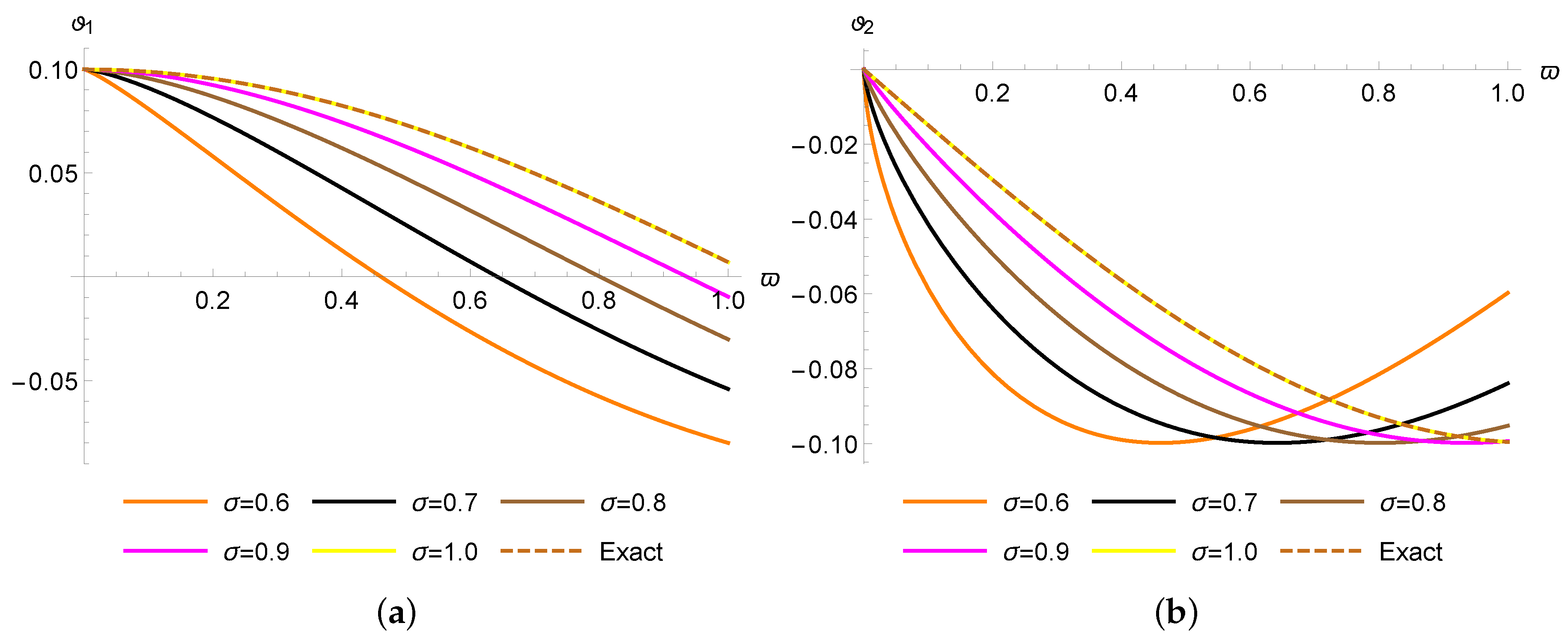
The graphical and numerical results of the App-S and Ex-S for the models shown in Problems 2 and 3 are investigated in this section. The 2D curves of the App-S were extracted from five iterations at $\sigma =0.6,0.7,0.8,0.9,1.0$, and the Ex-S derived via the CSTDM are shown in Figure 1 and Figure 2 of Problems 2 and 3, respectively. When $\sigma \to 1.0$, these figures show how the App-S converged to the Ex-S. The precision and effectiveness of the proposed algorithm were demonstrated by the App-S’s overlap with the Ex-S at $\sigma =1.0$.

Figure 1. The 2D graphs of the App-S and Ex-S of ${\vartheta }_1(\zeta ,\varpi )$ and ${\vartheta }_2(\zeta ,\varpi )$ for various values of $\sigma$ in the range $[0,1.0]$ at $\zeta =0.1$ for Problem 2: (a) ${\vartheta }_1(\zeta ,\varpi )$; (b) ${\vartheta }_2(\zeta ,\varpi )$.

Figure 2. The 2D graphs of the App-S and Ex-S of ${\vartheta }_1(\zeta ,\varpi )$ and ${\vartheta }_2(\zeta ,\varpi )$ for various values of $\sigma$ in the range $[0,1.0]$ at $\zeta =0.1$ for Problem 3: (a) ${\vartheta }_1(\zeta ,\varpi )$; (b) ${\vartheta }_2(\zeta ,\varpi )$.

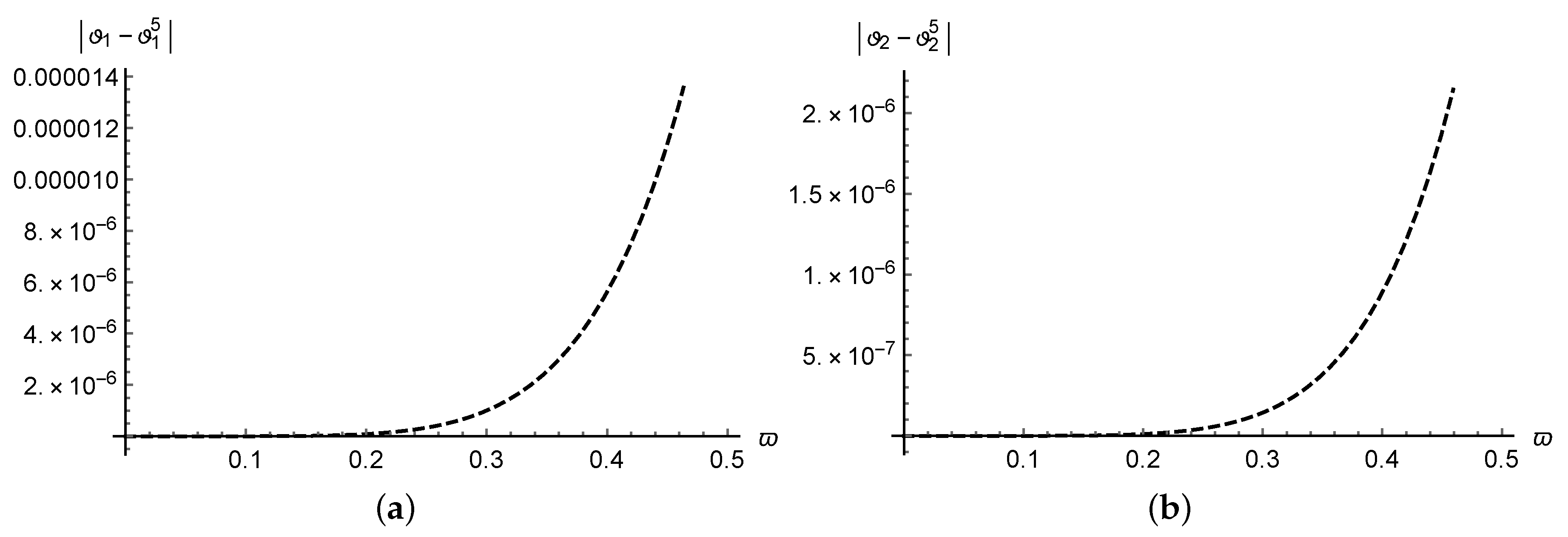
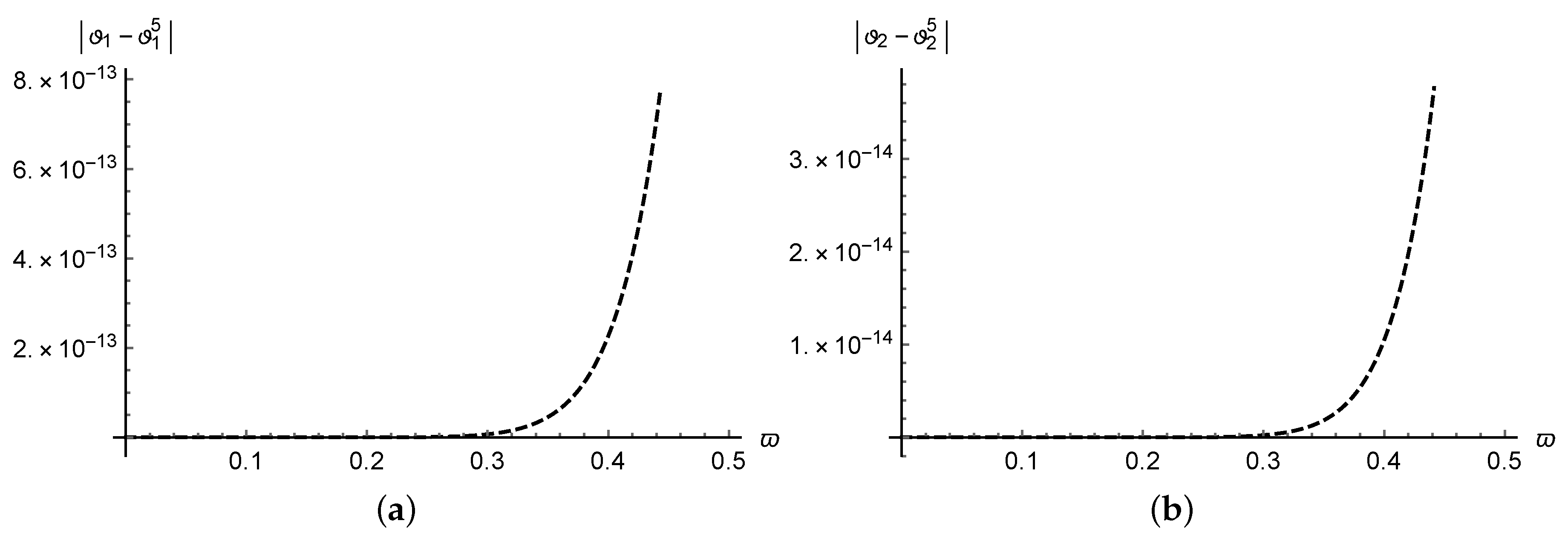
The 2D curve was used to compare the Ex-S and the App-S acquired by five iterations in the sense of the Abs-E obtained using the novel algorithm for Problems 2 and 3 in Figure 3 and Figure 4, respectively. According to the comparison study, the fifth step of the App-S was quite similar to the Ex-S. Therefore, the high precision of the CSTDM was demonstrated by displaying the Abs-E on the graphs.

Figure 3. The 2D graphs of the Abs-E of ${\vartheta }_1(\zeta ,\varpi )$ and ${\vartheta }_2(\zeta ,\varpi )$ for $\sigma =1.0$ in the range $[0,0.5]$ at $\zeta =0.1$ for Problem 2: (a) ${\vartheta }_1(\zeta ,\varpi )$; (b) ${\vartheta }_2(\zeta ,\varpi )$.

Figure 4. The 2D graphs of the Abs-E of ${\vartheta }_1(\zeta ,\varpi )$ and ${\vartheta }_2(\zeta ,\varpi )$ for $\sigma =1.0$ in the range $[0,0.5]$ at $\zeta =0.1$ for Problem 3: (a) ${\vartheta }_1(\zeta ,\varpi )$; (b) ${\vartheta }_2(\zeta ,\varpi )$.

Table 1, Table 2, Table 3 and Table 4 demonstrate the numerical values of the fifth step of the App-S and the Ex-S obtained by the CSTDM to Problems 2 and 3 for various values of fractional order derivatives for selected values of $\varpi$ and $\zeta$ in the intervals $\varpi \in [0,1.0]$ and $\zeta \in [0,1.0]$. These tables show that the App-S approached the Ex-S when $\sigma \to 1.0$. The App-S corresponded with the Ex-S at $\sigma =1.0$, and this proved the effectiveness and precision of the proposed approach.

Table 1. The numerical values of the fifth step of the App-S and the Ex-S to ${\vartheta }_1(\zeta ,\varpi )$ for Problem 2, when $\sigma =0.6,0.7,0.8,0.9,$ and $1.0.$

$(\mathit{\zeta },\mathit{\varpi })$	$\mathit{\sigma }=0.6$	$\mathit{\sigma }=0.7$	$\mathit{\sigma }=0.8$	$\mathit{\sigma }=0.9$	$\mathit{\sigma }=1.0$	$\mathit{Ex}$-S
$(0.1, 0.1)$	$0.8684980$	$0.9267851$	$0.9558931$	$0.9713661$	$0.9800671$	$0.9800671$
$(0.2, 0.2)$	$0.6715970$	$0.7881351$	$0.8551651$	$0.8955971$	$0.9210611$	$0.9210611$
$(0.3, 0.3)$	$0.4456240$	$0.6098471$	$0.7129671$	$0.7800971$	$0.8253370$	$0.8253361$
$(0.4, 0.4)$	$0.2084160$	$0.4066811$	$0.5398871$	$0.6316851$	$0.6967121$	$0.6967071$
$(0.5, 0.5)$	$-0.0268629$	$0.1907591$	$0.3457391$	$0.4577161$	$0.5403210$	$0.5403021$
$(0.6, 0.6)$	$-0.2497790$	$-0.0272871$	$0.1400051$	$0.2660771$	$0.3624081$	$0.3623581$
$(0.7, 0.7)$	$-0.4520310$	$-0.2380731$	$-0.0682092$	$0.0649911$	$0.1700811$	$0.1699671$
$(0.8, 0.8)$	$-0.6272261$	$-0.4334631$	$-0.2703471$	$-0.1372461$	$-0.0289783$	$-0.0291995$
$(0.9, 0.9)$	$-0.7707631$	$-0.6066450$	$-0.4586110$	$-0.3325561$	$-0.226823$	$-0.2272021$

Table 2. The numerical values of the fifth step of the App-S and the Ex-S to ${\vartheta }_2(\zeta ,\varpi )$ for Problem 2, when $\sigma =0.6,0.7,0.8,0.9,$ and $1.0.$

$(\mathit{\zeta },\mathit{\varpi })$	$\mathit{\sigma }=0.6$	$\mathit{\sigma }=0.7$	$\mathit{\sigma }=0.8$	$\mathit{\sigma }=0.9$	$\mathit{\sigma }=1.0$	$\mathit{Ex}$-S
$(0.1, 0.1)$	$0.4957071$	$0.375594$	$0.293716$	$0.2375870$	$0.1986690$	$0.1986691$
$(0.2, 0.2)$	$0.7410210$	$0.6155230$	$0.5183610$	$0.4448681$	$0.3894181$	$0.3894181$
$(0.3, 0.3)$	$0.8955541$	$0.7926010$	$0.7012191$	$0.6256651$	$0.5646430$	$0.5646430$
$(0.4, 0.4)$	$0.9787981$	$0.9137900$	$0.8107160$	$0.7752470$	$0.7173590$	$0.7173560$
$(0.5, 0.5)$	$1.0010701$	$0.9821110$	$0.9384960$	$0.8891591$	$0.8414831$	$0.8414711$
$(0.6, 0.6)$	$0.9707061$	$1.0005310$	$0.9904980$	$0.9640930$	$0.9320801$	$0.9320391$
$(0.7, 0.7)$	$0.8957191$	$0.9728061$	$0.9983310$	$0.9981781$	$0.9855660$	$0.9854560$
$(0.8, 0.8)$	$0.7842271$	$0.9037121$	$0.9639310$	$0.9910961$	$0.9998610$	$0.9995740$
$(0.9, 0.9)$	$0.6444921$	$0.7989421$	$0.8906070$	$0.9440920$	$0.9744760$	$0.9738480$

Table 3. The numerical values of the fifth step of the App-S and the Ex-S to ${\vartheta }_1(\zeta ,\varpi )$ for Problem 3, when $\sigma =0.6,0.7,0.8,0.9,$ and $1.0.$

$(\mathit{\zeta },\mathit{\varpi })$	$\mathit{\sigma }=0.6$	$\mathit{\sigma }=0.7$	$\mathit{\sigma }=0.8$	$\mathit{\sigma }=0.9$	$\mathit{\sigma }=1.0$	$\mathit{Ex}$-S
$(0.1, 0.1)$	$0.0807873$	$0.0908466$	$0.0954577$	$0.0976439$	$0.0987124$	$0.0987124$
$(0.2, 0.2)$	$0.1152671$	$0.1526441$	$0.1726651$	$0.1836350$	$0.1897961$	$0.1897961$
$(0.3, 0.3)$	$0.1032220$	$0.1784380$	$0.2230201$	$0.2497561$	$0.2661000$	$0.2661000$
$(0.4, 0.4)$	$0.0497467$	$0.1667381$	$0.2418071$	$0.2900191$	$0.3214010$	$0.3214010$
$(0.5, 0.5)$	$-0.0376391$	$0.1194070$	$0.2272621$	$0.3005841$	$0.3507901$	$0.3507901$
$(0.6, 0.6)$	$-0.1502061$	$0.04070361$	$0.1801320$	$0.2797700$	$0.3509871$	$0.3509871$
$(0.7, 0.7)$	$-0.2788050$	$-0.0634235$	$0.1032830$	$0.2280010$	$0.3205441$	$0.3205441$
$(0.8, 0.8)$	$-0.4144460$	$-0.1859291$	$0.00129141$	$0.1476601$	$0.2599410$	$0.2599401$
$(0.9, 0.9)$	$-0.5487410$	$-0.3192070$	$-0.1199970$	$0.04284871$	$0.1715541$	$0.1715540$

Table 4. The numerical values of the fifth step of the App-S and the Ex-S to ${\vartheta }_2(\zeta ,\varpi )$ for Problem 3, when $\sigma =0.6,0.7,0.8,0.9,$ and $1.0.$

$(\mathit{\zeta },\mathit{\varpi })$	$\mathit{\sigma }=0.6$	$\mathit{\sigma }=0.7$	$\mathit{\sigma }=0.8$	$\mathit{\sigma }=0.9$	$\mathit{\sigma }=1.0$	$\mathit{Ex}$-S
$(0.1, 0.1)$	$-0.0586526$	$-0.04139580$	$-0.0292325$	$-0.02079380$	$-0.0149189$	$-0.0149189$
$(0.2, 0.2)$	$-0.1618120$	$-0.1271590$	$-0.0982660$	$-0.07581460$	$-0.0587108$	$-0.0587108$
$(0.3, 0.3)$	$-0.2769070$	$-0.2355681$	$-0.1938921$	$-0.1579701$	$-0.1285410$	$-0.1285410$
$(0.4, 0.4)$	$-0.3862281$	$-0.3519160$	$-0.3052460$	$-0.2598771$	$-0.2198820$	$-0.2198820$
$(0.5, 0.5)$	$-0.4779461$	$-0.46431710$	$-0.4221320$	$-0.3734950$	$-0.3267950$	$-0.3267950$
$(0.6, 0.6)$	$-0.5442970$	$-0.5631730$	$-0.5351230$	$-0.4904601$	$-0.4423001$	$-0.4423001$
$(0.7, 0.7)$	$-0.5807641$	$-0.6410880$	$-0.6358610$	$-0.6025191$	$-0.5588090$	$-0.5588090$
$(0.8, 0.8)$	$-0.5855301$	$-0.6928420$	$-0.7173541$	$-0.7019860$	$-0.6686040$	$-0.6686040$
$(0.9, 0.9)$	$-0.5590390$	$-0.715341$	$-0.7742190$	$-0.7820570$	$-0.7643101$	$-0.7643101$

Table 5 and Table 6 show comparisons of the Abs-E of the fifth step of the App-S obtained by the CSTDM in the real $\left({\vartheta }_1(\zeta ,\varpi )\right)$ and imaginary $\left({\vartheta }_2(\zeta ,\varpi )\right)$ parts of Problems 2 and 3 at reasonable nominated grid points in the interval $\varpi \in [0,1.0]$, when $\zeta =0.3$ at $\sigma =1.0$, with the Abs-E of the fifth-step of the App-S being obtained by various approaches, such as the RDTM [30] and the TDDTM [31]. Table 7 and Table 8 show comparisons of the Rel-E of the fith step of the App-S obtained by the CSTDM of the real $\left({\vartheta }_1(\zeta ,\varpi )\right)$ and imaginary $\left({\vartheta }_2(\zeta ,\varpi )\right)$ parts of Problems 2 and 3 at reasonable nominated grid points in the interval $\varpi \in [0,1.0]$, when $\zeta =0.2$ at $\sigma =1.0$ with the Rel-E of the fifth step of the App-S being obtained by various approaches, such as the RDTM [30] and the TDDTM [31]. The comparison confirmed that our approach and the various other approaches produced identical errors. The comparison demonstrated that the CSTDM is a useful substitute tool for the Caputo derivative-based approaches for the solutions of time-fractional QMMs.

Table 5. The absolute errors in different methods for Problem 2 at $\sigma =1.0$.

$\mathit{\varpi }$	${\mathit{\vartheta }}_1(\mathit{\zeta },\mathit{\varpi })$	${\mathit{\vartheta }}_1(\mathit{\zeta },\mathit{\varpi })$	${\mathit{\vartheta }}_2(\mathit{\zeta },\mathit{\varpi })$	${\mathit{\vartheta }}_2(\mathit{\zeta },\mathit{\varpi })$
	[NTHPM]	[30,31]	[NTHPM]	[30,31]
$0.05$	$2.06853\times {10}^{-11}$	$2.06853\times {10}^{-11}$	$6.56092\times {10}^{-12}$	$6.56092\times {10}^{-12}$
$0.15$	$1.50075\times {10}^{-8}$	$1.50075\times {10}^{-8}$	$4.99711\times {10}^{-9}$	$4.99711\times {10}^{-9}$
$0.25$	$3.20003\times {10}^{-7}$	$3.20003\times {10}^{-7}$	$1.11654\times {10}^{-7}$	$1.11654\times {10}^{-7}$
$0.35$	$2.39612\times {10}^{-6}$	$2.39612\times {10}^{-6}$	$8.74607\times {10}^{-7}$	$8.74607\times {10}^{-7}$
$0.45$	$1.07597\times {10}^{-5}$	$1.07597\times {10}^{-5}$	$4.10225\times {10}^{-6}$	$4.10225\times {10}^{-6}$
$0.55$	$3.56416\times {10}^{-5}$	$3.56416\times {10}^{-5}$	$1.41739\times {10}^{-5}$	$1.41739\times {10}^{-5}$
$0.65$	$9.64609\times {10}^{-5}$	$9.64609\times {10}^{-5}$	$3.99607\times {10}^{-5}$	$3.99607\times {10}^{-5}$
$0.75$	$2.23422\times {10}^{-5}$	$2.23422\times {10}^{-5}$	$9.74265\times {10}^{-5}$	$9.74265\times {10}^{-5}$
$0.85$	$4.75409\times {10}^{-4}$	$4.75409\times {10}^{-4}$	$2.12978\times {10}^{-4}$	$2.12978\times {10}^{-4}$
$0.95$	$9.19361\times {10}^{-4}$	$9.19361\times {10}^{-4}$	$4.27625\times {10}^{-4}$	$4.27625\times {10}^{-4}$

Table 6. The absolute errors in different approaches for Problem 3 at $\sigma =1$.

$\mathit{\varpi }$	${\mathit{\vartheta }}_1(\mathit{\zeta },\mathit{\varpi })$	${\mathit{\vartheta }}_1(\mathit{\zeta },\mathit{\varpi })$	${\mathit{\vartheta }}_2(\mathit{\zeta },\mathit{\varpi })$	${\mathit{\vartheta }}_2(\mathit{\zeta },\mathit{\varpi })$
	[CSTDM]	[30,31]	[CSTDM]	[30,31]
$0.05$	$0.0$	$0.0$	$0.0$	$0.0$
$0.15$	$5.55112\times {10}^{-17}$	$5.55112\times {10}^{-17}$	$0.0$	$0.0$
$0.25$	$4.77396\times {10}^{-15}$	$4.77396\times {10}^{-15}$	$1.38778\times {10}^{-16}$	$1.38778\times {10}^{-16}$
$0.35$	$2.70062\times {10}^{-13}$	$2.70062\times {10}^{-13}$	$1.09079\times {10}^{-14}$	$1.09079\times {10}^{-14}$
$0.45$	$5.50562\times {10}^{-12}$	$5.50562\times {10}^{-12}$	$2.85993\times {10}^{-13}$	$2.85993\times {10}^{-13}$
$0.55$	$6.11048\times {10}^{-11}$	$6.11048\times {10}^{-11}$	$3.87976\times {10}^{-12}$	$3.87976\times {10}^{-12}$
$0.65$	$4.52940\times {10}^{-10}$	$4.52940\times {10}^{-10}$	$3.39941\times {10}^{-11}$	$3.39941\times {10}^{-11}$
$0.75$	$2.51806\times {10}^{-9}$	$2.51806\times {10}^{-9}$	$2.18110\times {10}^{-10}$	$2.18110\times {10}^{-10}$
$0.85$	$1.12850\times {10}^{-8}$	$1.12850\times {10}^{-8}$	$1.10811\times {10}^{-9}$	$1.10811\times {10}^{-9}$
$0.95$	$4.27757\times {10}^{-8}$	$4.27757\times {10}^{-8}$	$4.69582\times {10}^{-9}$	$4.69582\times {10}^{-9}$

Table 7. The relative errors in different approaches for Problem 2 at $\sigma =1$.

$\mathit{\varpi }$	${\mathit{\vartheta }}_1(\mathit{\zeta },\mathit{\varpi })$	${\mathit{\vartheta }}_1(\mathit{\zeta },\mathit{\varpi })$	${\mathit{\vartheta }}_2(\mathit{\zeta },\mathit{\varpi })$	${\mathit{\vartheta }}_2(\mathit{\zeta },\mathit{\varpi })$
	[CSTDM]	[30,31]	[CSTDM]	[30,31]
$0.1$	$1.42046\times {10}^{-9}$	$1.42046\times {10}^{-9}$	$29.99334\times {10}^{-10}$	$9.99334\times {10}^{-10}$
$0.2$	$9.39683\times {10}^{-8}$	$9.39683\times {10}^{-8}$	$5.17042\times {10}^{-8}$	$5.17042\times {10}^{-8}$
$0.3$	$1.11911\times {10}^{-6}$	$1.11911\times {10}^{-6}$	$5.07492\times {10}^{-7}$	$5.07492\times {10}^{-7}$
$0.4$	$6.65808\times {10}^{-6}$	$6.65808\times {10}^{-6}$	$2.55892\times {10}^{-6}$	$2.55892\times {10}^{-6}$
$0.5$	$2.72831\times {10}^{-5}$	$2.72831\times {10}^{-5}$	$9.01270\times {10}^{-6}$	$9.01270\times {10}^{-6}$
$0.6$	$8.89954\times {10}^{-5}$	$8.89954\times {10}^{-5}$	$2.53818\times {10}^{-5}$	$2.53818\times {10}^{-5}$
$0.7$	$2.50199\times {10}^{-4}$	$2.50199\times {10}^{-4}$	$6.13872\times {10}^{-6}$	$6.13872\times {10}^{-6}$
$0.8$	$6.37770\times {10}^{-4}$	$6.37770\times {10}^{-4}$	$1.33020\times {10}^{-4}$	$1.33020\times {10}^{-4}$
$0.9$	$1.53085\times {10}^{-3}$	$1.53085\times {10}^{-3}$	$2.65379\times {10}^{-4}$	$2.65379\times {10}^{-4}$
$1.0$	$3.58289\times {10}^{-3}$	$3.58289\times {10}^{-3}$	$4.96586\times {10}^{-4}$	$4.96586\times {10}^{-4}$

Table 8. The relative errors in different approaches for Problem 3 at $\sigma =1$.

$\mathit{\varpi }$	${\mathit{\vartheta }}_1(\mathit{\zeta },\mathit{\varpi })$	${\mathit{\vartheta }}_1(\mathit{\zeta },\mathit{\varpi })$	${\mathit{\vartheta }}_2(\mathit{\zeta },\mathit{\varpi })$	${\mathit{\vartheta }}_2(\mathit{\zeta },\mathit{\varpi })$
	[CSTDM]	[30,31]	[CSTDM]	[30,31]
$0.1$	$1.41294\times {10}^{-16}$	$1.41294\times {10}^{-16}$	$1.16861\times {10}^{-16}$	$1.16861\times {10}^{-16}$
$0.2$	$1.16991\times {10}^{-15}$	$1.16991\times {10}^{-15}$	$0.00000$	$0.00000$
$0.3$	$1.59653\times {10}^{-13}$	$1.59653\times {10}^{-13}$	$1.15629\times {10}^{-14}$	$1.15629\times {10}^{-14}$
$0.4$	$5.49529\times {10}^{-12}$	$5.49529\times {10}^{-12}$	$3.71016\times {10}^{-13}$	$3.71016\times {10}^{-13}$
$0.5$	$7.98778\times {10}^{-11}$	$7.98778\times {10}^{-11}$	$5.58203\times {10}^{-12}$	$5.58203\times {10}^{-12}$
$0.6$	$9.44332\times {10}^{-10}$	$9.44332\times {10}^{-10}$	$5.19106\times {10}^{-11}$	$5.19106\times {10}^{-11}$
$0.7$	$7.48950\times {10}^{-9}$	$7.48950\times {10}^{-9}$	$3.47274\times {10}^{-10}$	$3.47274\times {10}^{-10}$
$0.8$	$5.09649\times {10}^{-8}$	$5.09649\times {10}^{-8}$	$1.83092\times {10}^{-9}$	$1.83092\times {10}^{-9}$
$0.9$	$3.45838\times {10}^{-7}$	$3.45838\times {10}^{-7}$	$8.07183\times {10}^{-9}$	$8.07183\times {10}^{-9}$
$1.0$	$3.78232\times {10}^{-6}$	$3.78232\times {10}^{-6}$	$3.09996\times {10}^{-8}$	$3.09996\times {10}^{-8}$

5. Conclusions

In this research, we have attempted to show whether the CD can serve as a good alternative for the Caputo derivative in the modeling of time-fractional QMMs and in the methods that rely on the Caputo derivative. To do this, we developed an iterative approach based on coupling the CST and the ADM. We also concluded that the CD works well in place of the Caputo derivative for modeling time-fractional QMMs. The graphs and tables show excellent agreement between the App-S and the Ex-S, which demonstrated the highest levels of accuracy of the provided algorithm. The numerical results were also compared with other approaches in the sense of the Abs-E and the Rel-E in which a Caputo derivative was used, such as the RDTM and the TDDTM. The comparison confirmed that our approach and the other mentioned approaches produced identical errors. As a result, we came to the conclusion that the CSTDM is a useful substitute tool for Caputo derivative-based approaches for finding solutions to QMMs. Moreover, we can conclude that the CD is a suitable alternative to the Caputo derivative in the modeling of time-fractional QMMs.

Due to the use of the CST, the pattern between the coefficients of the series solutions made it simple to obtain the Ex-S, and we achieved it in the problems. The use of this approach avoided the need for any problem-related minor or significant physical parameter assumptions. As a result, it bypassed some of the limitations of traditional perturbation approaches and could be used to solve both weakly and strongly nonlinear problems. In contrast to earlier approaches, the CSTDM could produce series solutions for both linear and nonlinear FDEs without the use of perturbation, linearization, or discretization steps. Solving QMMs requires only a minimal number of computations. Hence, the power of this algorithm lies in the efficiency of its computations. The CSTDM provides an approximate analytical solution in terms of an infinite fractional power series. In this study, we determined five terms of the series, which was enough to approximate the exact solution, which we proved both graphically and numerically.

As a result of the findings, we conclude that the CSTDM is a simple-to-use and accurate tool to solve fractional order differential equations. The limitation of this approach is that to achieve the solution in the original space, the CSTDM must first determine the CST of the target equations and then execute the inverse CST. Therefore, the source functions for nonhomogeneous equations must be piecewise continuous and of exponential order, and, after the calculations, the inverse CST must exist. In the future, we hope to apply the CSTDM to other fractional order differential equation systems that arise in other fields of science.