Appendix A. Graphene Parameters
The optical properties of graphene can be determined by the surface conductivity
, which describes the interaction between graphene with electromagnetic radiation and can be given by Drude’s semi-classical model [
37]:
where
is the Drude weight,
is the minimum conductivity of graphene,
eV is the Fermi energy of graphene,
ℏ is the reduced Planck’s constant,
e is the electron charge,
ps is the relaxation time,
1/s and
is frequency of the incident electromagnetic wave.
Application of the external magnetic field
leads to the circulation of charge carriers in graphene in cyclotron orbits due to the Lorentz force. In this case, the 2D conductivity tensor of graphene with non-zero off-diagonal components can be described by [
37]
where
is the cyclotron frequency,
m/s is the Fermi velocity, and
and
are the longitudinal (diagonal) and transverse (off-diagonal) parts, respectively. For the device operating the THz frequency range, we consider only the intraband contributions for the calculation of the components of the graphene conductivity tensor [
]. The influence of interband transitions can be neglected, since the condition
is satisfied [
38].
Appendix B. Elements of Magnetic Group Theory
Time reversal operator. The time reversal
T, which changes the sign of the time, and its combination with geometrical symmetry elements are called the antiunitary operators [
1]. The time reversal operator reverses the direction of currents, magnetic fields, and the Poynting vector. In the frequency domain, it also conjugates electromagnetic quantities and this property can be shown easily by the Fourier transform of the time-reversed quantities [
21].
It should be stressed that due to causality, the time-reversal symmetries in physical processes do not exist. Moreover, the dissipative processes are not time-reversible. A modified version of this operator called the restricted time reversal operator was suggested in [
21]. It is not applied to the dissipative terms of the electromagnetic quantities preserving thus the passive or active nature of the media.
Categories of magnetic groups. The magnetic groups can be divided into three categories. The group of the first category G presents a unitary subgroup H and products of the time reversal with the elements of H. The magnetic groups of the second category do not contain time reversal T. The notations of the groups of the first category and those of the second category coincide. In order to distinguish them, we use the bold-face type for the groups of the second category.
The groups of the third category
, which are the most interesting for us, have the so-called antiunitary elements, which present the product of
T and the geometrical symmetry elements. We call these elements antielements (for example, antiplane of symmetry). The group of the third category can be described as
. These groups can be defined also in a different way, namely,
, where
B is any antiunitary element of group
G. A description of these categories of magnetic groups is given in
Table A1
Table A1.
Content of magnetic groups of symmetry.
Table A1.
Content of magnetic groups of symmetry.
| First Category | Second Category | Third Category |
|---|
| G | |
| including T | without T | T only in combination |
| | | with rotation-reflections |
Co-representations. Wigner [
1] introduced in the group theory the so-called corepresentations where the term “corepresentation” reminds one of the complex conjugate signs in the matrix multiplication scheme [see (
A7) below]. The corepresentations are defined as follows:
where
and
a are antiunitary elements,
u is a unitary one,
is an irreducible representation of
H.
Homomorphism scheme. The multiplication scheme for corepresentations in the group of the third category, for
unitaries and
anti-unitaries, is as follows:
Herring rule. This rule [
35] defines three special cases:
where
is the subgroup order,
is the character of corepresentation
, where
a is an antiunitary element. This rule permits determining the reducibility of the corepresentation. For our purposes, this rule can be read as follows. In case (a), no new degeneracy is introduced; in case (b), the degeneracy of
is doubled, i.e., a given representation appears twice and the eigenvectors are different and orthogonal but the eigenvalues are identical; in case (c), the representation
is degenerate with the representation
, i.e., a pair of different eigenvectors has the same eigenvalue. Hence, in case (a), we may discuss the problem of the degeneracy of group
, investigating only the unitary subgroup
H. In case (b), the degeneracy of one of the eigenvalues appears, though this degeneracy is absent in subgroup
H. In case (c), the degeneracy of two different eigenvectors exists, though it is also not predicted by subgroup
H (see
Appendix E).
Projection operator. In order to obtain SALCs in the case of a magnetic group of the third category, we use the projection operator [
39], which for 2D ICR is written as follows:
where the summation in the first sum is over the unitary elements
u, and in the second sum is over the antiunitary ones
a,
are elements of the corepresentation.
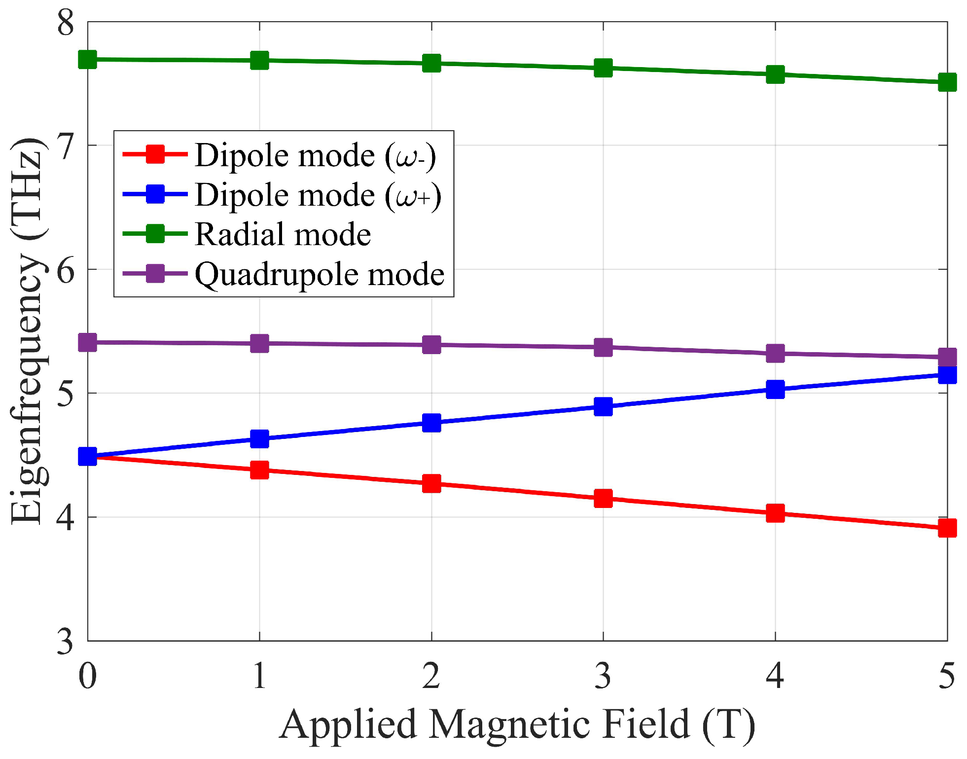
Appendix C. Splitting of IR E of in
The field
removes the degeneracy which exists in the square non-magnetized structure due to the representation
E. In order to find the representations of the
group, which are contained in the representation
E of
, we write out the characters (i.e., traces of the IR) of
Table 2 for IR
E corresponding to the operations of the
group. It is presented in
Table A2.
Table A2.
Characters of the irreducible representation E of group .
Table A2.
Characters of the irreducible representation E of group .
| e | | | |
| E | 2 | −2 | 0 | 0 |
The number of times
a given IR
appears in the reducible representation is defined by the following relation:
where
is the character of the reducible representation,
is the character of the irreducible representation. Using this formula, we find:
Therefore, the representation
E of
of the non-magnetized waveguide splits into the representations
and
of the unitary
subgroup of the magnetized waveguide. The results are presented in
Table A3. Many tables of this type are given in [
32].
Table A3.
Symmetry degeneration of group in and .
Table A3.
Symmetry degeneration of group in and .
| , Table 2 | , Table A5 | , Table 5 |
| | |
| | |
| | |
| | |
| E | , | , |
Appendix D. The 2D Eigenvectors of Cases and
In the microwave circuit wave theory [
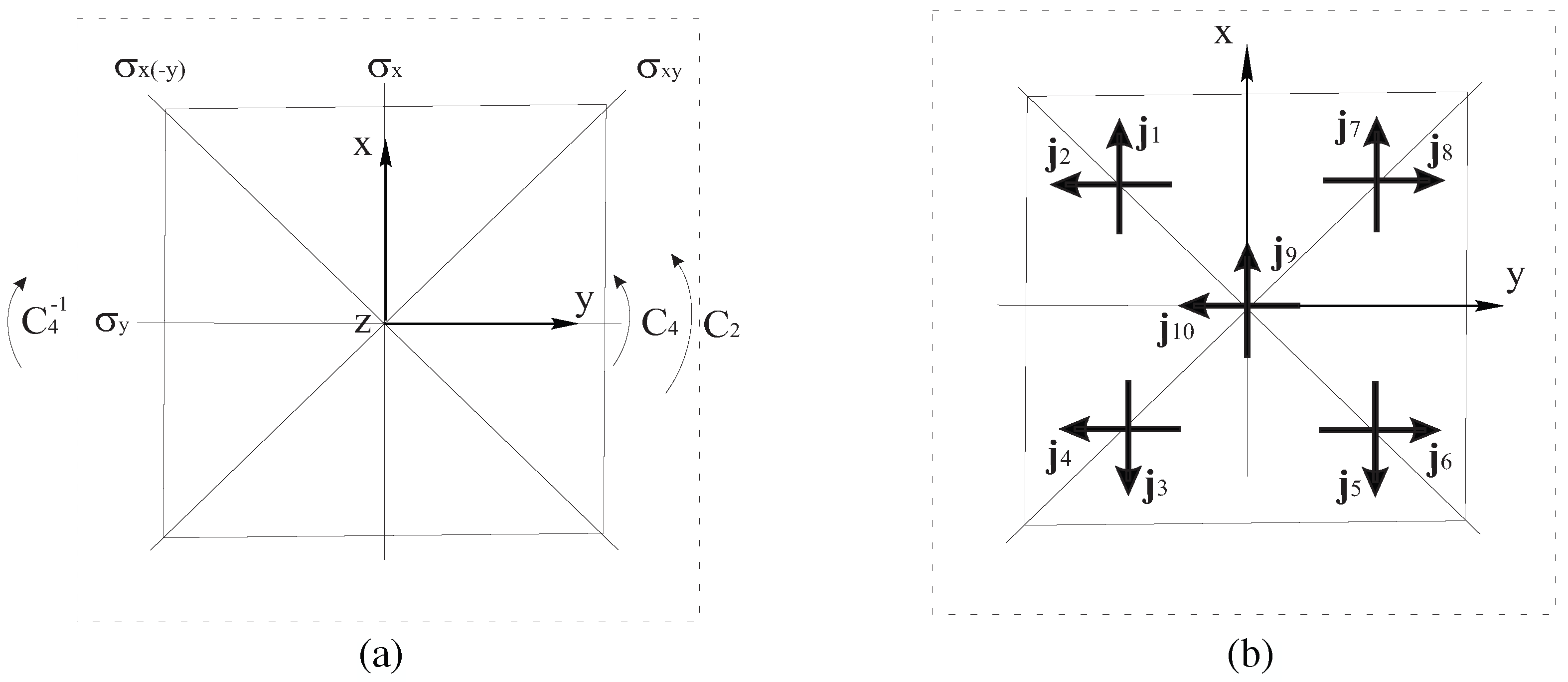
36], one deals with voltage waves. In 2D vector space
(see
Figure 1), the two-component eigenvectors (wave vectors)
and
of the incident wave in port 1 and port 2 can be written as follows
In the symmetry
, these two modes are degenerate because they belong to the 2D IR
E. Under symmetry operators, they are transformed into each other or themselves. For example, the operator
applied to
and
gives
i.e., the basis vector
is transformed into
and
is transformed into
. Hence, due to the square form of the unit cell, we deal with the 2D polarization degeneracy.
Any linear combination of the two degenerate eigenvectors
and
, for example,
is also an eigenvector. This combined vector is transformed also according to the 2D IR
E of
Table 2.
Now we shall find the symmetry-adapted 2D voltage wave vectors of our magnetized structure with magnetic symmetry
. Using the projection operator (
A9) of
Appendix B for the 1D representation
of group
and choosing
of (
A15) as an arbitrary vector
, we obtain:
In Equation (
A18),
,
,
,
. This equation can be explained as follows. The operator
e preserves the vector
and
, so that the first term of the sum is
. The operator
changes the sign of
, i.e.,
. With
, the second term becomes
. The operator
transforms the vector
into
and
. As a result, we obtain the third term
. The last term of the sum is
.
Analogously, for the representation
, we can write:
After normalization, vectors (
A18) and (
A19) take the following form:
The vectors in (
A20) describe two circularly polarized modes in the polar representation (rotating basis). They are also eigenvectors of the non-magnetized structure. However, unlike the non-magnetized array with symmetry
, vectors
and
are not degenerate because they belong to different 1D representations of
.
Appendix E. Example of Degeneracy Due to Case (C) of (A8), Group
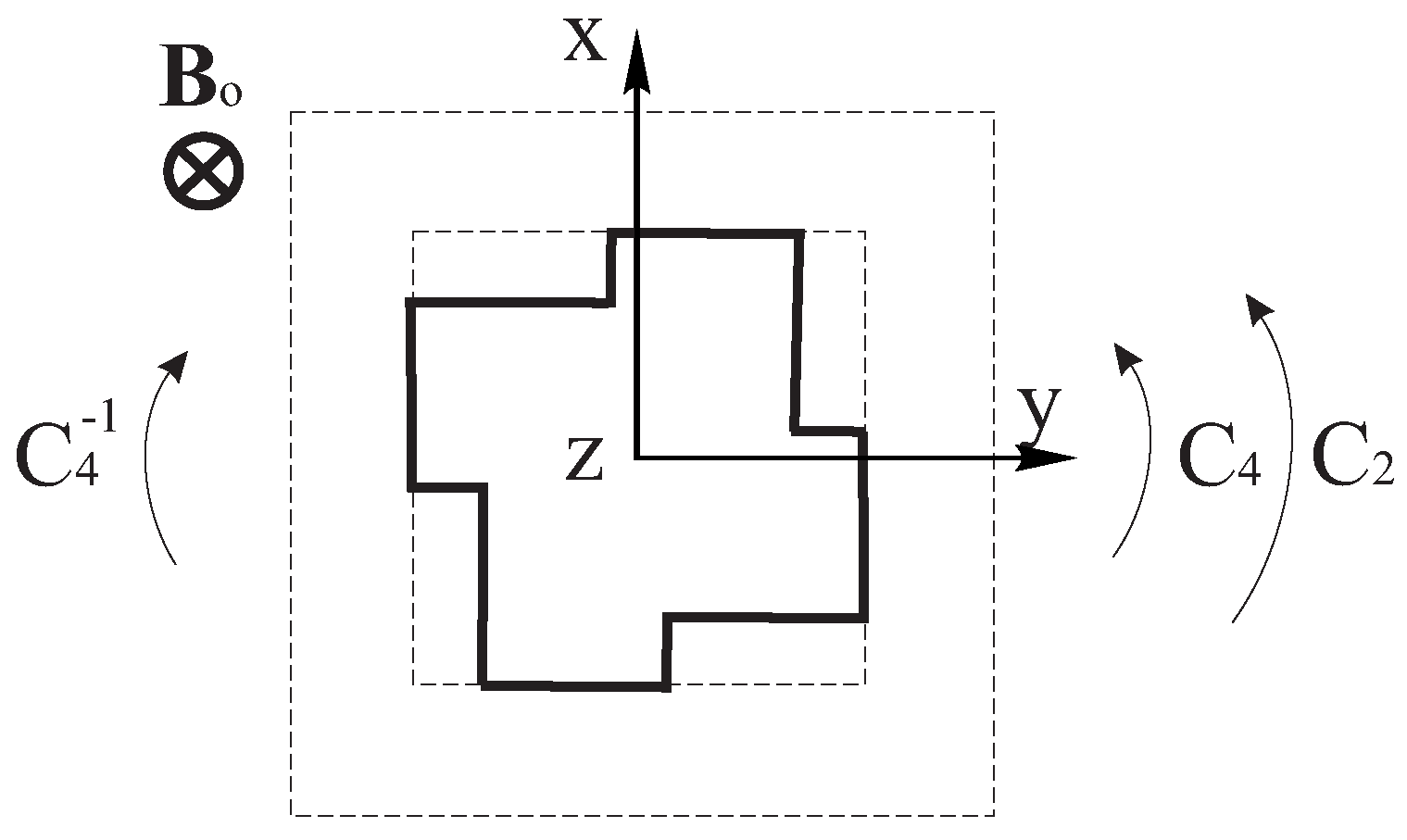
Now we apply it to an object with another magnetic symmetry. In the microwave region, a square metal waveguide filled with ferrite and magnetized by a quadrupole DC magnetic field (
Figure A1), as presented in [
40]. Here, we discuss this structure from the point of view of the magnetic group theory and Herring rule.
In the nonmagnetic case with symmetry
, the two-component eigenvectors
and
of the incident wave in port 1 and port 2 are given by (
A15).
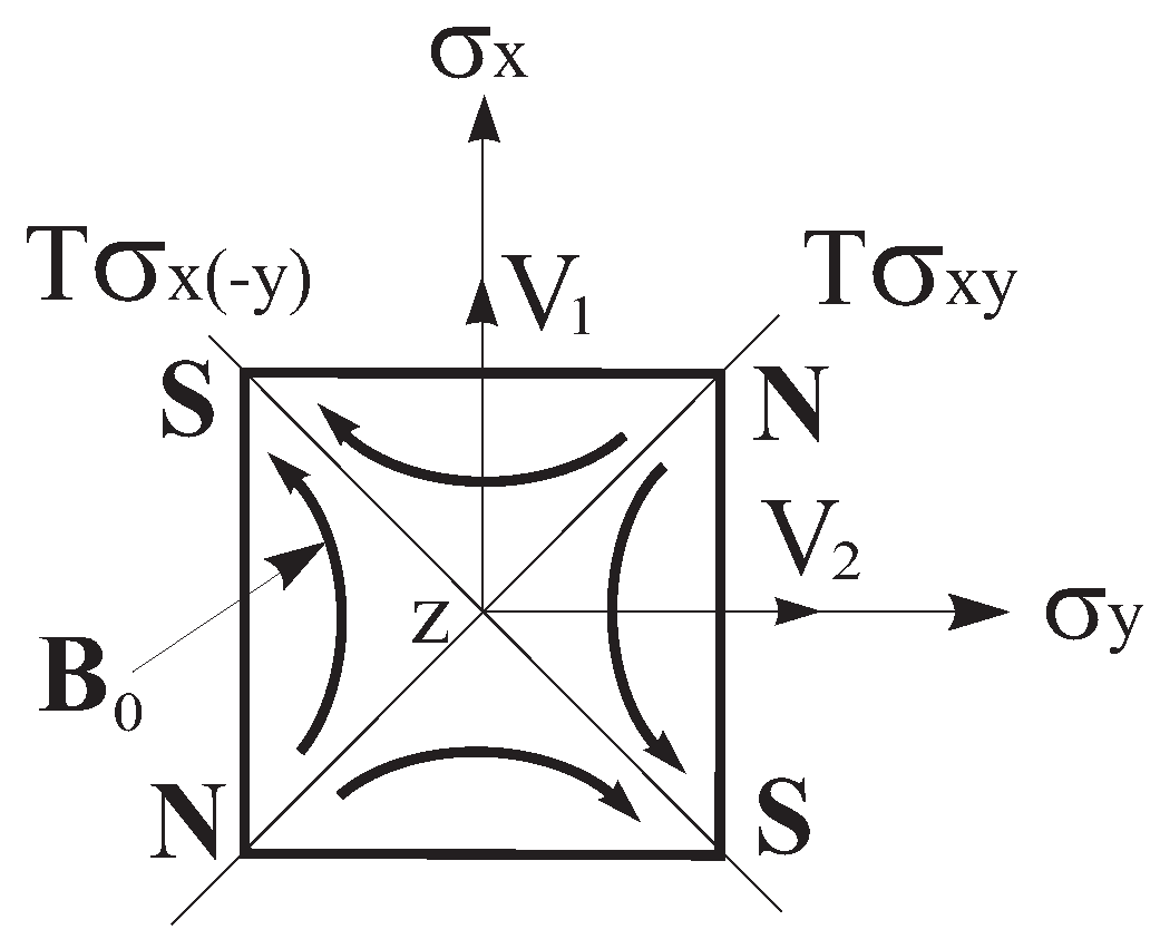
Figure A1.
Cross-section of square metal waveguide with ferrite. Magnetization by a quadrupole DC magnetic field , , and are the poles of the magnet system. and are planes of symmetry, and are antiplanes of symmetry.
Figure A1.
Cross-section of square metal waveguide with ferrite. Magnetization by a quadrupole DC magnetic field , , and are the poles of the magnet system. and are planes of symmetry, and are antiplanes of symmetry.
In the magnetic case with the quadrupole field
, the magnetic group of the third category is
. The degeneracy of
in
is presented in
Table A3. The ICRs
and
of this group are given in
Table A4. It is case (c) of (
A8). The ICRs
and
are equivalent because they can be transformed one into another by a unitary matrix.
Considering
as an independent group of the first category, we see from
Table A5 that no degeneracy is predicted by this group because all of its representations are 1D. The symmetry
describes, for example, the rectangular waveguide. The polarization degeneracy in the rectangular waveguide is impossible. Summarizing, the square waveguide with isotropic medium with the symmetry
has the polarization degeneracy described by vectors (
A15), and the rectangular waveguide with the symmetry
does not have such a degeneracy, but the magnetic square waveguide with the symmetry
has a degeneracy again. However, the latter degeneracy differs from that of the isotropic square waveguide.
Table A4.
Irreducible corepresentations and of group , .
Table A4.
Irreducible corepresentations and of group , .
| e | | | | | | | |
| | | | | | | | |
| | | | | | | | |
Table A5.
Irreducible representations of group .
Table A5.
Irreducible representations of group .
| e | | | |
| 1 | 1 | 1 | 1 |
| 1 | 1 | | |
| 1 | | 1 | |
| 1 | | | 1 |
It is easy to show that the vectors (
A15) in the symmetry
are not degenerate in the usual sense as it was in the case of the nonmagnetic square waveguide. The antiunitary operators of
Table A4 change the sign of the wave vector
(see
Table 1). Under these operators, the vector
is transformed into the vector
and vice versa. It means that these two vectors are degenerate if we consider wave
propagating in one direction in the waveguide and wave
propagating in the opposite direction. A two-component vector is transformed in accordance with 2D IRCs
and
of
Table A4. The overall parameter
in the antiunitary operators defines a possible phase shift between the forward and backward waves, i.e., a nonreciprocal phase shift. In our 2D description, this parameter is not defined. If we include into consideration the third coordinate, and there exists the two-fold rotation symmetry with the axis
, it gives
, and vectors
and
are interchanged under this operator, i.e., it corresponds to degeneracy and the parameter
can be equal to 1. Thus, one can see that this case with
is quite different from the one discussed in the main part of the paper case with
.


