The Impact of Connected and Autonomous Vehicle Platoon’s Length on Expressway Traffic Flow Characteristics Based on Symmetry Lane Changing Rules

Abstract

This study mainly investigates the maximum length of CAV (Connected and Autonomous Vehicle) platoons in a heterogeneous traffic flow environment. By employing MATLAB to simulate the heterogeneous traffic flow on expressways, this study focuses on the maximum platoon length of CAV platoons and explores their impact on the traffic flow characteristics on expressways. Firstly, based on four different car-following modes of heterogeneous traffic flow, F-STCA (Flexible–Symmetric Two-Lane Cellular Automata Model) and the symmetric lane-changing strategy, the study refines and improves the construction of the NaSch (Nagel and Schreckenberg) model introduced into the Gipps safety distance formula. The whole improvement process is based on the acceleration decay characteristics of vehicles on expressway. Secondly, the congestion situations under different maximum platoon lengths are compared using fundamental heat maps of the simulation data. The evolution of the fundamental diagram with changes in maximum platoon length is studied to investigate the impact and magnitude of maximum platoon lengths on the road capacity under different CAV permeabilities. Finally, the study explores the stability and safety of heterogeneous traffic flow involving CAV platoons using SD (Standard Deviation) and TERCRI (Time-Exposed Rear-End Collision Risk Index). The results show that when the CAV’s permeability does not reach a high level on heavily trafficked sections of the expressway, considering the overall average speed, the maximum platoon length should not be set too long and should be around five vehicles. This restriction does not apply when the CAV permeability approaches 100%.

1. Introduction

Taking a comprehensive view of the current research on traffic flow-following models, car-following models from the traffic engineering perspective focus on describing the micro-behavior of the driver [1,2,3,4,5,6,7]; these car-following models are represented by stimulus response class models such as General Motors’ (GM), safety distance models such as Gipps’, psychophysiological models such as Wiedemann’s, and artificial intelligence models. However, car-following models from statistical physics perspectives, represented by models such as Optimized Velocity Models (OVM), the Intelligent Driver Model (IDM) and NaSch Cellular Automata models, focus on describing the meso and macro traffic characteristics, using simple models to describe micro driving behaviors, and to reveal the complex dynamics and characteristics of traffic flow [8,9,10,11,12]. Cellular Automata (CA) models originated from Wolfram’s Rule 184 [13], after the development and evolution of the NaSch model [14], FI model [15] and VDR model [16]. CA involves a large number of mature and improved models. Since the lane-changing model was first proposed [17,18,19], the probability of lane-changing has been considered and random error has been introduced [20]; three kinds of lane-changing behavior have been classified [21], and another kind of probability model based on utility choice theory has been introduced [22,23]. In terms of improving the traditional model, Wang et al. [24] proposed a car-following model for unsignalized intersections in the V2V environment. In terms of improving traditional models, Wang et al. proposed a car-following model for signal-free intersections in V2V environments [24]. TANG et al. proposed an improved model to overcome the deficiencies of full-velocity difference models in collision accidents [25]. Ou et al. applied the improved model to analyze the operating conditions of vehicles in a dual-lane traffic system during accidents [26]. Regarding lane changing models, Wang Yongming et al. [27] proposed the concept of elastic safe lane-changing distance based on Chowdhury’s [28] Symmetric Dual-Lane Cellular Automata Model (STCA), and designed the corresponding dual-lane CA model F-STCA [29].

Besides this, in the research on automated expressway systems, car-following models such as constant spacing strategy [30] have been proposed, but automated highway systems (AHSs) mainly focus on autonomous driving and do not involve connected and autonomous technology. Currently, research in the field of Vehicle Automation and Communication Systems (VACS) includes Cooperative Adaptive Cruise Control (CACC) systems in V2V environments [31] and intelligent speed regulation systems in V2I environments [32]. The early CACC concept was developed by Tampere et al. [33]. CACC allows vehicles to actively communicate and coordinate with preceding vehicles or multiple vehicles ahead to adjust their speed, significantly reducing the inter-vehicle spacing [34]. As an extension of connected cruise control, vehicles under CACC can coordinate their acceleration by obtaining the acceleration of the preceding vehicle [35]. Since the participation of connected and autonomous vehicles (hereafter referred to as CAVs) in the research on heterogeneous traffic flow characteristics, studies on the effects of different proportions of vehicle types on congestion relief [36] have gradually increased. V2I technology combined with the variable speed limits method enables real-time adjustments of vehicle speed, and can achieve objectives such as congestion relief or fuel consumption reduction [37]. Milanés et al. [38] proposed a car-following model equipped with Adaptive Cruise Control (ACC) and CACC technology based on parameters such as the error between the actual inter-vehicle spacing and the desired spacing, the weight of the inter-vehicle spacing error, the weight of the velocity difference, and the derivative weight of the inter-vehicle spacing error. Marzoug R et al. [39] proposed a cellular automata model to investigate the different traffic emissions (CO2, PM, VOC, and NOx) and speeds at a two-lane signalized intersection. The model is designed to analyze the effects of signalization by isolating the parameters involved in vehicle–vehicle interactions (lane changing, speed, density, and traffic heterogeneity).

Currently, most of the research on microscopic traffic simulation models based on connected and autonomous technology is built upon existing traffic flow models, combined with assumptions about the operational characteristics of CAVs. Regarding the following characteristics of heterogeneous traffic flow, the existing studies mainly approach analysis using single-type car-following models [40,41,42,43,44,45,46,47,48]. Li et al. [49] proposed a following model based on multiple headway, velocity difference, and acceleration difference. Zhu et al. [50] studied the fundamental diagrams and density waves of heterogenous traffic flow with manual and autonomous driving. Jiang et al. [51] used the Full Velocity Difference (FVD) model and CACC model to describe the following characteristics of human driving vehicles (hereafter referred to as HDVs) and CAVs, and analyzed the linear stability and safety of heterogenous traffic flow. In addition, research on the following characteristics of heterogeneous traffic flow under different following modes has also become a topical issue in recent years [52]. Wang Y, Jiang Y, Wu Y, et al. [53] proposed a control strategy for CAVs that considers the driving behavior of CAVs platoons based on the FS strategy, which allows CAVs to execute the FS strategy as a platoon. Then, a cellular automaton model of mixed traffic flow was developed based on the proposed strategy.

Furthermore, there has been a large number of global research achievements made in the field of CAV platoons in recent years. Marcel Sala et al. [54] estimated the average length of a platoon under given traffic demand and different permeability rates by providing a generalized macroscopic model, comparing two different platoon arrangements based on cooperation or opportunity, representing the optimal and worst-case scenarios, respectively. Francisco Nava et al. [55] proposed a novel Advanced Cooperative Adaptive Cruise Control (ACACC) that utilizes existing communication with the preceding vehicle to reduce the gap between vehicles while maintaining vehicle stability. Liling Zhu et al. [56] proposed a heterogeneous traffic flow model of platoons and regular vehicles based on CA, analyzing the impact of platoon permeability rate and platoon size on road capacity, traffic congestion, and lane-changing frequency. Linjie Zhou et al. [57] proposed four types of heterogeneous traffic flow configurations and distribution characteristics, provided the fundamental schematic diagrams considering the degradation of CACC system and the formation of CAVs, and discussed the impacts of degraded CAV platoons’ control modes on the fundamental diagrams. Zhen Wang et al. [58] proposed a dynamic cooperative lane-changing model for autonomous driving cars considering the preceding vehicles’ acceleration, updating the target vehicles’ lane-changing decisions in real-time through lane-changing decisions, cooperative trajectory planning, and trajectory tracking. Shuke An et al. [59] proposed a discrete following interval model for autonomous driving cars, including steady-state following interval and dynamic following interval, to study the stability of heterogeneous traffic flow. Zhihong Yao et al. [60] considered that following an HDV in heterogeneous traffic flow would impair the performance of CAVs due to different reaction times between different following relations, and based on this, the linear stability of such non-uniform traffic flow was derived and analyzed.

At the same time, when we are tracking the latest research in the field, we see a significant amount of studies focusing on the platooning of CAVs in the heterogeneous traffic flow. Of these, various studies have demonstrated the optimal length of platoons based on experimental data. Some studies suggest that with the increase in the length of the platoon, the traffic capacity increases, the congestion rate alleviates, and the lane-changing frequency reduces; however, the effect is no longer obvious when it reaches a certain threshold [56]. There are also studies that indicate, when the permeability rate of motor vehicles is 100%, that increasing the maximum platoon length can enhance the traffic capacity of the road. In a certain density range, the maximum platoon length has an optimal value [61].

It can be seen that with the continuous development of heterogeneous traffic flow modeling that considers a platoon of vehicles, the research on maximum platoon length has become the latest topical issue. However, there is still no unified research perspective and standardized definition in this field, and the conclusions of studies on the optimal value of the maximum platoon length vary. This paper aims to investigate the impact of maximum platoon length on traffic flow with simultaneous variations in multiple dimensions and influencing factors by improving the model and conducting many simulation experiments. The main contributions of this study to the literature are as follows: Firstly, it studies the impact of the maximum platoon length of CAV platoons on traffic flow in heterogeneous traffic environments involving CAVs. By analyzing the car-following characteristics of vehicle platoons and symmetric lane-changing mechanisms, we can improve the model to construct a detailed, scientific, and effective simulation model for heterogeneous traffic flow of CAVs, providing the means for undertaking such studies on heterogeneous traffic flow. Secondly, by changing the simulation environment from the six permeabilities of CAVs, 20 density settings of traffic flow, and 10 maximum platoon lengths, a large number of simulation experiments can be conducted on the above 1200 combinations, providing a credible foundation of data for this research and similar studies. Thirdly, the study considers the length of CAV platoons, focusing on the corresponding changes in traffic flow characteristics when the maximum platoon length changes, as well as the degrees and patterns of this influential capacity as affected by other factors. The study explores the optimal value of the maximum platoon length of CAV platoons under different permeabilities and density environments, providing a basis for the future rational organization and traffic management of CAV platoons.

2. The Model

2.1. CA Model of Heterogeneous Traffic Flow on Expressway Involving CAV Platoons

2.1.1. Cellular Automata Model Based on Gipps Safety Distance Formula

In this study, factors such as safety distance, randomization probability, and platoon behavior were considered, distinguishing CAVs from HDVs and four types of car-following modes. In addition, when combined with the classic Gipps model, this study introduces the concept of “safety distance” to improve the NaSch model, and a car-following model for CAVs based on Gipps safety distance has been established [61].

Based on the principle of calculating safety distance, the safety distance constraint is obtained:

$$x_{n-1}(t)+\frac{v_{n-1}{(t)}^2}{2b_{n-1}}-l_{n-1}\ge x_n(t)+v_n(t){\tau }_n+\frac{v_n{(t)}^2}{2b_n}$$

(1)

where τ_n is the reaction time of vehicle n; l_n−1 is the length of the preceding vehicle of vehicle n; v_n(t) and v_n−1(t) are, respectively, the speed of vehicle n and its preceding vehicle at time t; x_n(t) and x_n−1(t) are, respectively, the position of vehicle n and its preceding vehicle at time t; b_n and b_n−1 are, respectively, the maximum deceleration of vehicle n and its preceding vehicle.

The safe following distance, d_n,safe, is the safety distance that the following vehicles should maintain when the lead vehicle engages in emergency braking maneuvers, primarily represented by the reaction time in this study. The calculation formula of safety distance d_n,safe, required by the nth vehicle during driving at time t, is as follows:

$$d_{n,safe}(t)=x_{n-1}(t)-x_n(t)-l_{n-1}=v_n(t){\tau }_n+\frac{v_n{(t)}^2}{2b_n}-\frac{v_{n-1}{(t)}^2}{2b_{n-1}}$$

(2)

According to the safety distance calculation Formula (2), the safe speed v_safe,n used by the vehicle to avoid collision can be obtained, and the calculation formula is as follows:

$$v_{safe,n}(t)=-b_n{\tau }_n+\sqrt{b_n^2{\tau }_n^2+b_n\left\{2d_n-{\tau }_n{v}_n(t)+\frac{v_{n-1}^2(t)}{b_{n-1}}\right\}}$$

(3)

where d_n is the distance between the nth vehicle and the previous vehicle n−1:

$$d_n=x_{n-1}\left(t\right)-x_n\left(t\right)-l_{n-1}$$

(4)

2.1.2. CA Model in Heterogeneous Traffic Flow

Based on determining the safety distance d_n,safe and the safe speed v_safe,n, the vehicle is restricted by the following speed and position evolution rules.

• Acceleration

When the distance d_n between the nth vehicle and the vehicle in front of it (the n−1 car) is greater than its required distance d_n,safe, the nth vehicle is more inclined to drive at a higher speed and accelerate according to

$$v_n(t+1)=\min \left\{\begin{array}{c}{v}_n(t)+a_n(t+1)\\ V_{\max }\\ d_n\\ v_{safe,n}(t)\end{array}\right.,d_n>d_{n,safe}$$

(5)

where a_n(t + 1) is the acceleration of the next time step of the nth car. This study has refined the model by considering the acceleration reduction characteristics of high-speed vehicles, introduced into the acceleration reduction the parameter a_n,red, and made changes to a_n in the “Acceleration” as

$$a_{n,red}(t)=\left\{\begin{array}{cc}0& v_n(t)\le 60\mathrm{km}/\mathrm{h}\\ 0.1\times ⌈\frac{v_n(t)-60}{10}⌉& 60\mathrm{km}/\mathrm{h}<v_n(t)\le 120\mathrm{km}/\mathrm{h}\end{array}\right\}$$

(6)

$$a_n(t+1)=a_n-a_{n,red}(t)$$

(7)

where v_n(t + 1) is the speed of vehicle n at time t + 1; V_max is the maximum speed of the vehicle; a_n and a_n,red(t) are, respectively, the maximum acceleration of vehicle n and its acceleration attenuation at time t.

• Deceleration

When the inter-vehicle distance d_n is less than the minimum safety distance d_n,safe, the vehicle decelerates according to the following rules for safety considerations:

① When the front vehicle is stationary, the vehicle adopts safety deceleration rules—

$$v_n(t+1)=\max \left\{\begin{array}{c}\min \left(v_{safe,n}(t),d_n-1\right)\\ 0\end{array}\right.,v_{n-1}(t)=0\wedge d_n<d_{n,safe}$$

(8)

② When the front vehicle is not stationary, the vehicle adopts deterministic deceleration rules—

$$v_n(t+1)=\max \left\{\begin{array}{c}\min \left(v_{safe,n}(t),d_n\right)\\ 0\end{array}\right.,v_{n-1}(t)\ne 0\wedge d_n<d_{n,safe}$$

(9)

• Uniform Velocity

When d_n = d_n,safe, the vehicles travel at uniform velocity, and the rule is as follows:

$$v_n(t+1)=\min \left(v_n(t),d_n\right),d_n=d_{n,safe}$$

(10)

• Randomization

There are uncertain factors affecting the driving process, which cause some vehicles to decelerate. Therefore, the HDVs with ρ_slow probability in the model perform random slowing according to these rules, while the CAVs do not participate in the slowing process.

$$v_n(t+1)=\max \left(v_n(t)-b^{\prime }{}_n,0\right),p_{n,rand}(t)\le {\rho }_{slow}$$

(11)

where b′_n is the normal deceleration of vehicle n; p_n,rand(t) is the real number vehicle n randomly generates between 0 and 1 at time t; ρ_slow is the randomization probability.

• Location update

After the evolution of vehicle speed over unit time, the vehicle position adopts the following updating rules:

$$x_n(t+1)=x_n(t)+v_n(t+1)$$

(12)

Based on the above model, when CAV follows CAV, due to the ability of vehicles within the CAV platoons to travel with smaller inter-vehicle distances, in the formation process of platoons, the other vehicles in the team aside from the lead vehicle execute d_n,safe acceleration (Formulas (5)–(7)), deceleration (Formulas (8) and (9)), and uniform velocity (Formula (10)) rules, with a fixed value of 3 m.

After the formation of a platoon, when the vehicles inside the platoon reach uniform velocity, that is, when the inter-vehicle distance between the nth vehicle and its predecessor is equal to 3 m, the two cars become a stable platoon, and the nth vehicle adopts the same driving behavior as its predecessor. The evolution rules are as follows:

$$v_n(t+1)=v_{n-1}(t+1),d_n=d_{n,safe}=3\mathrm{m}$$

(13)

In this case, the vehicles are CAVs, and there is no random slowing process. Therefore, after the speed of the vehicle is obtained, its position is updated using Formula (12). If the d_n,safe of the lead vehicle changes, all the vehicles in the platoon will adopt the evolution rules described in Formulas (5)–(10) to change their driving behavior until a stable platoon is formed again.

2.2. Lane-Changing Model in Traffic Flow on Expressway with the Participation of CAV Platoons

2.2.1. Lane-Changing Model of Dual-Lane Manual-Driving Vehicles

Under manual driving conditions, only when the driver is driven by some motives will he have the willingness to change lanes, and then make the decision to change lanes. Under the manual-driving behavior, drivers can only roughly estimate the speed of the vehicle approaching behind, and cannot predict the speed change of the vehicle approaching in next in advance. In the improved F-STCA model, the acceleration value “1” in the original model is replaced by acceleration parameter an to consider the acceleration performance of the vehicle itself [29]. On this basis, in order to ensure the safety of the lane-changing process, the constraints on d_n,back in the safety conditions of the F-STCA model are improved:

$$\left\{\begin{array}{c}{d}_{n,back}>d_{\sigma }+v_{\max }-\min (v_n+a_n,v_{\max })\\ d_{\sigma }\ge 1\end{array}\right.$$

(14)

It should be mentioned that lane-changing behavior can be divided into symmetric lane-changing and asymmetric lane-changing according to the changing mechanism. Symmetric lane-changing adopts the same lane-changing strategy regardless of whether a vehicle is in the left lane or the right. Asymmetric lane-changing implies that a vehicle adopts different lane-change strategies when changing from the left lane to the right or from the right lane to the left. This paper adopts the symmetric lane-changing rule, which means that there is not much difference between the running conditions of the two lanes; this can be observed in the simulation experiment’s results in the following content. The new lane-changing model is:

$$C_n=\left\{\begin{array}{cc}1-C_n& \begin{array}{c}{d}_n(t)<\min \{v_n(t)+1,v_{\max }\},\\ d_{n,other}(t)>d_n(t),\\ d_{n,back}(t)>d_{\sigma }+v_{\max }-\min (v_n(t)+a_n,v_{\max })\end{array}\\ C_n& \mathrm{others}\end{array}\right.$$

(15)

where d_n is the distance (m) between vehicle n and its preceding vehicle at time t; v_n(t) is the speed (m/s) of vehicle n at time t; d_n,other and d_n,back are, respectively, the distances (m) between vehicle n and the vehicle in front and behind in the adjacent lane at time t; d_σ is the safe lane-changing distance (m) as delimited in the model; a_n is the maximum acceleration (m/s²) of vehicle n; C_n is the lane where vehicle n is (lane number is 0 or 1).

If the HDV encounters the above lane-changing motivation and safety conditions at the same time, in the simulation model, the lane-changing probability of p_change-HDV is used to model the lane-changing behavior.

2.2.2. Lane-Changing Model of Dual-Lane CAVs

Compared with HDVs, CAVs can judge safety conditions more accurately; their restriction as regards the distance d_n,back between the vehicle behind in the adjacent lane is different from that of HDVs. The lane-changing model is as follows:

$$C_n=\left\{\begin{array}{cc}1-C_n& \begin{array}{c}{d}_n(t)<\min \{v_n(t)+1,v_{\max }\},\\ d_{n,other}(t)>d_n(t),\\ d_{n,back}(t)>d_{\sigma }+\min (v_{n-1}(t)+a_n,v_{\max })-\min (v_n(t)+a_n,v_{\max })\end{array}\\ C_n& \mathrm{others}\end{array}\right.$$

(16)

Since the CAVs in this study are all set as high-level autonomous vehicles, there is no interference from drivers’ characteristics and psychological factors. Therefore, as long as the lane-changing motivation and safety conditions are satisfied at the same time, the vehicle will choose to change lanes, and the value of the lane-changing probability p_change-CAV in the simulation model should be correspondingly higher than that of the HDVs.

3. Influence of Maximum Platoon Length on Characteristics of Fundamental Diagrams of Traffic Flow

3.1. Two-Lane Simulation Environment and Parameter Setting

In this study, the model has been established in the MATLAB R2020a environment to simulate a CA model of expressway heterogeneous traffic flow involving CAVs. We study the permeability of CAV (that is, the percentage of CAVs out of the total number of all types of vehicles after being mixed into the traffic flow) and the impacts of traffic flow density on the characteristics of heterogeneous traffic flow. The road length L is set as 2–8 km, that is, 2000–8000 cell spaces. The maximum platoon length of CAVs is set as 1–10 vehicles with 10 different values, for 1200 combinations in total.

Table 1. Values of other fixed parameters [52].

Parameter	Value	Parameter	Value
an	2.5 m/s2	τnHDV-HDV	2 s
bn	3 m/s2	τnHDV-CAV	2 s
b′n	1.5 m/s2	τnCAV-HDV	0.2 s
ρslow	25%	τnCAV-CAV	0 s
Vmax	33 m/s	pchange-HDV	20%
dσ	1 m	pchange-CAV	50%
ln	5 m	cellPre	1 m/cell

shows the values of other fixed parameters in the simulation environment (the number of iterations is consistent throughout this thesis).

In the model, the length of each cell is 1 m, the time step is 1 s, and all vehicles are 5 m long—standard length; that is, each vehicle occupies 5 cell positions. The vehicles in the simulation environment are all small cars, and the vehicle conversion coefficient is 1. The periodic boundary condition is adopted in the simulation experiment, and each simulation run has a certain time step, while the parameters such as speed and position under the time step after the last part is stabilized are selected for the calculation of various results required by the experiment. When the parameters are changed, all different random seeds are simulated 10 times. And the average values of various simulations results are taken as the final data for the subsequent calculation of relevant traffic flow characteristic indicators. CAV permeability was given values of 20%, 40%, 60%, 80%, and 100% (hereafter referred to as “5 permeability conditions”). The density values are all multiples of 5, between 5 and 100 pcU /km, and the maximum platoon length is set to be 2, 5 and 8 vehicles, respectively. On a road length of 3000 m, 5000 time steps are simulated, and the data for the last 3000 time steps are used. For all the data covered in the following, the fitting method is least squares with a third-degree polynomial.

3.2. Influence of Maximum Platoon Length on Traffic Flow Congestion

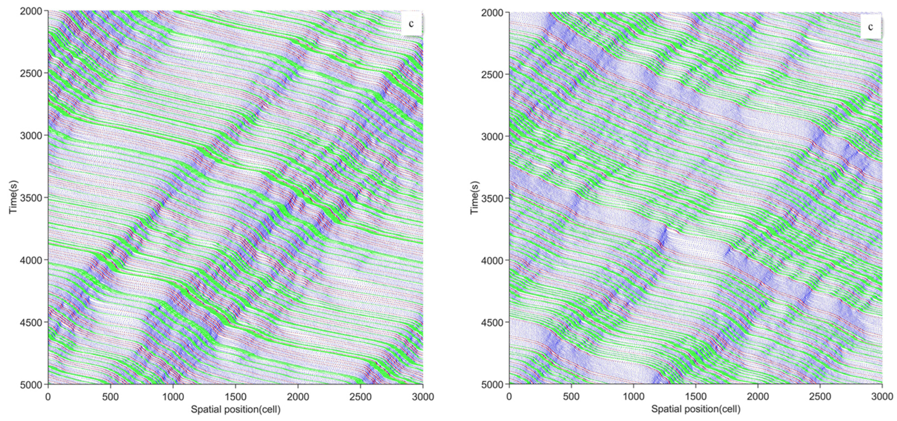
In this section, from the perspective of the maximum vehicle platoon length, the influence of it on the degree of road congestion is observed. The driving trajectory of the simulation process is illustrated in the spatio-temporal diagrams of stable traffic flow. The medium-density traffic flow with 60% CAV permeability and 60 pcu/km (all density values in this paper refer to each single lane) is taken as an example, as shown in Figure 1. This represents two lanes with three different maximum platoon lengths. Here, the white cell represents the road space not occupied by vehicles; the blue cell represents the HDV; the red cell is the CAV that does not participate in any formation because of not meeting the conditions for platooning; and the green cell is the vehicles in a platoon formed of CAVs according to the set parameters and the platoon evolution rules.

The spatio-temporal diagrams show that in medium density traffic flow with CAV permeability reaching 60%, extremely serious congestion will not easily occur on the whole.

The average travel times of each vehicle under the three maximum platoon lengths are not very different. Comparing the congestion conditions under the three maximum platoon length settings, we see that the maximum platoon length of two is relatively significant, while the maximum platoon lengths of five and eight can be seen to improve, as is mainly reflected in the smaller range of congestion and faster dissipation speed. However, when the maximum platoon length is eight, although the congestion dissipates quickly, subtle speed mutations also occur more frequently. From the spatio-temporal diagrams, we can see that a large number of vehicles frequently alternate acceleration and deceleration in almost all covered time steps, and the traffic flow cannot travel at a speed close to free flow over long distances. In contrast, when the maximum platoon length is five, the traffic flow congestion does not dissipate as quickly as when the maximum platoon length is eight, but the reverse wave of the congestion phenomenon is transmitted more quickly upstream, and when the vehicle pulls out of the congested section, it can travel in the free flow state over a longer distance.

3.3. Influence of Maximum Platoon Length on Average Speed of Traffic Flow

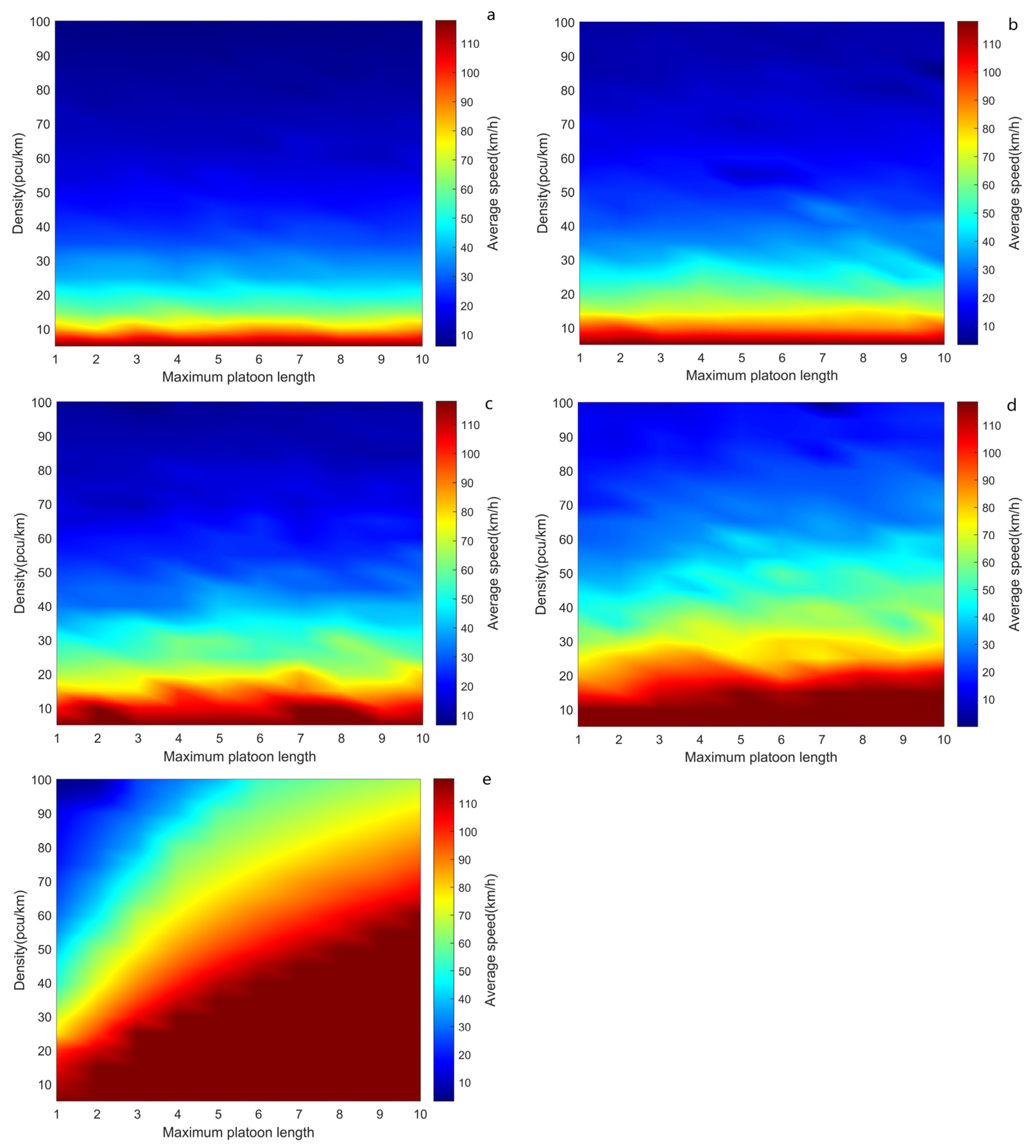
We take the average of the density data for the two lanes, based on multiple CAV permeability and speed–density fundamental heat maps for maximum platoon lengths. Figure 2 presents velocity–density fundamental diagrams, expressed in the form of heat maps (hereafter, fundamental diagram-heat maps) with five different CAV permeabilities. It can be seen from Figure 2 that the increase in CAV permeability can effectively ensure the relatively high speed of vehicles when the road is subjected to higher-density traffic flow. With the decrease in CAV permeability, the average velocity decreases faster with the increase in density. And the density corresponding to the same average velocity moves horizontally to a higher value in the fundamental diagram-heat maps; that is, it moves to the high-density region with the increase in CAV permeability. At the same time, when CAV permeability is low (especially 20%), a change in maximum platoon length has little effect on the traffic flow at the corresponding density. When the CAV permeability is 40%, there is basically no effect, only some slight changes caused by random disturbances, which are not enough to reach meaningful conclusions. When the CAV permeability reaches 60%, the influence of the maximum platoon length on the average speed at the same density can be effectively reflected in the medium- and low-speed parts below 60 km/h, that is, with the increase in the maximum platoon length, the average speed at the same density increases. This phenomenon is further reflected with the CAV permeability of 80%. The influence is relatively more significant, and we see a tendency towards a speed of about 60 km/h. When CAV permeability is 100%, that is, in homogeneous traffic flow with all-CAV participation, the above rules are most clearly reflected. As the maximum platoon length increases, higher densities can persist and the speed limit can be almost maintained, and the critical density at which the average speed collapses shifts to the right. For example, when the maximum platoon length is 10 vehicles, all vehicles can still drive at the maximum speed limit on average in a medium–high-density traffic flow of 70 pcu/km. Moreover, the increase in the maximum platoon length can significantly increase the average speed in each density interval, and this regularity is very stable, but there is a significant amplitude span between the same law and the heterogeneous traffic flow. It is shown that the maximum platoon length has a significant effect on the average speed of the whole connected automated traffic flow.

3.4. Study on the Impact of Maximum Platoon Length on the Road Capacity

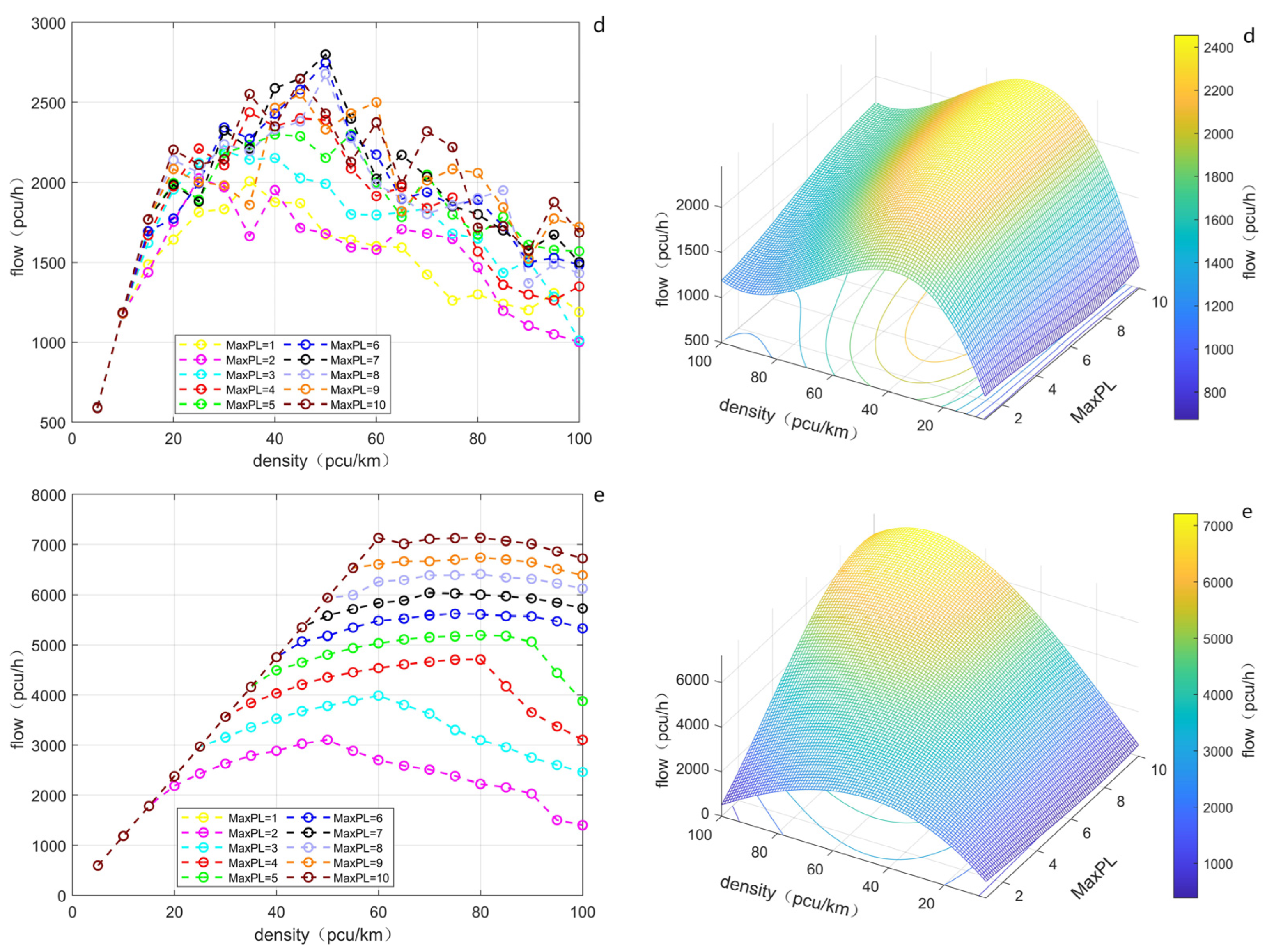
Under the same simulation conditions, this study has further explored the influence of the maximum platoon length on road capacity. The flow–density diagrams for five different CAV permeabilities and the 3D diagrams generated by the fitting results are illustrated in Figure 3.

From the perspective of the maximum platoon length (“maxPL” in all Figures below), the higher the CAV permeability, the greater the impact of the maximum platoon length setting on the flow–density diagrams. Especially at medium–high density, the disparity between the flows corresponding to different maximum platoon lengths at the same density became bigger, indicating that the sensitivity of traffic flow to the parameters of the maximum platoon length increases. Up until the CAV permeability of 100%, the maximum length of the platoon can have a significant impact on the traffic flow at the same density.

On the whole, when the CAV permeability is below 50%, only a small numbers of CAVs are driving on the road, and according to the evolution rules, there will not be a large number of platoons, so the flow difference in heterogeneous traffic flow with different maximum platoon lengths is not large. When the CAV permeability is more than 50%, there will be more CAVs participating in traffic on the road, and the number of CAV platoons formed will gradually increase, with more opportunities to form longer platoons, which is the reason for the increased sensitivity of the maximum platoon length parameter. Furthermore, the inclusion of CAVs and the participation of the platoon will improve the heterogeneous traffic flow capacity, which often reaches its most significant state at the critical density. In addition, when the traffic flow remains mixed, the influence of the maximum platoon length shows the obvious characteristic of being easily disturbed by random factors, and this characteristic gradually decreases with the increase in CAV permeability.

When the CAV permeability is 20%, the maximum platoon length on the whole has little influence on the heterogeneous traffic flow, because the participation of CAV in the traffic flow is not high and the influence is insufficient. When CAV permeability reaches 40%, the influence of the maximum platoon length on the expressway heterogeneous traffic flow initially appears. This shows that when the maximum platoon length is large, the overall traffic flow in each density interval is slightly higher. However, it is worth noticing that when the medium density traffic flow is near 40 pcu/km, the maximum platoon length is longer than seven vehicles, and the traffic flow shows a downward trend. When CAV permeability reaches 60%, the influence of maximum platoon length is further elaborated. The region in which the maximum platoon length is low starts to move away from the peak flow of the whole surface, and the peak area moves to the region where the maximum platoon length is greater, but the growth rate of the flow at an equal density slows down with the increase in the maximum platoon length. When CAV permeability reaches 80%, there are significant differences in traffic flow between different maximum platoon lengths in medium–high-density heterogeneous traffic flows. In the process of increasing the maximum platoon length from two to six vehicles, the traffic flow at an equal density is increased significantly, and this phenomenon is still typical in the medium–high-density region. When the traffic flow becomes homogeneous with full CAV participation, within the range of vehicle platoon lengths selected in this study, the traffic flow increases monotonically with the increase in the maximum vehicle platoon length, and the increase amplitude is extremely significant; the traffic flow not only moves in the direction of the maximum vehicle platoon length, but also moves in the direction of higher density. This can suggest that the increase in the maximum platoon length allows the traffic flow to tolerate higher densities and maintain a relatively considerable road capacity, but it also shows that this capacity is capped, because the inflection point occurs near the density of 80 pcu/km. In addition, the influence of parameter changes on the flow still shows very stable regularity at this time, which shows that the connected automated traffic flow will also have stronger robustness resulting from the system.

Figure 4 illustrates a comparison of multiple three-dimensional surfaces combined in the same coordinate system under conditions of different and heterogeneous traffic flow permeabilities. The influences of different CAV permeabilities show diversities and regularity. The higher the CAV permeability, the more obvious the influence of the maximum platoon length on the traffic flow, and also the more significant the parameter characteristics, which suggests that the longer the maximum platoon length, the greater the traffic flow under the same conditions.

4. Study on the Influence of Maximum Platoon Length on the Stability and Safety of Traffic Flow

4.1. Stability Evaluation of Heterogeneous Traffic Flow

Standard Deviation (SD) is a commonly used method to measure the degree of dispersion of a data set in probability statistics. In heterogeneous traffic flow, the difference in vehicle speeds can reflect the smoothness of traffic flow, and the stability is reflected in changes in cars’ speeds. Therefore, the speed SD is adopted as an evaluation index of heterogeneous traffic flow stability in this study, and its calculation formula is as follows [62]:

$$SD=\sqrt{\frac{{\displaystyle \sum _{n=1}^N{(v_n-\overline{v})}^2}}{N-1}}$$

(17)

where v_n is the speed of vehicle n within the simulation time step; $\overline{v}$ is the average speed of all vehicles within the simulation time step; N is the number of simulated vehicles.

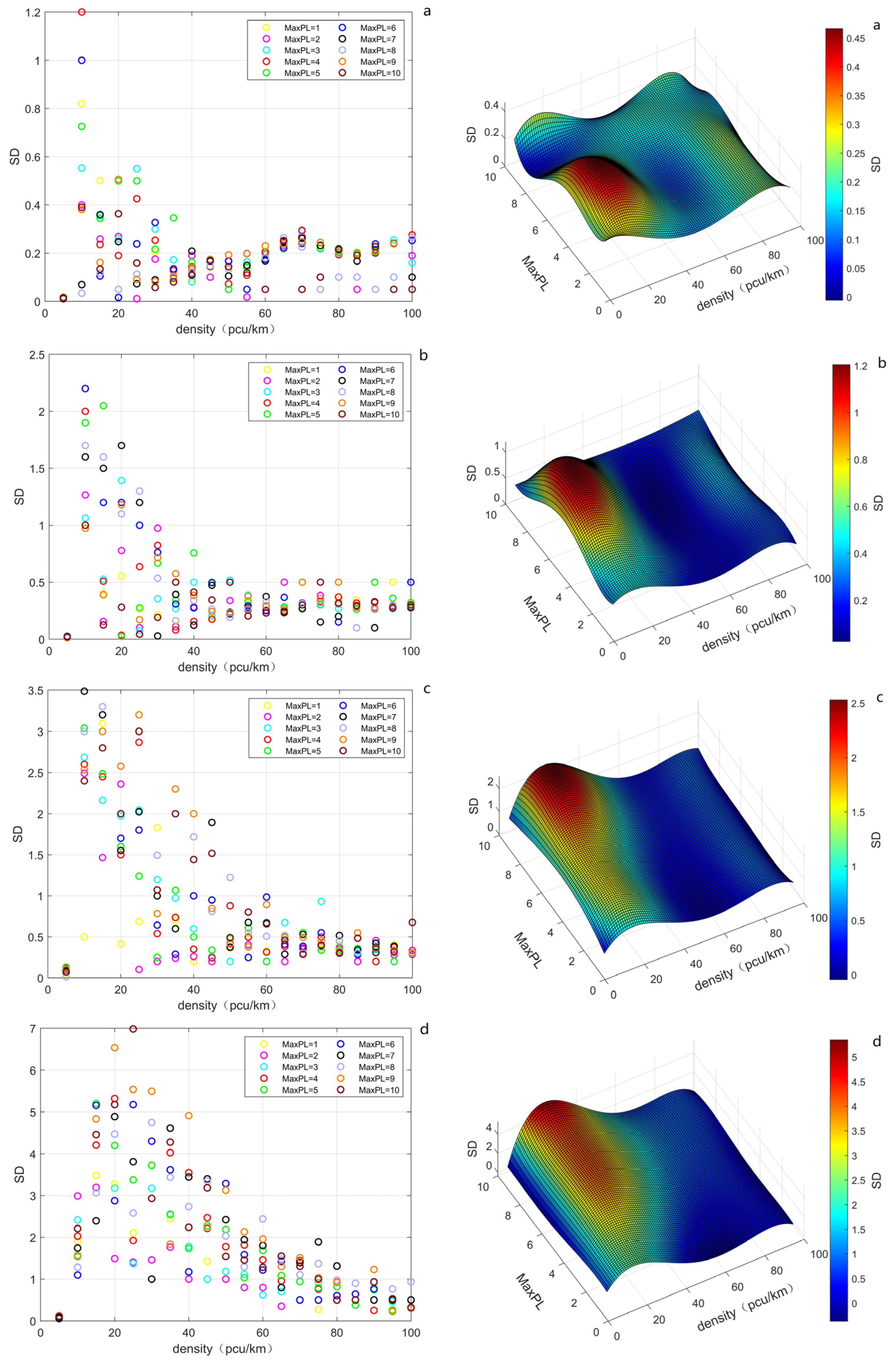
The magnitude of the sample SD can be used to describe the degree of aggregation of the sample data. When the speed SD is small, it means that the speed difference between vehicles in heterogeneous traffic flow with CAV participation is small, and the flow is relatively stable. On the basis of the experimental data from the previous experiment, the changes in speed SD for different maximum platoon lengths were calculated. The SD data of density–maximum platoon length with five different CAV permeabilities and the 3D diagrams generated from their fitting results are illustrated in Figure 5.

When the CAV permeability is 20%, the effect of the maximum platoon length on SD is mainly reflected in the low-density area, and the SD is higher when the maximum platoon length is two to five vehicles. The maximum platoon length has no obvious effect on SD when the density reaches more than 40 pcu/km. When CAV permeability is 40%, it can be seen from the peak position of the entire surface that the region whereat the maximum platoon length has a significant effect on SD is still in the low-density region, but moves towards a higher maximum platoon length, concentrated between four and eight. When the CAV permeability is 60%, the influence of the maximum platoon length on SD is further expanded, and the area of significant influence is still in the low-density region, moving towards the region of greater maximum platoon length, concentrated between 6 and 10. On the other surface, the high SD value range begins to shrink in the region with a lower maximum platoon length. When the CAV permeability reaches 80%, the CAV plays a leading role in traffic flow. The range over which the maximum platoon length has a significant effect on SD is obviously expanded, and the covered area is extended to medium density. When CAV permeability reaches 100%, the range of influence of maximum platoon length on SD expands significantly, and the peak value not only moves in the direction of higher maximum platoon length, but also moves in the direction of high density, reaching a medium-density area near 40–60 pcu/km, and it then falls again with the continuous increase in density.

Through the above analysis, it can be observed that, under the same CAV permeability conditions, SD changes significantly only in the direction of the maximum platoon length in the low-density region, and the effect is small in the medium–high-density region. In the process of increasing CAV permeability, the influence range of maximum platoon length on SD gradually expands, and the peak position moves regularly. In this case, this study argues that the higher the CAV permeability, the stronger its dominance in traffic flow, the more obvious the speed advantage of formation driving, and the greater the difference compared with HDVs. However, in the vast majority of cases, this dynamic effect varies only at low densities, where traffic flow is strongly affected by the randomness of speed differences. Therefore, it cannot be concluded that “CAVs affect the stability of traffic flow”.

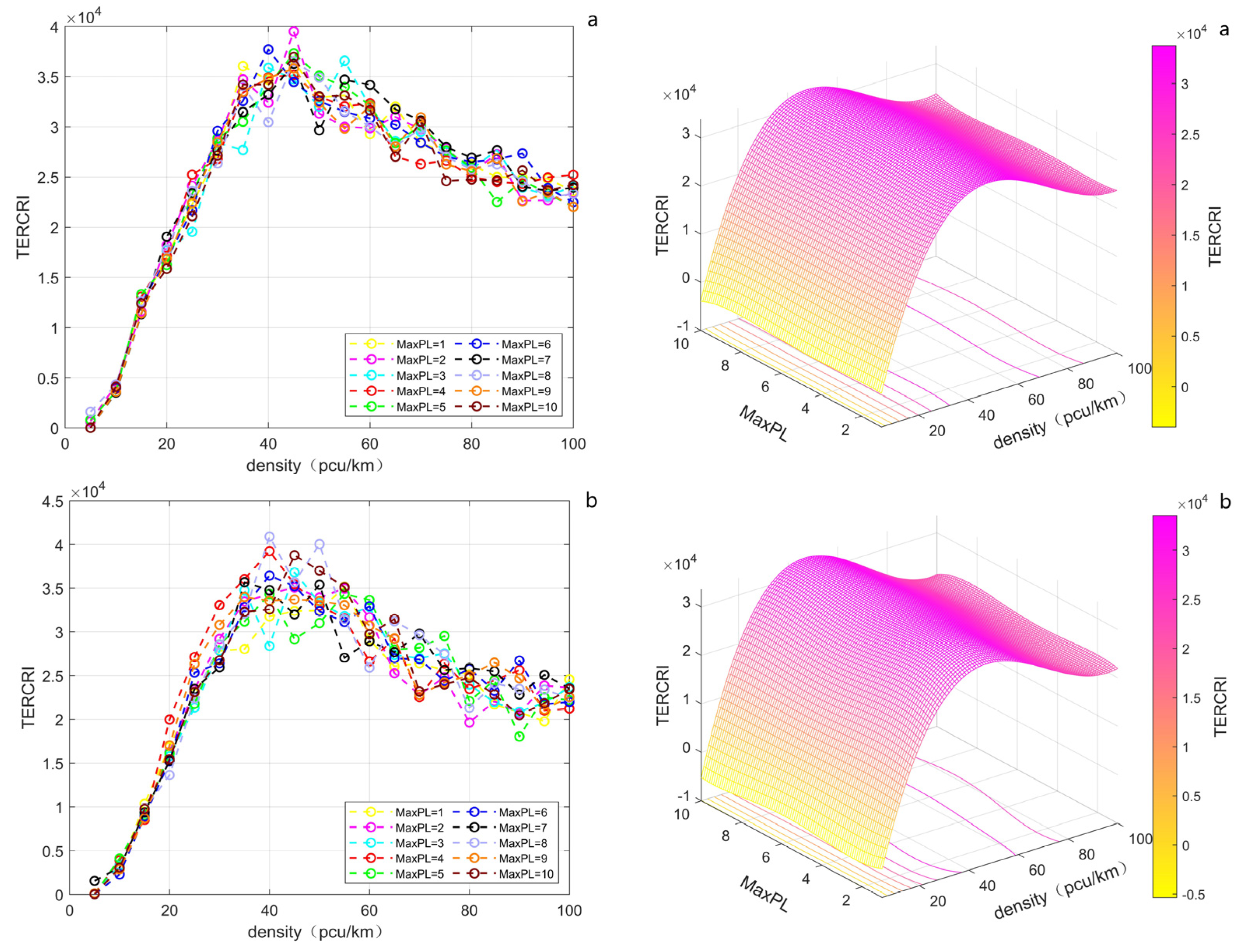
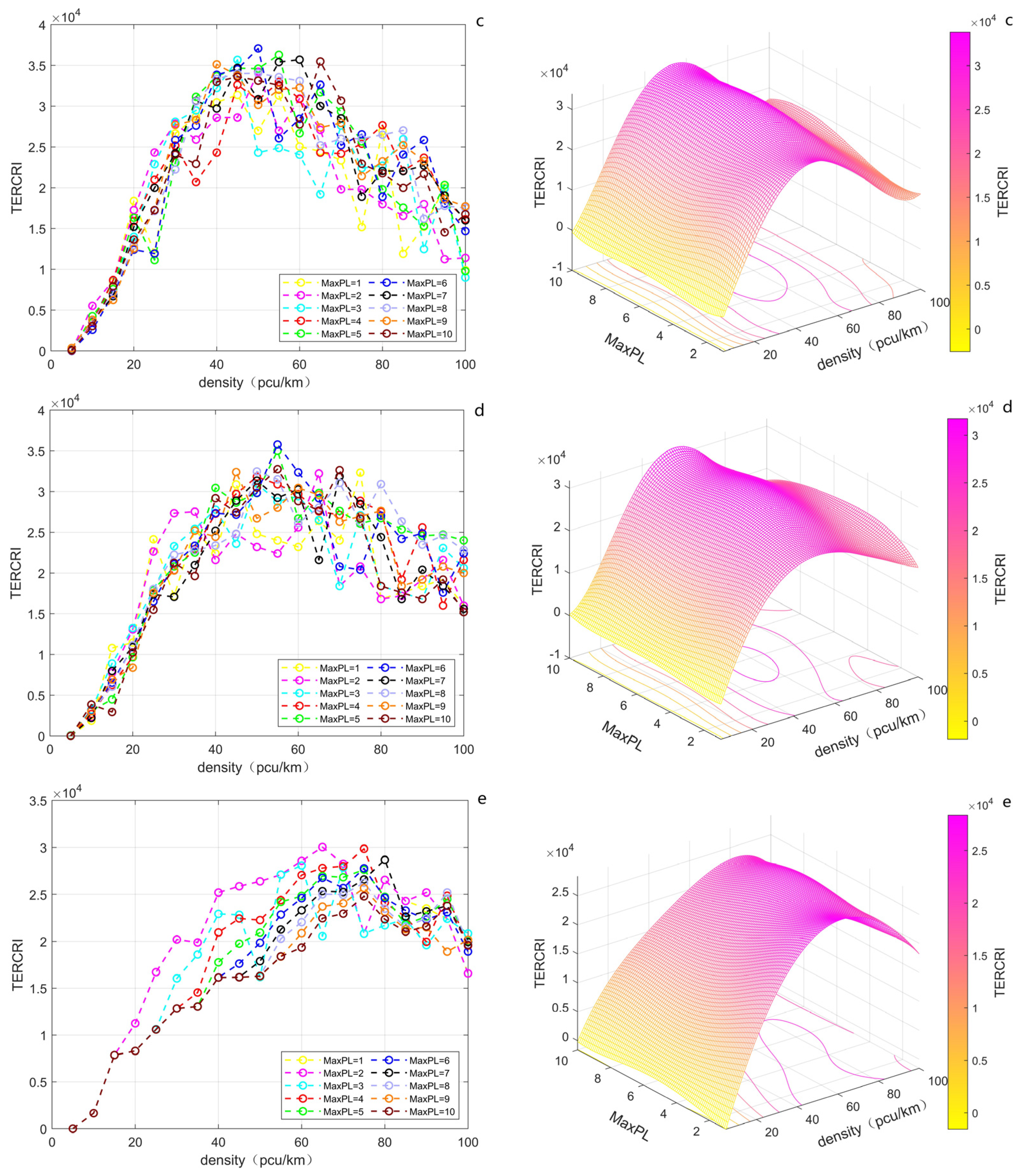
4.2. Safety Evaluation of Heterogeneous Traffic Flow

On the expressway, vehicles usually travel at a high speed. Therefore, not maintaining a sufficient safety distance between the front and rear vehicles is the main cause of rear-end collisions, which are the most common type of expressway traffic accidents. The Time-Exposed Rear-End Collision Risk Index (TERCRI) is often used to indicate the risk of a rear-end collision due to the speed of the vehicle in front of the car slowing down too quickly for the rear car to brake, resulting in rear-end collisions because of the insufficiently safe distance between the front and rear cars. The formula is as follows [63]:

$$S{D}_L=v_{n+1}\cdot h+\frac{v_{n+1}^2}{2a_{n+1}}+L$$

(18)

$$S{D}_F=v_n{t}_{PRT}+\frac{v_n^2}{2a_n}$$

(19)

If SD_L < SD_F, then the braking distance of the following vehicle is greater than the braking distance of the front vehicle, resulting in an insufficient safety distance and rear-end collisions.

$$TERCRI(t)={\displaystyle \sum _{n=1}^N{\displaystyle \sum _{t=1}^{T}RCR{I}_n(t)\times \Delta t}}$$

(20)

Therein:

$$RCR{I}_n(t)=\left\{\begin{array}{c}1, S{D}_F>S{D}_L\\ 0, S{D}_F\le S{D}_L\end{array}\right\}$$

(21)

where SD_L and SD_F are, respectively, the braking distances of the preceding vehicle and the rear vehicle; L is the vehicle length; h is the time headway; t_PRT is the perceived response time of following vehicle, the values of which are as shown in Table 1; N is the number of simulated vehicles; T is the simulation duration.

In order to further explore the impact of platoon length on the safety of heterogeneous traffic flow on the expressway, this study calculated, and constructed curve fittings for, the changes in TERCRI with different maximum platoon lengths on the basis of previous experiments. Figure 6 shows the density with five different CAV permeabilities, as well as the TERCRI data of maximum platoon length, and the 3D diagrams generated according to their fitting results.

In general, the TERCRI value increases first and then falls with the increase in density, and the peak position is about 40–60 pcu/km. Obviously, the reduced speed at which vehicles are forced to travel when there is high density plays a positive role in the safety of traffic flow. When the CAV permeability is 20%, the TERCRI at a density of 100 pcu/km is reduced about 30% compared to the peak. At the same time, CAVs are less involved in the traffic, so the influence of the maximum platoon length on TERCRI at this time is not detectable in the full density range. When CAV permeability reaches 40%, relative to the results for 20%, the TERCRI does not change with the density as a whole, and there is no significant change along the direction of the maximum platoon length. Only under the medium–high-density conditions of 60–80 pcu/km is the TERCRI slightly higher when the maximum platoon length is larger. When CAV permeability reaches 60%, the TERCRI decreases overall, by about 10% at the peak location and by about 35% at the density of 100 pcu/km. Secondly, the peak location begins to show a slight trend towards higher density. Third, the degree of data affected by random factors is further increased, and the interval is extended into the region of low density. When the CAV permeability reaches 80%, the inflection point moves into the range of 50–60 pcu/km, and the overall value and peak value are further decreased, while the decline is not obvious at the density of 100 pcu/km. The degree of data affected by random factors is further increased, and this is more reflected in the medium–high-density region than in the low-density region. In addition, the rule that TERCRI increases with the increase in the maximum platoon length at medium–high density further appears, especially when the density is between 40 and 60 pcu/km, at which point TERCRI increases monotonically in the direction of the change with 2–10 vehicles until reaching the maximum platoon length, indicating that the setting of the maximum platoon length can be effectively pursued. When the CAV permeability reaches 100%, the inflection point moves into the 60–70 pcu/km range in the density direction, and the overall value decreases further, with a peak decline of about 15%. The extent of data affected by random factors is still obvious. The medium- and low-density parts show obvious characteristics of being affected by the maximum platoon length. At this point, in the region of maximum platoon length, the smaller the maximum platoon length is under the condition of equal density, the higher the TERCRI will be, especially regarding the medium- and low-density parts. So, when the traffic flow is homogeneous and represented exclusively by CAVs, it is better to set a higher maximum platoon length. After the traffic flow has completely eliminated the interference of HDVs, the presence of CAVs can actually improve the safety of traffic flow. According to the above analysis, TERCRI changes little in the direction of maximum platoon length on the whole, indicating that the maximum platoon length has no strong influence on traffic flow safety from the perspective of TERCRI. When CAV permeability is low, the impact of the maximum platoon length on safety is negligible. When CAV permeability exceeds 1/2, the impact of the maximum platoon length can be seen to some degree in the medium–high-density region. We believe that because the traffic flow is heterogeneous, the presence of a few HDVs participating in the traffic flow will cause interference for CAVs and their platoon formation. The evidence is that when the traffic flow is 100% CAV, longer maximum platoon lengths under the same density conditions lead to greater safety.

According to the above analysis, TERCRI shows little change in the region of maximum platoon length on the whole, indicating that the maximum platoon length has no strong influence on traffic flow safety from the perspective of TERCRI. When CAV permeability is low, the impact of the maximum platoon length on safety is negligible. With a CAV permeability exceeding 1/2, a slight impact of the maximum platoon length can be seen in the medium–high-density region.

5. Summary and Conclusions

This study on the effects of the maximum platoon length on the characteristics of fundamental diagrams of heterogeneous traffic flow shows that, when the maximum platoon length is five, the vehicles can drive over a long distance in the state of free flow on non-congested road sections, and in medium–high-density traffic flow with a certain degree of CAV permeability, the average speeds of the formation vehicles in the traffic flow change more regularly, the speeds of non-formation vehicles are more stable, and the average speed overall reaches optimality. When CAV permeability is moderate, the average speed increases with the increase in the maximum platoon length, but this improvement begins to slow down when the maximum platoon length increases to five vehicles. When CAV permeability reaches a higher level, a longer maximum platoon length leads to a greater average speed with equal density, and the degree increases as the CAV permeability approaches 100%. The characteristics of traffic flow are consistent with those of heterogeneous traffic flow when the traffic flow becomes fully connected and autonomous, but there are still great differences in the change amplitudes of traffic flow characteristics.

Our study on the effects of maximum platoon length on the stability and safety of heterogeneous traffic flow shows that the maximum platoon length has a certain impact on the stability and safety of heterogeneous traffic flow. With the increase in CAV permeability, the SD value is increased and the TERCRI value is decreased. When the CAV permeability is high, the SD peak value, which describes stability, moves in the direction of maximum platoon length. When the CAV permeability reaches 100%, the SD peak value diffuses in the direction of medium–high density. Under the condition of medium–high density, the increases in CAV permeability and maximum platoon length will not cause the traffic flow to lose stability. A high maximum platoon length will affect the safety of heterogeneous traffic flow to a small extent, but it can be ignored when the CAV permeability is low. This effect gradually appears with the increase in CAV permeability, and will be lifted automatically when the CAV permeability reaches 100%.

In conclusion, if the CAV permeability does not reach a high level, combined with the current situation according to which China’s expressways often feature medium–high-density traffic flow, considering the comprehensive influence of platoon length on the characteristics of traffic flow and the collective interests of traffic, the maximum platoon length should be set a threshold value, which should be agreed at around five vehicles. When the CAV permeability is close to 100%, the threshold value of maximum platoon length can be less strictly limited. This conclusion is mutually supported by other high-level similar studies performed in the domestic environment and overseas [60,62]. At the same time, it is a novel finding that the effect exerted by the maximum platoon length on its properties, whether in terms of fundamental diagrams, stability or safety, when penetration reached 100% produced a significant change in magnitude of the type never seen before. The national standards of The CAV Technology Roadmap 2.0 and The Automotive Driving Automation Classification propose that domestic level 2 and 3 CAVs will reach a prevalence of 50% in 2025 and 70% in 2030. According to the development plans for CAVs in relation to the recommendation standards of different countries, it can be predicted that CAVs will not reach a very high level of permeability. Therefore, combined with the research conclusions of this paper, before 2030, China’ s threshold value for the maximum platoon length of CAVs driving on the road should still be restricted to about four to six cars. In the longer term, discerning the optimal platoon length will represent a dynamic process that needs to be adjusted to adapt to different traffic environments.

This paper studies the effects of maximum platoon length on heterogeneous traffic flow characteristics on multi-lane expressways, and has obtained some interesting results. In view of the limited research level and scope, the following issues should be further explored.

First of all, the difference between different intelligence levels of CAVs will definitely bring more complex and changeable characteristics to heterogeneous traffic flow. The two kinds of “artificial intelligence” will eventually fail to meet the research needs of greater precision and detail. The complex state of coexistence of CAVs with different intelligence levels should be introduced into the modeling process of heterogeneous traffic flow characteristics. Secondly, according to the findings herein, when CAV permeability is close to 100%, the setting of the maximum platoon length may not be limited to less than 10 vehicles. The capacity for influence and the general law of the maximum platoon length may undergo a qualitative change when the CAV permeability reaches a high level. This qualitative change is likely to make it necessary to extend the study of maximum platoon length to more than 10 vehicles. In addition, we can also further refine and optimize this model and other corresponding ones through the following methods: distinguishing the differences in acceleration characteristics according to the different inherent dynamic performances of vehicles; focusing on bottlenecks, in particular on-ramp/weaving merging and other more complex expressway environments; setting up special lanes for CAVs to improve road utilization, and considering the communication burden of longer platoons as leading to data transmission delays. As these research conditions could not provide the authors with a large amount of reliable experimental data, some further discussions and experiments will have to be undertaken in follow-up research. The authors will continue to work on verifying the correlation between the model and reality in future studies.