
Analytical Explicit Formulas of Average Run Length of Homogenously Weighted Moving Average Control Chart Based on a MAX Process

Abstract
:1. Introduction
2. Materials and Methods
2.1. Control Charts
2.1.1. Homogenously Weighted Moving Average (HWMA) Control Chart
2.1.2. Cumulative Sum (CUSUM) Control Chart
2.2. Characteristics of Average Run Length
3. Average Run Length for MAX(q,r) Process
3.1. The Explicit Formula Method
3.2. Numerical Integral Equation Method
3.3. Existence and Uniqueness of ARL
4. Numerical Results
- i
- Determine the exponential white noise and smoothing parameters for the in-control process.
- ii
- Determine the initial values for the MAX(q,r) process and the HWMA statistic.
- iii
- Select acceptable values for ARL0 and the shift sizes
- iv
- Compute the upper control limit (b) that yields the desired ARL for the control process using (3).
- i
- Compute ARL0 using (3) when given the upper control limit (b) from Step 1.
- ii
- Approximate the value of ARL0 via the NIE method by using (5).
- iii
- If necessary, change the value of b according to the desired ARL0 value.
- i
- Compute ARL1 for various shift sizes and by using (4) and the value of b from Step 1.
- ii
- Approximate ARL1 via the NIE method by using (5).
- iii
- Compare the ARL values obtained using the explicit formulas and NIE methods.
5. Practical Applications with Real Data
- To estimate parameters from interesting data such as stock price, which must include a MAX model.
- To estimate the parameter of exponentially distributed residuals.
- Using the parameter values from 1 and 2, determine the ARL value in Equations (3) and (4).
- To compare the performance using the ARL value calculated from 3 and other control charts.
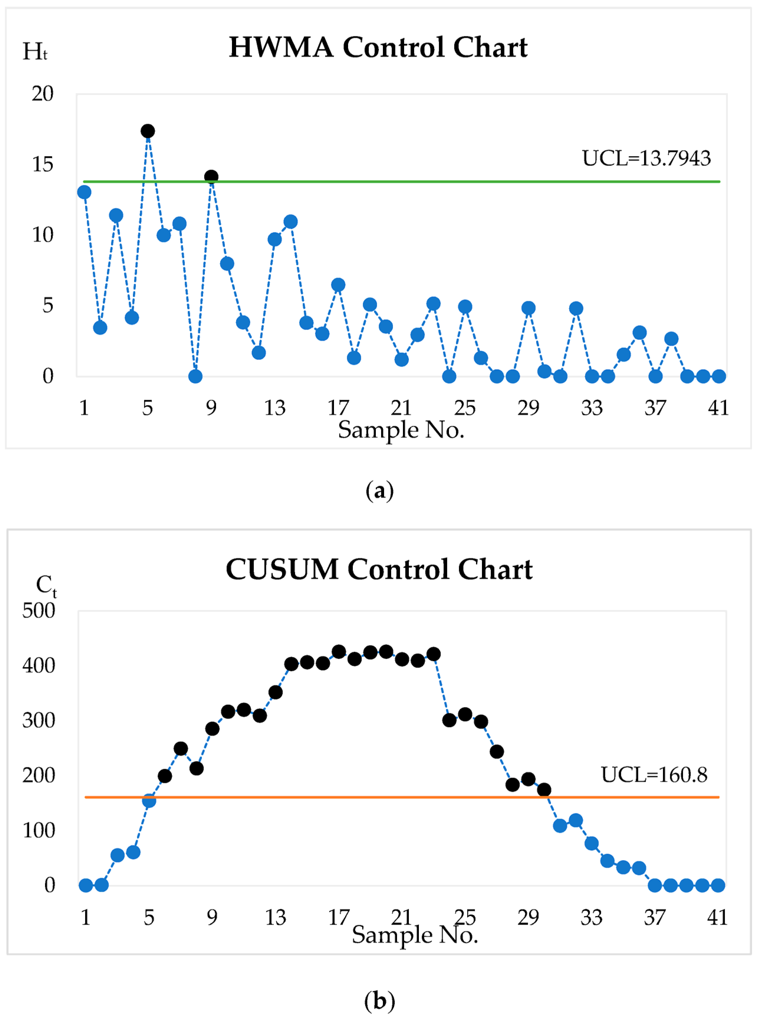
- To detect changes in the process mean, determine the UCL value using the equation in (3) and use actual data to compute control chart statistics before plotting the control chart statistics on a graph.
6. Discussion and Conclusions
Author Contributions
Funding
Data Availability Statement
Acknowledgments
Conflicts of Interest
Appendix A
Appendix B
References
- Page, E.S. Continuous inspection schemes. Biometrika 1954, 41, 100–115. [Google Scholar] [CrossRef]
- Roberts, S. Control chart tests based on geometric moving averages. Technometrics 1959, 42, 239–250. [Google Scholar] [CrossRef]
- Abbas, N. Homogeneously weighted moving average control chart with an application in substrate manufacturing process. Comput. Ind. Eng. 2018, 20, 460–470. [Google Scholar] [CrossRef]
- Knoth, S.; Tercero-Gómez, V.G.; Khakifirooz, M.; Woodall, W.H. The impracticality of homogeneously weighted moving average and progressive mean control chart approaches. Qual. Reliab. Eng. Int. 2021, 37, 3779–3794. [Google Scholar] [CrossRef]
- Riaz, M.; Ahmad, S.; Mahmood, T.; Abbas, N. On Reassessment of the HWMA Chart for Process Monitoring Muhammad. Processes 2022, 10, 1129. [Google Scholar] [CrossRef]
- Lucic, M.; Xydis, G. Performance of the autoregressive integrated moving average model with exogenous variables statistical model on the intraday market for the Denmark-West bidding area. Energy Environ. 2023, 2023, 0958305X231199154. [Google Scholar] [CrossRef]
- Phengsalae, Y.; Areepong, Y.; Sukparungsee, S. An Approximation of ARL for Poisson GWMA using Markov Chain Approach. Thail. Stat. 2015, 13, 111–124. [Google Scholar]
- Riaz, M.; Zaman, B.; Mehmood, R.; Abbas, N.; Abujiya, M. Advanced multivariate cumulative sum control charts based on principal component method with application. Qual. Reliab. Eng. Int. 2021, 37, 2760–2789. [Google Scholar] [CrossRef]
- Bualuang, D.; Peerajit, W. Performance of the CUSUM Control Chart using Approximation to ARL for Long-Memory Fractionally Integrated Autoregressive Process with Exogenous Variable. Appl. Sci. Eng. Prog. 2023, 16, 5917. [Google Scholar] [CrossRef]
- Chananet, C.; Phanyaem, S. Improving CUSUM Control Chart for Monitoring a Change in Processes Based on Seasonal ARX Model. IAENG Int. J. Appl. Math. 2022, 52, IJAM_52_3_08. [Google Scholar]
- Phanyaem, S. The integral equation approach for solving the average run length of EWMA procedure for autocorrelated process. Thail Stat. 2021, 19, 627–641. [Google Scholar]
- Supharakonsakun, Y. Comparing the effectiveness of statistical control charts for monitoring a change in process mean. Eng. Lett. 2021, 29, 1108–1114. [Google Scholar]
- Petcharat, K. The Effectiveness of CUSUM Control Chart for Trend Stationary Seasonal Autocorrelated Data. Thail Stat. 2022, 20, 475–488. [Google Scholar]
- Peerajit, W. Developing Average Run Length for Monitoring Changes in the Mean on the Presence of Long Memory under Seasonal Fractionally Integrated MAX Model. Math. Stat. 2023, 11, 34–50. [Google Scholar] [CrossRef]
- Petcharat, K. Designing the performance of EWMA control chart for seasonal moving average process with exogenous variables. IAENG Int. J. Appl. Math. 2023, 53, 1–9. [Google Scholar]
- Suriyakat, W.; Petcharat, K. Exact Run Length Computation on EWMA Control Chart for Stationary Moving Average Process with Exogenous Variables. Math. Stat. 2022, 10, 624–635. [Google Scholar] [CrossRef]
- Crowder, S.V. A simple method for studying run length distributions of exponentially weighted moving average charts. Technometrics 1987, 29, 401–407. [Google Scholar]
- Champ, C.W.; Rigdon, S.E. A comparison of the Markov chain and the integral equation approaches for evaluating the run length distribution of quality control charts. Commun. Stat. Simul. Comput. 1991, 20, 191–204. [Google Scholar] [CrossRef]
- Srivastava, M.S.; Wu, Y. Comparison of EWMA, CUSUM and Shiryayev-Roberts procedure for detecting a shift in the mean. Ann. Stat. 1993, 21, 645–670. [Google Scholar] [CrossRef]
- Srivastava, M.S.; Wu, Y. Evaluation of optimum weights and average run lengths in EWMA control schemes. Commun. Stat. Theory Methods 1997, 26, 1253–1267. [Google Scholar] [CrossRef]
- Phanyaem, S. Explicit Formulas and Numerical Integral Equation of ARL for SARX(P,r)L model based on CUSUM Chart. Math. Stat. 2022, 10, 88–99. [Google Scholar] [CrossRef]
- Sofonea, M.; Han, W.; Shillor, M. Analysis and Approximation of Contact Problems with Adhesion or Damage; Chapman & Hall/CRC: New York, NY, USA, 2005. [Google Scholar]
- Tang, A.; Castagliola, P.; Sun, J.; Hu, X. Optimal design of the adaptive EWMA chart for the mean based on median run length and expected median run length. Qual. Technol. Quant. Manag. 2018, 16, 439–458. [Google Scholar] [CrossRef]
- Fonseca, A.; Ferreira, P.H.; Nascimento, D.C.; Fiaccone, R.; Correa, C.U.; Piña, A.G.; Louzada, F. Water Particles Monitoring in the Atacama Desert: SPC approach Based on proportional data. Axioms 2021, 10, 154. [Google Scholar] [CrossRef]

| Models | Coefficients | |||||||||
|---|---|---|---|---|---|---|---|---|---|---|
| = 0.1 | = 0.2 | = 0.3 | ||||||||
| MAX(1,1) | 1 | 0.1 | 0.2 | 0.0014638 | 0.06065 | 0.10252 | ||||
| MAX(1,2) | 1 | 0.1 | 0.2 | 0.3 | 0.0010800 | 0.04440 | 0.074865 | |||
| MAX(1,3) | 1 | 0.1 | 0.2 | 0.3 | 0.4 | 0.0007230 | 0.02944 | 0.049523 | ||
| MAX(2,1) | 1 | 0.1 | 0.2 | 0.2 | 0.0017900 | 0.07483 | 0.12679 | |||
| MAX(2,2) | 1 | 0.1 | 0.2 | 0.2 | 0.3 | 0.0013220 | 0.05464 | 0.09227 | ||
| MAX(2,3) | 1 | 0.1 | 0.2 | 0.2 | 0.3 | 0.4 | 0.0008850 | 0.03614 | 0.060845 | |
| MAX(3,1) | 1 | 0.1 | 0.2 | 0.3 | 0.2 | 0.0024200 | 0.10300 | 0.17547 | ||
| MAX(3,2) | 1 | 0.1 | 0.2 | 0.3 | 0.2 | 0.3 | 0.0017900 | 0.07483 | 0.12679 | |
| MAX(3,3) | 1 | 0.1 | 0.2 | 0.3 | 0.2 | 0.3 | 0.4 | 0.0011950 | 0.04925 | 0.08309 |
| 0.1 b = 0.001195 | ARC(%) | 0.2 b = 0.04925 | ARC(%) | ||||
| Explicit Formula | NIE | Explicit Formula | NIE | ||||
| −0.1 | 0 | 370.3770885 | 370.377 | 2.390 × 10⁻⁵ | 370.5593435 | 370.559 | 9.270 × 10⁻⁵ |
| 0.001 | 366.1943273 | 366.194 | 8.938 × 10⁻⁵ | 362.1715955 | 362.172 | 0.00011677 | |
| 0.003 | 357.9938367 | 357.994 | 4.560 × 10⁻⁵ | 346.3219822 | 346.322 | 5.133 × 10⁻⁶ | |
| 0.005 | 350.0079350 | 350.008 | 1.858 × 10⁻⁵ | 331.600544 | 331.60 | 1.641 × 10⁻⁵ | |
| 0.01 | 330.9408108 | 330.941 | 5.718 × 10⁻⁵ | 299.0211502 | 299.021 | 5.023 × 10⁻⁵ | |
| 0.03 | 265.9258522 | 265.926 | 5.558 × 10⁻⁵ | 209.3451951 | 209.345 | 9.320 × 10⁻⁵ | |
| 0.05 | 215.4434020 | 215.443 | 0.00018659 | 156.1001736 | 156.100 | 0.00011124 | |
| 0.1 | 131.5709136 | 131.571 | 6.564 × 10⁻⁵ | 87.70901617 | 87.7090 | 1.844 × 10⁻⁵ | |
| 0.3 | 26.90378287 | 26.9038 | 6.368 × 10⁻⁵ | 21.56693573 | 21.5669 | 0.00016565 | |
| 0.5 | 8.762648041 | 8.76265 | 2.236 × 10⁻⁵ | 9.417738995 | 9.41774 | 1.067 × 10⁻⁵ | |
| 1.0 | 2.039095587 | 2.03910 | 0.00021643 | 3.137729377 | 3.13773 | 1.984 × 10⁻⁵ | |
| 3.0 | 1.039333882 | 1.03933 | 0.00037350 | 1.245405834 | 1.24541 | 0.00033454 | |
| 5.0 | 1.011101932 | 1.01110 | 0.00019107 | 1.102469633 | 1.10247 | 3.333 × 10⁻⁵ | |
| 0.1 b = 0.001463 | ARC(%) | 0.2 b = 0.06065 | ARC(%) | ||||
| Explicit Formula | NIE | Explicit Formula | NIE | ||||
| 0.1 | 0.00 | 370.7863113 | 370.786 | 8.395 × 10⁻⁵ | 370.6764977 | 370.676 | 0.00013428 |
| 0.001 | 366.6757192 | 366.676 | 7.658 × 10⁻⁵ | 362.7898379 | 362.790 | 4.467 × 10⁻⁵ | |
| 0.003 | 358.6141296 | 358.614 | 3.614 × 10⁻⁵ | 347.8319481 | 347.832 | 1.493 × 10⁻⁵ | |
| 0.005 | 350.7601349 | 350.760 | 3.845 × 10⁻⁵ | 333.8731750 | 333.873 | 5.240 × 10⁻⁵ | |
| 0.01 | 331.9940916 | 331.994 | 2.760 × 10⁻⁵ | 302.7570590 | 302.757 | 1.948 × 10⁻⁵ | |
| 0.03 | 267.8441508 | 267.844 | 5.630 × 10⁻⁵ | 215.4444901 | 215.444 | 0.0002275 | |
| 0.05 | 217.8316782 | 217.832 | 0.00014800 | 162.3849054 | 162.385 | 5.823 × 10⁻⁵ | |
| 0.10 | 134.2173814 | 134.217 | 0.00028400 | 92.75953887 | 92.7595 | 4.190 × 10⁻⁵ | |
| 0.30 | 28.19757214 | 28.1976 | 9.881 × 10⁻⁵ | 23.43661469 | 23.4366 | 6.269 × 10⁻⁵ | |
| 0.50 | 9.321311662 | 9.32131 | 1.783 × 10⁻⁵ | 10.33587079 | 10.3359 | 0.00028256 | |
| 1.0 | 2.151737413 | 2.15174 | 0.00012000 | 3.431153045 | 3.43115 | 8.875 × 10⁻⁵ | |
| 3.0 | 1.045822609 | 1.04582 | 0.00024900 | 1.290008218 | 1.29001 | 0.00013814 | |
| 5.0 | 1.013149215 | 1.01315 | 7.748 × 10⁻⁵ | 1.122724333 | 1.12272 | 0.00038594 | |
| 0.1 b = 0.00093 | ARC (%) | 0.2 b = 0.03805 | ARC (%) | ||||
| Explicit Formula | NIE | Explicit Formula | NIE | ||||
|---|---|---|---|---|---|---|---|
| −0.2 | 0.00 | 370.5910199 | 370.591 | 5.373 × 10⁻⁶ | 370.8965713 | 370.897 | 0.00011557 |
| 0.001 | 366.3099585 | 366.310 | 1.133 × 10⁻⁵ | 361.8637773 | 361.864 | 6.154 × 10⁻⁵ | |
| 0.003 | 357.9201174 | 357.920 | 3.281 × 10⁻⁵ | 344.8749336 | 344.875 | 1.924 × 10⁻⁵ | |
| 0.005 | 349.7541889 | 349.754 | 5.401 × 10⁻⁵ | 329.1876507 | 329.188 | 0.00010610 | |
| 0.01 | 330.2752321 | 330.275 | 7.026 × 10⁻⁵ | 294.7876499 | 294.788 | 0.00011877 | |
| 0.03 | 264.0649507 | 264.065 | 1.868 × 10⁻⁵ | 202.3095739 | 202.310 | 0.00021061 | |
| 0.05 | 212.9132635 | 212.913 | 0.000123736 | 148.9225782 | 148.923 | 0.00028323 | |
| 0.10 | 128.5909253 | 128.591 | 5.811 × 10⁻⁵ | 82.05570162 | 82.0557 | 1.969 × 10⁻⁶ | |
| 0.30 | 25.42355065 | 25.4236 | 0.000194101 | 19.53869351 | 19.5387 | 3.320 × 10⁻⁵ | |
| 0.5 | 8.132070895 | 8.13207 | 1.100 × 10⁻⁵ | 8.434958529 | 8.43496 | 1.744 × 10⁻⁵ | |
| 1.0 | 1.915696782 | 1.91570 | 0.000167977 | 2.829546229 | 2.82955 | 0.00013327 | |
| 3.0 | 1.032573160 | 1.03257 | 0.000306078 | 1.199966562 | 1.19997 | 0.00028652 | |
| 5.0 | 1.009005379 | 1.00901 | 0.000457928 | 1.082068426 | 1.08207 | 0.00014546 | |
| 0.1 b = 0.00000003275 | ARC(%) | 0.2 b = 0.05756 | ARC(%) | ||||
| Explicit Formula | NIE | Explicit Formula | NIE | ||||
| 0.2 | 0.00 | 370.4632642 | 370.463 | 7.133 × 10⁻⁵ | 370.4063980 | 370.406 | 0.00010745 |
| 0.001 | 366.3370877 | 366.337 | 2.395 × 10⁻⁵ | 362.4032052 | 362.403 | 5.661 × 10⁻⁵ | |
| 0.003 | 358.2455837 | 358.246 | 0.00011600 | 347.2378814 | 347.238 | 3.416 × 10⁻⁵ | |
| 0.005 | 350.3632872 | 350.363 | 8.197 × 10⁻⁵ | 333.1015864 | 333.102 | 0.00012416 | |
| 0.01 | 331.5330963 | 331.533 | 2.904 × 10⁻⁵ | 301.6456317 | 301.646 | 0.00012209 | |
| 0.03 | 267.2044272 | 267.204 | 0.000160 | 213.7943893 | 213.794 | 0.00018209 | |
| 0.05 | 217.1032216 | 217.103 | 0.000102 | 160.7119670 | 160.712 | 2.054 × 10⁻⁵ | |
| 0.10 | 133.4717712 | 133.472 | 0.000171 | 91.42614601 | 91.4261 | 5.032 × 10⁻⁵ | |
| 0.30 | 27.85211472 | 27.8521 | 5.287 × 10⁻⁵ | 22.94278370 | 22.9428 | 7.104 × 10⁻⁵ | |
| 0.50 | 9.173071617 | 9.17307 | 1.762 × 10⁻⁵ | 10.09279629 | 10.0928 | 3.672 × 10⁻⁵ | |
| 1.0 | 2.121802777 | 2.12180 | 0.000131 | 3.353117041 | 3.35312 | 8.826 × 10⁻⁵ | |
| 3.0 | 1.044079725 | 1.04408 | 2.634 × 10⁻⁵ | 1.278045727 | 1.27805 | 0.00033430 | |
| 5.0 | 1.012596861 | 1.01260 | 0.00031 | 1.117274099 | 1.11727 | 0.00036684 | |
| 0.1 | 0.2 | 0.3 | |||||
|---|---|---|---|---|---|---|---|
| Control Chart | HWMA | CUSUM | HWMA | CUSUM | HWMA | CUSUM | |
| UCL | 0.001195 | 2.249 | 0.04925 | 2.249 | 0.08309 | 2.249 | |
| 0.00 | ARL0 | 370.3770885 | 370.531000 | 370.5593435 | 370.531000 | 370.0709468 | 370.531000 |
| SDRL0 | 369.8767506 | 370.030662 | 370.0590057 | 370.030662 | 369.5706086 | 370.030662 | |
| MRL0 | 256.3791049 | 256.485788 | 256.5054345 | 256.485788 | 256.1669035 | 256.485788 | |
| 0.001 | ARL1 | 366.1943273 | 368.30800 | 362.1715955 | 368.308000 | 338.4953143 | 368.30800 |
| SDRL1 | 365.6939855 | 367.80766 | 361.6712499 | 367.807660 | 337.9949445 | 367.80766 | |
| MRL1 | 253.479834 | 254.944921 | 250.6914870 | 254.944921 | 234.2803282 | 254.944921 | |
| 0.003 | ARL1 | 357.9938367 | 363.91300 | 346.3219822 | 363.913000 | 288.8651605 | 363.91300 |
| SDRL1 | 357.4934871 | 363.412656 | 345.8216208 | 363.412656 | 288.3647271 | 363.412656 | |
| MRL1 | 247.7956834 | 251.898537 | 239.7053649 | 251.898537 | 199.8792977 | 251.898537 | |
| 0.005 | ARL1 | 350.007935 | 359.588000 | 331.6000544 | 359.588000 | 251.6370603 | 359.588000 |
| SDRL1 | 349.5075773 | 359.087652 | 331.0996769 | 359.087652 | 251.1365626 | 359.087652 | |
| MRL1 | 242.2602744 | 248.900674 | 229.5008948 | 248.900674 | 174.0747153 | 248.900674 | |
| 0.01 | ARL1 | 330.9408108 | 349.070000 | 299.0211502 | 349.070000 | 189.5958457 | 349.070000 |
| SDRL1 | 330.4404325 | 348.569641 | 298.5207315 | 348.569641 | 189.0951846 | 348.569641 | |
| MRL1 | 229.0439415 | 241.610147 | 206.9189001 | 241.610147 | 131.0709468 | 241.610147 | |
| 0.03 | ARL1 | 265.9258522 | 310.873000 | 209.3451951 | 310.873000 | 92.93583386 | 310.873000 |
| SDRL1 | 265.4253813 | 310.372597 | 208.8445966 | 310.372597 | 92.43448156 | 310.372597 | |
| MRL1 | 183.9789635 | 215.133984 | 144.7601816 | 215.133984 | 64.07101272 | 215.133984 | |
| 0.05 | ARL1 | 215.443402 | 278.070000 | 156.1001736 | 278.070000 | 59.89936967 | 278.070000 |
| SDRL1 | 214.9428204 | 277.569550 | 155.5993703 | 277.569550 | 59.39726524 | 277.569550 | |
| MRL1 | 148.9871443 | 192.396655 | 107.8534504 | 192.396655 | 41.17153316 | 192.396655 | |
| 0.10 | ARL1 | 131.5709136 | 214.156000 | 87.70901617 | 214.156000 | 29.91698008 | 214.156000 |
| SDRL1 | 131.0699599 | 213.655415 | 87.20758282 | 213.655415 | 29.41273053 | 213.655415 | |
| MRL1 | 90.85099354 | 148.094784 | 60.44802133 | 148.094784 | 20.38833309 | 148.094784 | |
| 0.30 | ARL1 | 26.90378287 | 92.0224000 | 21.56693573 | 92.0224000 | 8.151352721 | 92.0224000 |
| SDRL1 | 26.39904827 | 91.5210342 | 21.06100142 | 91.5210342 | 7.634998262 | 91.5210342 | |
| MRL1 | 18.29951979 | 63.4378624 | 14.59974484 | 63.4378624 | 5.295955662 | 63.4378624 | |
| 0.50 | ARL1 | 8.762648041 | 49.5367000 | 9.417738995 | 49.5367000 | 4.318200765 | 49.5367000 |
| SDRL1 | 8.247505844 | 49.0341508 | 8.903710956 | 49.0341508 | 3.785321265 | 49.0341508 | |
| MRL1 | 5.720233585 | 33.9884724 | 6.174822970 | 33.9884724 | 2.63137715 | 33.9884724 | |
| RMI | 0 | 0.918 | 0 | 1.173 | 0 | 3.836 | |
| EARL | 228.194 | 265.06 | 202.584 | 265.06 | 140.424 | 265.06 | |
| ESDRL | 227.69 | 264.559 | 202.08 | 264.559 | 139.92 | 264.559 | |
| EMRL | 157.824 | 183.378 | 140.073 | 183.378 | 96.985 | 183.378 | |
| 0.1 | 0.2 | 0.3 | |||||
|---|---|---|---|---|---|---|---|
| Control Charts | HWMA | CUSUM | HWMA | CUSUM | HWMA | CUSUM | |
| UCL | 0.00139 | 2.0899 | 0.05756 | 2.0899 | 0.09725 | 2.0899 | |
| 0.00 | ARL0 | 370.4632642 | 370.086000 | 370.4063980 | 370.086000 | 370.1734101 | 370.086000 |
| SDRL0 | 369.9629264 | 369.585662 | 369.9060601 | 369.585662 | 369.673072 | 369.585662 | |
| MRL0 | 256.4388374 | 256.177338 | 256.3994207 | 256.177338 | 256.2379257 | 256.177338 | |
| 0.001 | ARL1 | 366.3370877 | 367.874000 | 362.4032052 | 367.874000 | 340.1548137 | 367.874000 |
| SDRL1 | 365.8367461 | 367.373660 | 361.9028598 | 367.373660 | 339.6544456 | 367.373660 | |
| MRL1 | 253.578788 | 254.644095 | 250.8520267 | 254.644095 | 235.4306064 | 254.644095 | |
| 0.003 | ARL1 | 358.2455837 | 363.501000 | 347.2378814 | 363.501000 | 292.4145378 | 363.501000 |
| SDRL1 | 357.7452343 | 363.000656 | 346.7375209 | 363.000656 | 291.9141096 | 363.000656 | |
| MRL1 | 247.9701813 | 251.612961 | 240.3402183 | 251.612961 | 202.3395410 | 251.612961 | |
| 0.005 | ARL1 | 350.3632872 | 359.198000 | 333.1015864 | 359.198000 | 256.1488957 | 359.198000 |
| SDRL1 | 349.8629299 | 358.697652 | 332.6012106 | 358.697652 | 255.6484068 | 358.697652 | |
| MRL1 | 242.5065860 | 248.630346 | 230.5416782 | 248.630346 | 177.2020854 | 248.630346 | |
| 0.01 | ARL1 | 331.5330963 | 348.733000 | 301.6456317 | 348.733000 | 194.8249504 | 348.733000 |
| SDRL1 | 331.0327187 | 348.232641 | 301.1452166 | 348.232641 | 194.3243071 | 348.232641 | |
| MRL1 | 229.4544829 | 241.376556 | 208.7380538 | 241.376556 | 134.6954942 | 241.376556 | |
| 0.03 | ARL1 | 267.2044272 | 310.716000 | 213.7943893 | 310.716000 | 97.00143645 | 310.716000 |
| SDRL1 | 266.7039585 | 310.215597 | 213.2938032 | 310.215597 | 96.50014113 | 310.215597 | |
| MRL1 | 184.8652052 | 215.025160 | 147.8441338 | 215.025160 | 66.88910003 | 215.025160 | |
| 0.05 | ARL1 | 217.1032216 | 278.054000 | 160.7119670 | 278.054000 | 62.90341186 | 278.054000 |
| SDRL1 | 216.6026445 | 277.553550 | 160.2111868 | 277.553550 | 62.40140873 | 277.553550 | |
| MRL1 | 150.1376457 | 192.385564 | 111.0501127 | 192.385564 | 43.25382335 | 192.385564 | |
| 0.10 | ARL1 | 133.4717712 | 214.370000 | 91.42614601 | 214.370000 | 31.63968451 | 214.370000 |
| SDRL1 | 132.9708311 | 213.869416 | 90.92477126 | 213.869416 | 31.13567008 | 213.869416 | |
| MRL1 | 92.16857389 | 148.243117 | 63.02456647 | 148.243117 | 21.58252945 | 148.243117 | |
| 0.30 | ARL1 | 27.85211472 | 92.4299000 | 22.94278370 | 92.4299000 | 8.695418863 | 92.4299000 |
| SDRL1 | 27.34754431 | 91.9285403 | 22.43721329 | 91.9285403 | 8.180152220 | 91.9285403 | |
| MRL1 | 18.95692921 | 63.7203227 | 15.55357815 | 63.7203227 | 5.673576353 | 63.7203227 | |
| 0.50 | ARL1 | 9.173071617 | 49.8698000 | 10.09279629 | 49.8698000 | 4.606655310 | 49.8698000 |
| SDRL1 | 8.658647196 | 49.3672680 | 9.579756821 | 49.3672680 | 4.076103266 | 49.3672680 | |
| MRL1 | 6.005049270 | 34.2193677 | 6.643193915 | 34.2193677 | 2.832394987 | 34.2193677 | |
| RMI | 0 | 0.878 | 0 | 1.088 | 0 | 3.597 | |
| EARL | 229.031 | 264.972 | 204.817 | 264.972 | 143.154 | 264.972 | |
| ESDRL | 228.53 | 264.471 | 204.31 | 264.471 | 142.65 | 264.471 | |
| EMRL | 158.405 | 183.318 | 141.6201 | 183.318 | 98.8777 | 183.318 | |
| 0.1 | 0.2 | 0.3 | |||||
|---|---|---|---|---|---|---|---|
| Control Chart | HWMA | CUSUM | HWMA | CUSUM | HWMA | CUSUM | |
| UCL | 1.28909 | 8.9 | 2.63636 | 8.9 | 4.04585 | 8.9 | |
| 0.00 | ARL0 | 370.1444170 | 370.020000 | 370.5206530 | 370.020000 | 370.0740739 | 370.020000 |
| SDRL0 | 369.6440789 | 369.519662 | 370.0203152 | 369.519662 | 369.5737357 | 369.519662 | |
| MRL0 | 256.2178292 | 256.131590 | 256.4786163 | 256.131590 | 256.169071 | 256.131590 | |
| 0.001 | ARL1 | 362.8410891 | 369.946000 | 362.1731457 | 369.946000 | 361.5464713 | 369.946000 |
| SDRL1 | 362.3407441 | 369.445662 | 361.6728001 | 369.445662 | 361.0461250 | 369.445662 | |
| MRL1 | 251.1555449 | 256.080297 | 250.6925615 | 256.080297 | 250.2581836 | 256.080297 | |
| 0.003 | ARL1 | 349.0679755 | 369.797000 | 346.5604091 | 369.797000 | 345.6210733 | 369.797000 |
| SDRL1 | 348.5676169 | 369.296662 | 346.0600479 | 369.296662 | 345.1207111 | 369.296662 | |
| MRL1 | 241.6087437 | 255.977018 | 239.8706300 | 255.977018 | 239.2195315 | 255.977018 | |
| 0.005 | ARL1 | 336.3044216 | 369.648000 | 332.2412574 | 369.648000 | 331.0428014 | 369.648000 |
| SDRL1 | 335.8040493 | 369.147661 | 331.7408806 | 369.147661 | 330.5424232 | 369.147661 | |
| MRL1 | 232.7617160 | 255.873739 | 229.9453431 | 255.873739 | 229.1146361 | 255.873739 | |
| 0.01 | ARL1 | 308.1450636 | 369.277000 | 301.1467802 | 369.277000 | 299.4763387 | 369.277000 |
| SDRL1 | 307.6446573 | 368.776661 | 300.6463644 | 368.776661 | 298.9759207 | 368.776661 | |
| MRL1 | 213.2431207 | 255.616581 | 208.3922759 | 255.616581 | 207.2344131 | 255.616581 | |
| 0.03 | ARL1 | 230.8967203 | 367.798000 | 219.2027893 | 367.798000 | 216.8787189 | 367.798000 |
| SDRL1 | 230.3961777 | 367.297660 | 218.7022177 | 367.297660 | 216.3781412 | 367.297660 | |
| MRL1 | 159.6985864 | 254.591416 | 151.5929576 | 254.591416 | 149.9820320 | 254.591416 | |
| 0.05 | ARL1 | 184.6809502 | 366.327000 | 172.3987162 | 366.327000 | 170.0814255 | 366.327000 |
| SDRL1 | 184.1802715 | 365.826658 | 171.8979890 | 365.826658 | 169.5806884 | 365.826658 | |
| MRL1 | 127.6641927 | 253.571796 | 119.1507744 | 253.571796 | 117.5445464 | 253.571796 | |
| 0.10 | ARL1 | 123.2147895 | 362.683000 | 112.5553949 | 362.683000 | 110.6446094 | 362.683000 |
| SDRL1 | 122.7137709 | 362.182655 | 112.0542794 | 362.182655 | 110.1434746 | 362.182655 | |
| MRL1 | 85.05893965 | 251.045966 | 77.67036555 | 251.045966 | 76.34590106 | 251.045966 | |
| 0.30 | ARL1 | 53.18429732 | 348.583000 | 47.51179380 | 348.583000 | 46.54370778 | 348.583000 |
| SDRL1 | 52.68192464 | 348.082641 | 47.00913482 | 348.082641 | 46.04099289 | 348.082641 | |
| MRL1 | 36.51687573 | 241.272584 | 32.58486361 | 241.272584 | 31.91381168 | 241.272584 | |
| 0.50 | ARL1 | 34.12578910 | 335.208000 | 30.35834753 | 335.208000 | 29.72494727 | 335.208000 |
| SDRL1 | 33.62207151 | 334.707627 | 29.85416080 | 334.707627 | 29.22066979 | 334.707627 | |
| MRL1 | 23.30590301 | 232.001734 | 20.69429472 | 232.001734 | 20.25521318 | 232.001734 | |
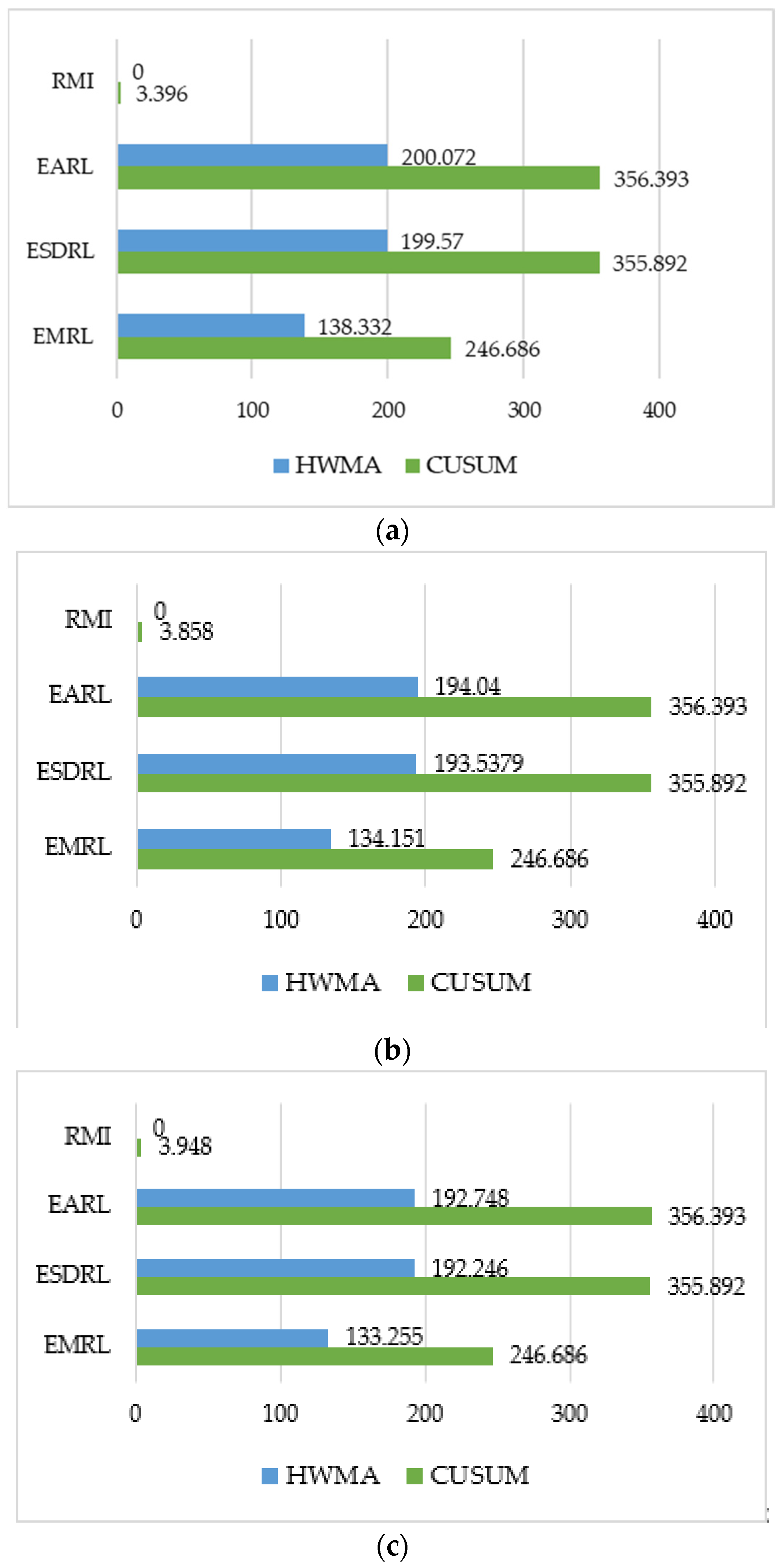
| RMI | 0 | 3.396 | 0 | 3.858 | 0 | 3. 948 | |
| EARL | 200.072 | 356.393 | 194.040 | 356.393 | 192.748 | 356.393 | |
| ESDRL | 199.570 | 355.892 | 193.5379 | 355.892 | 192.246 | 355.892 | |
| EMRL | 138.332 | 246.686 | 134.151 | 246.686 | 133.255 | 246.686 | |
| Process | Variable | Coefficient | Std. Error | t | Sig. |
|---|---|---|---|---|---|
| MAX(1,1) | MA(1) () | −0.846 | 0.103 | −8.227 | 0.00 |
| Apple Inc. stock price () | 24.429 | 0.098 | 250.237 | 0.00 | |
| MAX(2,1) | −1.222 | 0.126 | −9.695 | 0.00 | |
| −0.667 | 0.128 | −5.204 | 0.00 | ||
| Apple Inc. stock price () | 24.417 | 0.117 | 207.912 | 0.00 | |
| MAX(3,1) | −1.085 | 0.158 | −6.850 | 0.00 | |
| −0.765 | 0.211 | −3.627 | 0.00 | ||
| −0.435 | 0.165 | −2.647 | 0.01 | ||
| Apple Inc. stock price () | 24.400 | 0.131 | 186.435 | 0.00 |
| Process | RMSE | MAPE | MAE |
|---|---|---|---|
| MAX(1,1) | 58.951 | 1.120 | 46.329 |
| MAX(2,1) | 46.407 | 0.856 | 35.411 |
| MAX(3,1) | 45.571 | 0.794 | 32.829 |
| Process | Kolmogorov–Smirnov | Sig. | |
|---|---|---|---|
| MAX(3,1) | 29.42908 | 0.679 | 0.745 |
Disclaimer/Publisher’s Note: The statements, opinions and data contained in all publications are solely those of the individual author(s) and contributor(s) and not of MDPI and/or the editor(s). MDPI and/or the editor(s) disclaim responsibility for any injury to people or property resulting from any ideas, methods, instructions or products referred to in the content. |
© 2023 by the authors. Licensee MDPI, Basel, Switzerland. This article is an open access article distributed under the terms and conditions of the Creative Commons Attribution (CC BY) license (https://creativecommons.org/licenses/by/4.0/).
Share and Cite
Sunthornwat, R.; Sukparungsee, S.; Areepong, Y. Analytical Explicit Formulas of Average Run Length of Homogenously Weighted Moving Average Control Chart Based on a MAX Process. Symmetry 2023, 15, 2112. https://doi.org/10.3390/sym15122112
Sunthornwat R, Sukparungsee S, Areepong Y. Analytical Explicit Formulas of Average Run Length of Homogenously Weighted Moving Average Control Chart Based on a MAX Process. Symmetry. 2023; 15(12):2112. https://doi.org/10.3390/sym15122112
Chicago/Turabian StyleSunthornwat, Rapin, Saowanit Sukparungsee, and Yupaporn Areepong. 2023. "Analytical Explicit Formulas of Average Run Length of Homogenously Weighted Moving Average Control Chart Based on a MAX Process" Symmetry 15, no. 12: 2112. https://doi.org/10.3390/sym15122112
APA StyleSunthornwat, R., Sukparungsee, S., & Areepong, Y. (2023). Analytical Explicit Formulas of Average Run Length of Homogenously Weighted Moving Average Control Chart Based on a MAX Process. Symmetry, 15(12), 2112. https://doi.org/10.3390/sym15122112