Article

Statistical Fuzzy Reliability Analysis: An Explanation with Generalized Intuitionistic Fuzzy Lomax Distribution

Faculty of Science, Beijing University of Technology, Beijing 100124, China
*
Author to whom correspondence should be addressed.
Symmetry 2023, 15(11), 2054; https://doi.org/10.3390/sym15112054
Submission received: 18 October 2023 / Revised: 31 October 2023 / Accepted: 4 November 2023 / Published: 13 November 2023

Abstract

:
To illustrate data uncertainty, intuitionistic fuzzy sets simply use membership and non-membership degrees. However, in some cases, a more complex strategy is required to deal with imprecise data. One of these techniques is generalized intuitionistic fuzzy sets (GIFSs), which provide a comprehensive framework by adding extra factors that provide a more realistic explanation for uncertainty. GIFSs contain generalized membership, non-membership, and hesitation degrees for establishing symmetry around a reference point. In this paper, we applied a generalized intuitionistic fuzzy set approach to investigate ambiguity in the parameter of the Lomax life distribution, seeking a more symmetric assessment of the reliability measurements. Several reliability measurements and associated cut sets for a novel L-R type fuzzy sets are derived after establishing the scale parameter as a generalized intuitionistic fuzzy number. Additionally, the study includes a range of reliability measurements, such as odds, hazards, reliability functions, etc., that are designed for the Lomax distribution within the framework of generalized intuitionistic fuzzy sets. These reliability measurements are an essential tool for evaluating the reliability characteristics of various types of complex systems. For the purpose of interpretation and application, the results are visually displayed and compared across different cut set values using a numerical example.

1. Introduction

The reliability or survival analysis over time has been determined to be the most effective and efficient way for investigating lifetime data. Traditional reliability analysis, which is based on exact data, lacks the symmetry required to deal with uncertain contexts that include ambiguity, vagueness, and other forms of uncertainty. To deal with these ambiguous and uncertain data, the reliability assessment approach must be customized to the fuzzy lifetime. For this purpose, Zadeh [1] initially conceived of fuzzy sets theory to cope with ambiguity or fuzziness in data. The components of a fuzzy set are specified by their membership degree, which reflects the chance of an event occurring in order to determine the imprecision. Many extensions of fuzzy have been produced as a consequence of successful research, including rough fuzzy, type 1 fuzzy, type 2, interval valued fuzzy, and Atanassov’s intuitionistic fuzzy sets (IFSs). Fuzzy life data are more precisely modeled by intuitionistic fuzzy sets because they include the degree of hesitation margin in addition to membership and non-membership degree. Due to the fact that all real-world data involve vagueness and ambiguity, which conventional reliability theory cannot handle, fuzzy theory has shown to be a helpful tool in reliability. The field of fuzzy lifetime has experienced significant developments from several writers. The most significant of them is Atanassov’s [2] work, which transforms notions from intuitionistic fuzzy to type 1 fuzzy sets theory and offers several novel operations. To explore the sum of the support of classic intuitionistic fuzzy sets, Yager, R.R. [3] introduces q-rung orthopair fuzzy sets which were further explored as complemental fuzzy sets by Alcantud, J.C.R. [4]. Varghese and Rosario [5] then presented a variety of novel fuzzy sets, including Pendant and Octant fuzzy numbers as well as the α–cuts. The idea of fuzzy sets is extended to include intuitionistic fuzzy sets (IFSs), and Mahapatra and Roy [6] presented the notion of a triangular intuitionistic fuzzy number using this approach. The concept of IFSs has been utilized in many fields of reliability [7,8,9] and decision making [10,11,12]. Further advances are achieved by Feng [13] through the use of Minkowski score functions of intuitionistic fuzzy values and geometric ranking in a decision-making problem.
In addition, fuzzy set theory has also drawn a lot of interest in the field of system reliability analysis. For instance, Kumar, A. [14] used triangular hesitant fuzzy sets and a Markov process to verify the system’s reliability for the Weibull parameters. In a subsequent study, expanding on his previous work, Kumar, A. [15] used hesitant and dual hesitant fuzzy sets to assess fuzzy reliability. Reliability analysis of a parallel system with maximum operating and repair periods was studied by Malik and Rathee [16]. In order to develop the membership and non-membership functions, Garg, H. [17] handles the fuzzy system reliability analysis by taking into account the various intuitionistic fuzzy failure rates. The notion of a probabilistic dual hesitant fuzzy set was suggested by Hao et al. [18] in order to take additional information into consideration and explain the aleatory and epistemic ambiguity within a single framework. In addition, Refs. [19,20,21] used intuitionistic fuzzy sets to assess multi-state system and time-dependent system reliabilities. Other complex systems, including power supply distribution and data integration systems using simulation-based techniques, can be seen in [22,23,24].
The Lomax distribution, also known as the Pareto II distribution, developed by Lomax [25] has recently gained prominence in the area of life testing because of its applications in the fitting of data on business failure. This has been shown to be the best alternative to the exponential, Weibull, or gamma distributions for modeling a heavy-tailed distribution with a high decreasing failure rate [26]. The Lomax distribution has been explored in a variety of applications throughout scientific research. As an example, Pak, A. [27] estimated the parameters of Lomax distribution with fuzzy observations. Afterward, Al-Noor, N.H. [28] described the composite trapezoidal rule-based fuzzy reliability estimate for the Lomax distribution. As for the other life distribution, Baloui Jamkhaneh [29] and Kumar, P. [30] analyzed different life distributions such as Rayleigh and Weibull and gave fuzzy reliability and hazard function formulae, as well as their α–cut set. Apart from these, Cramer, E. [31] presented a vast review on life distribution to explore the different censoring schemes with the help of ordered statistics to explore the incomplete data for different reliability models.
The concept of generalized intuitionistic fuzzy sets (GIFSs) was first developed by Mondal and Samanta [32]. Baloui Jamkhaneh and Shabani [33,34] then developed a new type of generalized intuitionistic fuzzy set, which has since become a well-known method in the field of fuzzy life distribution. They used this new type of GIFS to create reliability characteristics such as reliability and hazard functions for various life distributions such as exponential, Rayleigh, and so on. In their most recent work, Roohanizadeh, Z. and Baloui Jamkhaneh [35,36] presented different reliability characteristics specially designed for a two-parameter Pareto distribution using generalized intuitionistic fuzzy sets. The available literature makes it abundantly evident that understanding fuzzy reliability for fuzzy life distribution is critical from both a theoretical and a real-world perspective.
For this purpose, we considered the Lomax distribution, which exhibits uncertainty in the scale parameter, and we fuzzified this parameter into a generalized intuitionistic fuzzy number. The main objective of this article is to introduce a novel L-R type fuzzy approach and the corresponding cut sets, which can effectively elucidate the vagueness inherent in various generalized intuitionistic fuzzy reliability measures. The goal of developing this new methodology is to improve reliability evaluations and understanding of complex systems, especially when uncertainty and imprecision are significant factors.
The rest of the paper is organized as follows: Section 2 introduces the fundamental concepts of generalized intuitionistic fuzzy set theory. In Section 3, generalized intuitionistic fuzzy parameters are used to discuss the major reliability features such as reliability, hazard, and odds functions for Lomax life distribution. Finally, a numerical example and its graphic representation to support the theoretical aspects are discussed in Section 4.

2. Definitions

2.1. Generalized Intuitionistic Fuzzy Set (GIFS)

A more sophisticated form of the intuitionistic fuzzy set [37], referred to as the generalized intuitionistic fuzzy set (GIFS), was developed by Baloui Jamkhaneh and Nadarajah. [33]. According to them, a GIFS B ¯ in non-empty set X is defined as
B ¯ = x , μ B ¯ x , γ B ¯ x : x X ,
where the mappings μ B ¯ : X [ 0 , 1 ] , γ B ¯ : X [ 0 , 1 ] are defining the extent of membership and non-membership functions of X in B ¯ with some boundary conditions 0 μ ε B ¯ x + γ ε B ¯ x 1 and ε = n ( or 1 n ) for all x X & n = 1 , 2 , 3 , , N .

2.2. Generalized Intuitionistic Fuzzy Number (GIFN)

A generalized intuitionistic fuzzy number (GIFN) B ¯ based on the generalized intuitionistic fuzzy set (GIFS) in the form of a left and right basis is defined as [34]
μ B ¯ ( x ) = f L ( x ) , x [ a 1 , b 1 ] u , x [ b 1 , c 1 ] f R ( x ) , x [ c 1 , d 1 ] 0 , o . w ,           γ B ¯ ( x ) = g L ( x ) , x [ a 1 , b 1 ] w , x [ b 1 , c 1 ] g R ( x ) , x [ c 1 , d 1 ] 0 , o . w .
with the following membership μ B ¯ x and non-membership degree γ B ¯ x functions and boundary conditions: a 1 a 1 b 1 c 1 d 1 d 1 , 0 μ ε B ¯ x + γ ε B ¯ x 1 , x X .
In a GIFN, symmetry in the left and right bases indicates that on both sides of the central value, there is an equal distribution of non-membership and membership degrees.

2.3. Alpha–Beta Cut Sets of GIFN

Consider the fixed values α , β [ 0 , 1 ] with the following conditions: 0 α μ 1 ε , 0 β μ 1 ε and 0 α ε β ε 1 . Then, on the basis of an α–cut set of fuzzy set theory, the ( α , β ) –cut for a GIFN B ¯ is as follows:
B ¯ [ α , β , ε ] = x , μ B ¯ x α , γ B ¯ x β : x X .
The α –cut set for membership degree function of a GIFN B ¯ on domain of real line R is defined as
B ¯ [ α , ε ] = x , μ B ¯ x α : x X = [ L ( α ) , U ( α ) ]
where
L ( α ) = a 1 + ( b 1 a 1 ) α ε μ ,      U ( α ) = d 1 + ( d 1 c 1 ) α ε μ .
Similarly, the β –cut set for the non-membership degree function of a GIFN is
B ¯ [ β , ε ] = x , μ B ¯ x β : x X = [ L ( β ) , U ( β ) ]
where
L ( β ) = a 1 + ( b 1 a 1 ) ( 1 α ε ) 1 γ ,      U ( β ) = d 1 + ( d 1 c 1 ) ( 1 β ε ) 1 γ .
Finally, a generalized intuitionistic fuzzy number (GIFN) based on the α –cut and β –cut sets can be written as
B ¯ [ α , β , ε ] = x , μ B ¯ x α , 1 γ B ¯ x 1 β : x X
Or
B ¯ [ α , β , ε ] = B ¯ μ [ α , ε ] , B ¯ γ [ β , ε ] .

2.4. Some Operations on GIFN

Consider two GIFNs B ¯ 1 [ α , β , ε ] and B ¯ 2 [ α , β , ε ] .
  • B ¯ 1 [ α , β , ε ] B ¯ 2 [ α , β , ε ] = B ¯ 1 μ [ α , ε ] B ¯ 2 μ [ β , ε ] , B ¯ 1 γ [ α , ε ] B ¯ 2 γ [ β , ε ] ,
  • k B ¯ [ α , β , ε ] b 1 = k B ¯ μ [ α , ε ] b 1 , k B ¯ γ [ β , ε ] b 1 ,
  • B ¯ 1 [ α , β , ε ] = B ¯ 2 [ α , β , ε ] i f f B ¯ 1 μ [ α , ε ] = B ¯ 2 μ [ α , ε ] and B ¯ 1 γ [ β , ε ] = B ¯ 2 γ [ β , ε ] ,
  • B ¯ 1 [ α , β , ε ] = B ¯ 2 [ α , β , ε ] i f f B ¯ 1 μ [ α , ε ] = B ¯ 2 μ [ α , ε ] and B ¯ 1 γ [ β , ε ] = B ¯ 2 γ [ β , ε ] .

3. Model Description

3.1. Generalized Intuitionistic Fuzzy (GIF) Reliability Characteristics

If the lifetime of a unit is defined as random variable X with density function f ( x , θ ¯ ) , the vectors of the parameters θ ¯ are fuzzified as a generalized intuitionistic fuzzy number (GIFN). Then, the α –cut of membership and β –cut set of non-membership functions for any GIF reliability measure g ¯ ( t ) are denoted by
g i ( t ) [ j , ε ] = g ( t ) | θ θ i [ j , ε ] , ( i , j ) = ( 1 , μ ) , ( 2 , γ ) = g i L ( t ) [ j ] , g i U ( t ) [ j ] ,
where
g i L ( t ) [ j ] = inf θ θ j [ α , ε ] g ( t ) , g i L ( t ) [ j ] = sup θ θ j [ α , ε ] g ( t ) .
with constraint 0 α μ 1 ε , γ 1 ε β 1 , 0 α ε + β ε 1 and t > 0 .
The function g ( t ) can be considered as any reliability characteristic such as reliability, hazard, or odds functions. The rationale behind constructing GIF reliability analysis is, for every special value of α and β , the shapes of g i ( t ) [ α , j ] behave like bands which are nothing but the uncertainty in the parameter. Also, the GIF functions can be constructed for every special time t c .
Ref. [35] shows that g [ α , β , ε ] = { g μ ( t ) [ α , ε ] , g γ ( t ) [ β , ε ] } and he defined the ( α , β ) –cut set of GIF characteristics as
g [ α , β , ε ] = { w | w g μ ( t ) [ α , ε ] g γ ( t ) [ β , ε ] } .
Remark 1:
There are some important properties processed by reliability characteristic  g ( t ) , as follows.
  • If  μ 1 μ 2  and  γ 1 γ 2 , then  g μ 1 ( t ) [ α , ε ] g μ 2 ( t ) [ α , ε ] a n d g γ 2 ( t ) [ β , ε ] g γ 1 ( t ) [ β , ε ] ,
  • If  ε 1 ε 2 , then  g μ ( t ) [ α , ε 1 ] g μ ( t ) [ α , ε 1 ] a n d g γ ( t ) [ β , ε 2 ] g γ ( t ) [ β , ε 2 ] .

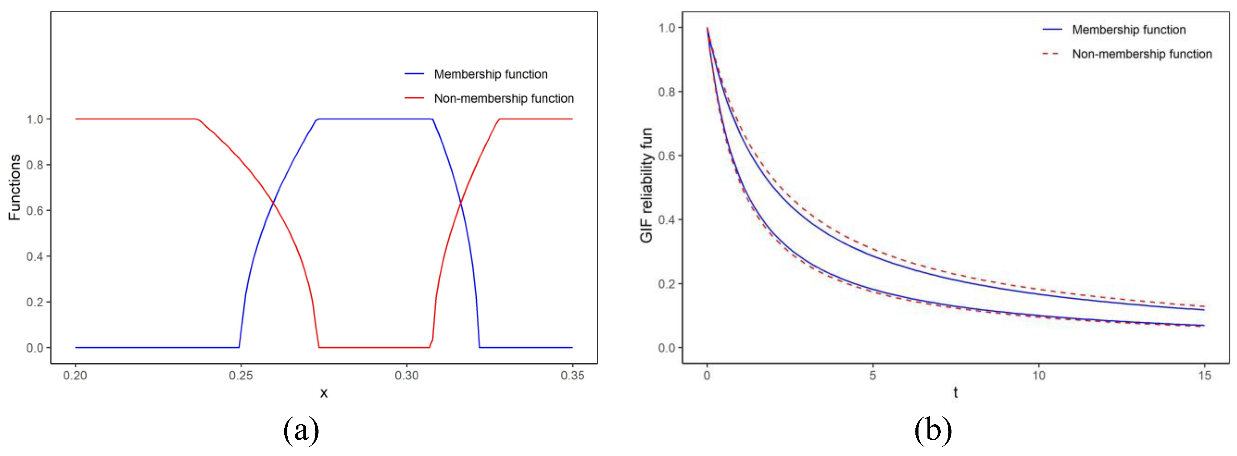
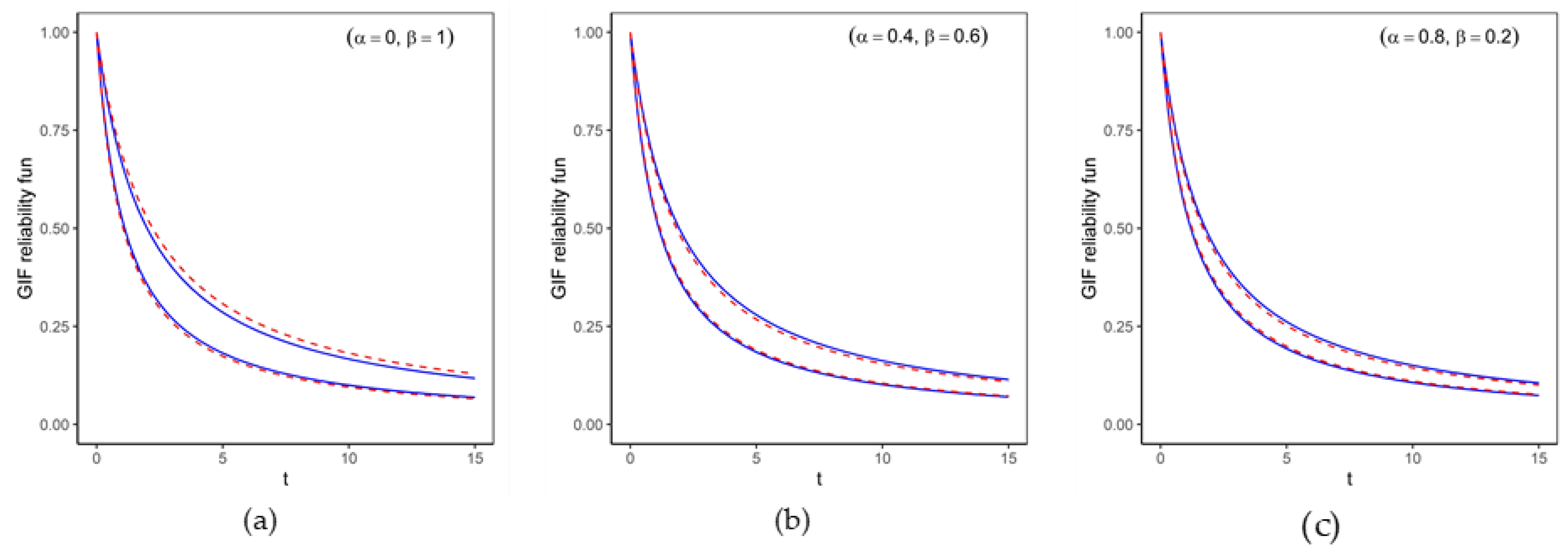
3.2. GIF Reliability Function

In this section, the lifetime generalized intuitionistic fuzzy number (GIFN) parameter is used to develop a notion of the generalized intuitionistic fuzzy reliability function, represented as R ¯ ( t ) .
The α –cut of membership and β –cut set of non-membership functions are
R i ( t ) [ j , ε ] = R ( t ) | θ θ i [ j , ε ] , ( i , j ) = ( 1 , μ ) , ( 2 , γ ) = R i L ( t ) [ j ] , R i U ( t ) [ j ]
where
R i L ( t ) [ j ] = inf θ θ i [ j , ε ] R ( t ) , R i L ( t ) [ j ] = sup θ θ i [ j , ε ] R ( t ) ,      0 α ε + β ε 1 .
The ( α , β ) –cut set of GIF reliability function is as follows:
R ( t ) [ α , β , ε ] = w | w R μ ( t ) [ α , ε ] R γ ( t ) [ β , ε ] .
More specifically, the Lomax distribution has been considered, and the relevant reliability characteristics are provided. Suppose a random variable X from the Lomax life distribution with CDF
F ( x ) = 1 ( 1 + θ x ) η ,         x , θ , η > 0 ,
and PDF
f ( x , λ ) = η θ ( 1 + θ x ) ( η + 1 ) ,        x , θ , η > 0 ,
which has fixed shape parameter η and uncertainty in scale parameter θ that is well explained by fuzzifying the uncertain parameter into a GIFN. Hence, the GIF scale parameter for fuzzification is taken as
θ ¯ = ( a 1 , a 1 , b 1 , c 1 , d 1 , d 1 , μ , γ , ε )
now, the cut set of the generalized intuitionistic fuzzy reliability function can be obtained as reliability bands
R i ( t ) [ j , ε ] = [ ( 1 + θ t ) η | θ θ i [ j , ε ] , ( i , j ) = ( 1 , α ) , ( 2 , β ) ] .
Since the function ( 1 + θ t ) η is monotonically decreasing with respect to θ , the cut sets for reliability bands are given as
R μ ( t ) [ α , ε ] = 1 + U ( α ) t η , 1 + L ( α ) t η
R γ ( t ) [ β , ε ] = 1 + U ( β ) t η , 1 + L ( β ) t η .
Or
R μ ( t ) [ α , ε ] = 1 + d 1 ( d 1 c 1 ) α ε μ t η , 1 + a 1 + ( b 1 a 1 ) α ε μ t η
R γ ( t ) [ β , ε ] = 1 + d 1 ( d 1 c 1 ) ( 1 β ε ) 1 γ t η , 1 + a 1 + ( b 1 a 1 ) ( 1 β ε ) 1 γ t η .
For every specific value of α and β , reliability bands must satisfy the following properties:
  • R i ( 0 ) [ j , ε ] = [ 1 , 1 ] ,
  • R i ( ) [ j , ε ] = [ 0 , 0 ] ,
  • R i ( t 1 ) R i ( t 2 ) i f f t 1 t 2 .
Since R i ( t ) [ j , ε ] varies with time t, then for every special set of α , β and time t = t c , its membership μ R ( t c ) ( x ) and non-membership γ R ( t c ) ( x ) functions are given as
μ R ( t c ) ( x ) = d 1 x 1 η 1 t c μ d 1 c 1 1 ε , x ( 1 + d 1 t c ) η , ( 1 + c 1 t c ) η μ 1 ε , x ( 1 + c 1 t c ) η , ( 1 + b 1 t c ) η x 1 η 1 t c a 1 μ b 1 a 1 1 ε , x ( 1 + b 1 t c ) η , ( 1 + a 1 t c ) η 0 , o . w ,
γ R ( t c ) ( x ) = d 1 c 1 ( 1 γ ) x 1 η 1 t c d 1 d 1 c 1 1 ε , x ( 1 + d 1 t c ) η , ( 1 + c 1 t c ) η γ 1 ε , x ( 1 + c 1 t c ) η , ( 1 + b 1 t c ) η b 1 a 1 + ( 1 γ ) a 1 x 1 η 1 t c b 1 a 1 1 ε , x ( 1 + b 1 t c ) η , ( 1 + a 1 t c ) η 1 , o . w
with constraint μ + γ 1 , μ R ( t c ) ( x ) and 1 γ R ( t c ) ( x ) are fuzzy numbers.

3.3. GIF Conditional Reliability Function

The likelihood that an object will survive at time t, assuming that it has survived up to that point (T), is known as conditional reliability. Here, we apply the generalized intuitionistic fuzzy idea to expand the conditional reliability measure to the ambiguous case. The α –cut and β –cut sets for GIF conditional reliability functions are given by the following expression:
R i ( t | T ) [ j , ε ] = R ( t | T ) | θ θ i [ j , ε ] , ( i , j ) = ( 1 , μ ) , ( 2 , γ ) = R i L ( t | T ) [ j ] , R i U ( t | T ) [ j ]
where
R i L ( t | T ) [ j ] = inf θ θ i [ j , ε ] R ( t | T ) ,     R i L ( t | T ) [ j ] = sup θ θ i [ j , ε ] R ( t | T )
and the ( α , β ) –cut set of the GIF conditional reliability function is derived as
R ( t | T ) [ α , β , ε ] = w | w R μ ( t | T ) [ α , ε ] R γ ( t | T ) [ β , ε ] .
The GIF conditional reliability function for the Lomax distribution can be modified as
R i ( t | T ) [ j , ε ] = 1 + θ T 1 + θ t η | θ θ i [ j , ε ] , ( i , j ) = ( 1 , μ ) , ( 2 , γ ) .
Function 1 + θ T 1 + θ T η is monotonically decreasing with respect to θ which leads to the following expression for GIF conditional reliability bands:
R μ ( t | T ) [ j , ε ] = 1 + d 1 ( d 1 c 1 ) α ε μ T 1 + d 1 ( d 1 c 1 ) α ε μ t η , 1 + a 1 + ( b 1 a 1 ) α ε μ T 1 + a 1 + ( b 1 a 1 ) α ε μ t η ,
R γ ( t | T ) [ j , ε ] = 1 + d 1 ( d 1 c 1 ) ( 1 β ε ) 1 γ ε T 1 + d 1 ( d 1 c 1 ) ( 1 β ε ) 1 γ t η , 1 + a 1 + ( b 1 a 1 ) ( 1 β ε ) 1 γ T 1 + a 1 + ( b 1 a 1 ) ( 1 β ε ) 1 γ t η .

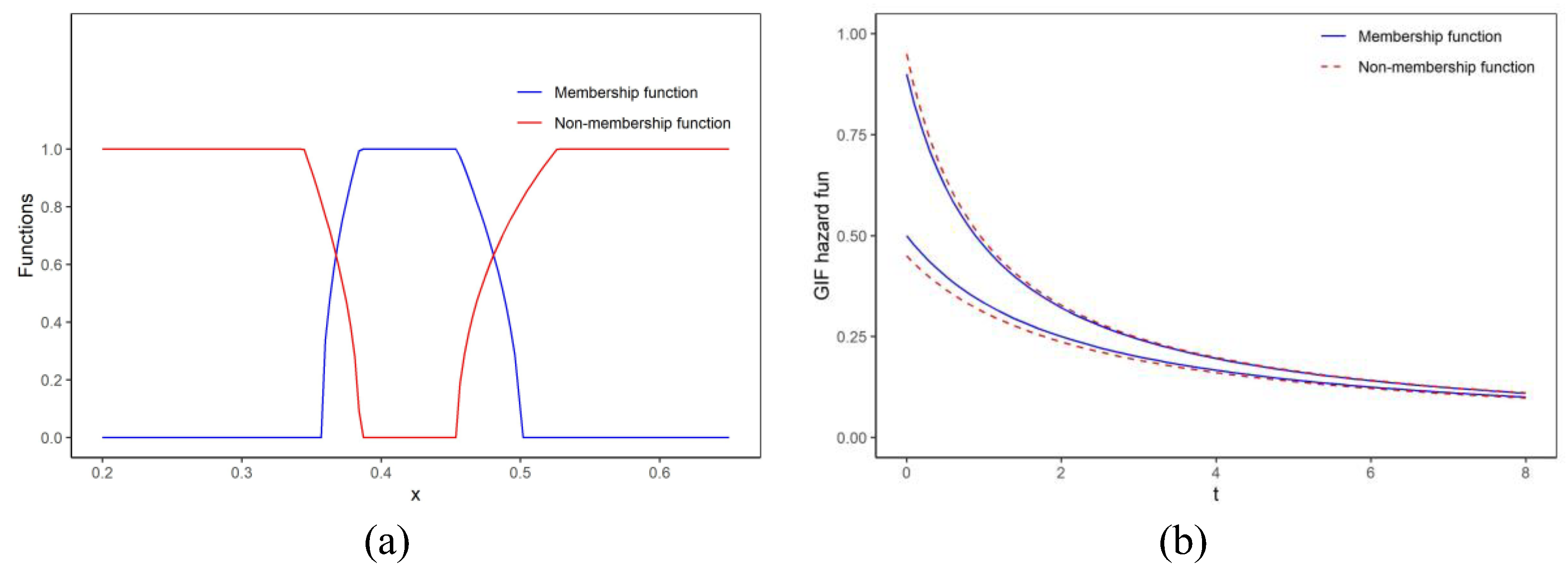
3.4. GIF Hazard Function

The hazard function, often known as the instant failure rate, is another important part of the lifespan distribution. This function indicates the rate of failure at which a component is projected to fail after a specific time of service. The α and β cut sets of GIF hazard functions are
h i ( t ) [ j , ε ] = h ( t ) | θ θ i [ j , ε ] , ( i , j ) = ( 1 , μ ) , ( 2 , γ ) = h i L ( t ) [ j ] , h i U ( t ) [ j ]
where
h i L ( t ) [ j ] = inf θ θ i [ j , ε ] h ( t ) ,        h i L ( t ) [ j ] = sup θ θ i [ j , ε ] h ( t )
And the ( α , β ) –cut set for the GIF hazard function is derived as
h ( t ) [ α , β , ε ] = w | w h μ ( t ) [ α , ε ] h γ ( t ) [ β , ε ] .
For the Lomax distribution, the above GIF hazard function can be modified as
h i ( t ) [ j , ε ] = θ η 1 + θ t | θ θ i [ j , ε ] , ( i , j ) = ( 1 , μ ) , ( 2 , γ ) .
Since θ η 1 + θ t is monotonically increasing with parameter θ , the hazard bands are given as
h μ ( t ) [ j , ε ] = a 1 + ( b 1 a 1 ) α ε μ η 1 + a 1 + ( b 1 a 1 ) α ε μ t , d 1 ( d 1 c 1 ) α ε μ η 1 + d 1 ( d 1 c 1 ) α ε μ t ,
h γ ( t ) [ j , ε ] = a 1 + ( b 1 a 1 ) ( 1 β ε ) 1 γ η 1 + a 1 + ( b 1 a 1 ) ( 1 β ε ) 1 γ t , d 1 ( d 1 c 1 ) ( 1 β ε ) 1 γ η 1 + d 1 ( d 1 c 1 ) ( 1 β ε ) 1 γ t .
Corollary 1:
Let us consider the two lifetime random variables  T 1  and  T 2  having generalized intuitionistic fuzzy density function  f 1 x , θ ¯ , η  and  f 2 x , θ ¯ , η , respectively. For every  t > 0 , if the conditions  h ¯ 1 ( t ) h ¯ 2 ( t ) a n d R ¯ 1 ( t ) = R ¯ 2 ( t )  hold, it can be proven that  R ¯ 1 ( t | T ) R ¯ 2 ( t | T ) .
Theorem 1:
The function  R ¯ ( x | t )  must be increasing for  f x , θ ¯ , η  to belong to a class of decreasing failure rate distribution, which is a necessary and sufficient condition.
Proof: 
As discussed,
R ¯ ( x | t 1 ) R ¯ ( x | t 2 ) , t 1 < t 2   and   R ¯ ( x | t 1 ) [ α , β , ε ] R ¯ ( x | t 2 ) [ α , β , ε ] ,
So,
R 1 μ ( x | t 1 ) [ α , ε ] , R 1 γ ( x | t 2 ) [ β , ε ] R 2 μ ( x | t 2 ) [ α , ε ] , R 2 γ ( x | t 2 ) [ β , ε ] ,
Or
R 1 μ ( x | t 1 ) [ α , ε ] R 2 μ ( x | t 2 ) [ α , ε ] and R 1 γ ( x | t 1 ) [ β , ε ] R 2 γ ( x | t 2 ) [ β , ε ] .
Taking lower band = upper band = b , then, for every b ,
R γ b ( x | t 1 ) [ α , ε ] R γ b ( x | t 2 ) [ α , ε ] and R γ b ( x | t 1 ) [ β , ε ] R γ b ( x | t 2 ) [ β , ε ] .
which indicates that R μ b and R γ b are increasing functions.
Now, using the definition of the GIF conditional survival function for ( i , j ) = ( 1 , μ ) , ( 2 , γ ) ,
R i b ( x | t ) [ j , ε ] = R i b ( x + t ) [ j , ε ] R i b ( t ) [ j , ε ] ,
d R i b ( x | t ) [ j , ε ] d t = f i b ( x + t ) [ j , ε ] R i b ( t ) [ j , ε ] + f i b ( t ) [ j , ε ] R i b ( x + t ) [ j , ε ] R i b ( t ) [ j , ε ] 2 .
Since R i b has increasing shape, so the function d R i b ( x | t ) [ j , ε ] d t 0 and
f i b ( x + t ) [ j , ε ] R i b ( t ) [ j , ε ] f i b ( t ) [ j , ε ] R i b ( x + t ) [ j , ε ] ,
hence,
h i b ( t ) [ j , ε ] h i b ( x + t ) [ j , ε ] ,
Or
h μ b ( t ) [ j , ε ] h μ b ( x + t ) [ j , ε ] and h γ b ( t ) [ j , ε ] h γ b ( x + t ) [ j , ε ] ,
Finally, it can be concluded that h ¯ ( t ) h ¯ ( x + t ) . □

3.5. GIF Odds Function

The odds function is a reliability method for modeling a data set with a non-monotone hazard rate, defined as the ratio of the CDF to the reliability function. As the hazard function of the Lomax distribution is often a non-monotone function, the cut set of the GIF odds function is
O i ( t ) [ j , ε ] = O ( t ) | θ θ i [ j , ε ] , ( i , j ) = ( 1 , μ ) , ( 2 , γ ) = O i L ( t ) [ j ] , O i U ( t ) [ j ]
where
O i L ( t ) [ j ] = inf θ θ i [ j , ε ] O ( t ) ,       O i L ( t ) [ j ] = sup θ θ i [ j , ε ] O ( t )
Therefore,
O i ( t ) [ j , ε ] = F i ( t ) [ j , ε ] S i ( t ) [ j , ε ] | θ θ i [ j , ε ] , ( i , j ) = ( 1 , μ ) , ( 2 , γ ) = ( 1 + θ t ) η 1 | θ θ i [ j , ε ] , ( i , j ) = ( 1 , μ ) , ( 2 , γ ) ,
which can be modified for the Lomax distribution as
O μ ( t ) [ j , ε ] = 1 + a 1 + ( b 1 a 1 ) α ε μ t η 1 , 1 + ( d 1 ( d 1 c 1 ) α ε μ ) t η 1 ,
O γ ( t ) [ j , ε ] = 1 + a 1 + ( b 1 a 1 ) ( 1 β ε ) 1 γ t η 1 , 1 + d 1 ( d 1 c 1 ) ( 1 β ε ) 1 γ t η 1 .

4. Numerical Illustration

The Lomax distribution could be considered to model long-duration failure devices, for instance, network switches that can fail due to various reasons such as power supply, extreme temperature, aging, or manufacturing issues. Let us consider the lifetime of network switches that are modelled by a Lomax distribution with generalized intuitionistic fuzzy scale parameter θ ¯ = ( 0 . 45 , 0 . 5 , 0 . 6 , 0 . 8 , 0 . 9 , 0 . 95 , 1 , 0 , 2 ) and shape parameter η = 1 .
Then, the α and β cut sets of membership and non-membership for generalized intuitionistic fuzzy reliability functions for t = 2 can be derived as
R μ ( t ) [ α , 2 ] = 1 1 + 0.9 0.1 α 2 t , 1 1 + 0.5 + 0.1 α 2 t ,
R γ ( t ) [ β , 2 ] = 1 1 + 0.8 + 0.15 β 2 t , 1 1 + 0.6 0.15 β 2 t .
The above reliability functions behave as lower and upper bands, and the value of the bandwidth depends on the value of α , β .
The GIF reliability bands with their corresponding lower and upper reliability bands for different sets of α , β values are shown in Table 1, where R μ ( t ) [ α , 2 ] is the α cut of membership functions, R γ ( t ) [ β , 2 ] is the β cut as of non-membership functions, and R ( t ) [ α , β , 2 ] indicates their intersection as a α , β –cut sets.
The membership and non-membership functions for GIF reliability bands at t = 2 and α = 0 , β = 1 are shown in Figure 1a. And Figure 1b indicates the GIF reliabilities bands are decreasing with respect to time t for α = 0 , β = 1 .
For a more precise view, Figure 2a–c display a few more sets of α , β values, which clearly indicate that increasing α and decreasing β simultaneously reduce the bandwidth (fuzziness) of both membership and non-membership functions.
As mentioned earlier, the reliability function must show its GIF nature for every special set of α , β and time t. Hence, the membership and non-membership functions for GIF reliability bands at t = 2 can be found and are shown in Figure 1a.
μ R ( 2 ) ( x ) = 0.8 x 1 0.2 0.5 , x 0.3571 , 0.3846 1 , x 0.3846 , 0.4545 x 1 2 0.2 0.5 , x 0.4545 , 0.5000 0 , o . w , γ R ( 2 ) ( x ) = 3.05 x 1 0.3 0.5 , x 0.3448 , 0.4545 0 , x 0.4545 , 0.3846 2.05 x 1 0.3 0.5 , x 0.3846 , 0.5263 1 , o . w .
Similarly, the cut sets for generalized intuitionistic fuzzy conditional reliability bands are given by the following formulas and calculated in Table 2 for various sets of values.
R μ ( t | T ) [ α , 2 ] = 1 + 0.9 0.1 α 2 T 1 + 0.9 0.1 α 2 t 1 , 1 + 0.5 + 0.1 α 2 T 1 + 0.5 + 0.1 α 2 t 1 ,
R γ ( t | T ) [ β , 2 ] = 1 + 0.8 + 0.15 β 2 T 1 + 0.8 + 0.15 β 2 t 1 , 1 + 0.6 0.15 β 2 T 1 + 0.6 0.15 β 2 t 1 .
Furthermore, the membership and non-membership functions for GIF conditional reliability bands for α = 0 , β = 1 and t = 2 can be seen in Figure 3a and there is also a decreasing trend of GIF conditional reliability bands with time t in Figure 3b.
The cut sets of generalized intuitionistic hazard bands are presented in Table 3 using the formulae described below.
h μ ( t ) [ j , ε ] = 0.5 + 0.1 α 2 1 + 0.5 + 0.1 α 2 t , 0.9 0.1 α 2 1 + 0.9 0.1 α 2 t ,
h γ ( t ) [ j , ε ] = 0.6 0.15 β 2 1 + 0.6 0.15 β 2 t , 0.8 + 0.15 β 2 1 + 0.8 + 0.15 β 2 t .
In the same way, Figure 4a depicts the GIF curves for membership and non-membership values of hazard bands. And Figure 4b indicates that the decreasing GIF hazard rate with time t and least vagueness can be seen with the highest and lowest values of α and β , respectively.
Furthermore, the generalized intuitionistic fuzzy hazard functions, along with their respective membership and non-membership degree functions at t = 2 and α = 0 and β = 1 , can be viewed as
μ h ( t c ) ( x ) = x 1 1.9 0.2 0.5 , x 0.3333 , 0.3750 1 , x 0.3750 , 0.4444 3.8 x 1 0.2 0.5 , x 0.4444 , 0.4736 0 o . w ,
γ h ( t c ) ( x ) = 2.2 x 1 0.3 0.5 , x 0.3103 , 0.3750 0 , x 0.3750 , 0.4444 x 1 2.6 0.3 0.5 , x 0.4444 , 0.4871 1 , o . w .
The α , β cut sets of generalized intuitionistic fuzzy odds bands with their respective lower and upper bands are presented in Table 4 as:
O μ ( t ) [ j , ε ] = 0.5 + 0.1 α 2 t , 0.9 0.1 α 2 t ,
O γ ( t ) [ j , ε ] = 0.6 0.15 β 2 t , 0.8 + 0.15 β 2 t .
Analogously, the GIF curves for the odds band are displayed in Figure 5a, and the rapid growth of the odds band with time reference can be observed in Figure 5b.
The α , β cut sets of generalized intuitionistic.
The membership and non-membership functions for GIF odds functions at fixed t = 2 are as follows:
O h ( t c ) ( x ) = x 1 0.2 0.5 , x 1 , 1.2 1 , x 1.2 , 1.6 1.8 x 0.2 0.5 , x 1.6 , 1.8 0 , o . w ,       O h ( t c ) ( x ) = 1.2 x 0.3 0.5 , x 0.9 , 1.2 0 , x 1.2 , 1.6 x 1.6 0.3 0.5 , x 1.6 , 1.9 1 , o . w

5. Results and Discussion

This study presents a novel method for applying generalized intuitionistic fuzzy approaches to the Lomax lifespan distribution. The primary goal of this work is to evaluate the degree of uncertainty inherent in various reliability factors. This is achieved by quantifying the fuzziness in scale parameter θ ¯ : ( a 1 = 0 . 45 , a 1 = 0 . 5 , b 1 = 0 . 6 , c 1 = 0 . 8 , d 1 = 0 . 9 , d 1 = 0 . 95 ) of the Lomax life distribution. In terms of the fuzzy approach, we focused on a specific instance of the generalized intuitionistic fuzzy framework that included specified values for μ = 1 , γ = 0 . In this case, we used ε = 2 and the cut set method to compute the bands for different reliability measurements.
The ( α , β ) cut bands of the GIF reliability function for different sets of ( α , β ) are calculated in Table 1. Also, these reliability bands for three different sets of ( α , β ) are graphically depicted in Figure 2. On the basis of Table 1 and Figure 2, the most reduced bandwidths of membership and non-membership bands are seen at the greatest α and lowest values of β , indicating that increasing α and reducing β lead to a decline in the vagueness of reliability bands. As reliability characteristics also vary with time, Figure 1b shows that the reliability bands are decreasing with respect to time t. Another reliability characteristic is that conditional reliability bands for T = 1, as shown in Figure 3b, indicate that an increase in time t results in an increase in bandwidth or fuzziness. Meanwhile, Table 2 with respect to ( α , β ) cut sets indicates that an increase in α and decrease in β lead to reduced fuzziness in the conditional reliability function.
Apart from the bands, we also present the generalized intuitionistic fuzzy (GIF) membership and non-membership functions (MFs and NMFs) for every reliability measurement in Figure 1, Figure 2, Figure 3, Figure 4 and Figure 5.
For example, for the GIF hazard functions displayed in Figure 4a, a blue line indicates membership functions and a red line non-membership function. Also, the GIF hazard bands for the set of ( α , β ) are presented in Table 3 and graphically displayed for α = 0 ,   β = 1 in Figure 4b, which shows that increasing t leads to more accurate bandwidth for GIF hazard functions. Similarly, the odds function, the last characteristic, is computed as the ratio of two reliability features, as shown in the accompanying Figure 5b. It depicts a clear and straightforward relationship, suggesting that uncertainty rises proportionally with the passage of time t. Table 4 illustrates the fact that the ambiguity in the odds function can only be reduced by simultaneously modifying and adjusting the values of ( α , β ) .
Finally, Table 1, Table 2, Table 3 and Table 4 show that increasing α and decreasing β lead to narrower and more accurate bands for various reliability measures such as the reliability function, conditional reliability function, hazard function, and odds function. Notably, all the reliability metrics demonstrate a falling trend concerning t, except for the odds function. Exploring the effects of these changes on system reliability as a future research direction could yield significant insights.

6. Conclusions

In this paper, the notion of generalized intuitionistic fuzzy sets is used to assess the reliability of the Lomax lifetime distribution. In order to derive various generalized intuitionistic fuzzy reliability measures, the scale parameter of the Lomax distribution is regarded as a generalized intuitionistic fuzzy number. The reliability measurements are viewed as a band and their fuzziness is equal to the bandwidth for each unique pair of cut set values. The findings show that the most exact bandwidths are obtained when the cut set of membership functions is high and the cut set of non-membership functions is low. Notably, this technique outperforms other fuzzy sets in terms of revealing higher ambiguity. Future research on the subject of system reliability, particularly in the context of series and parallel arrangements, will provide an opportunity to improve on the current paradigm. Also, one can explore additional characteristics such as cumulative hazard, reversed hazard, mean time to failure, and mean past lifetime functions within the framework of the generalized intuitionistic fuzzy lifetime distribution. This investigation may provide useful insights and a more complete understanding of system behaviour and reliability in complicated network systems.
It is necessary to recognize some restrictions related to the application of the generalized intuitionistic fuzzy technique in reliability analysis. When working with generalized intuitionistic fuzzy numbers, a significant limitation is the greater degree of difficulty in modeling and computing, which can possibly cause issues in real-world applications. These difficulties emphasize the importance of additional study to overcome these challenges in real-world reliability analysis.

Author Contributions

Conceptualization, A.K. and W.C.; methodology, A.K.; software, A.K. and Y.D.; validation, W.C. and X.Z.; formal analysis, Y.D.; investigation, W.C.; data curation, A.K.; writing—original draft preparation, A.K. and W.C.; writing—review and editing, W.C. and X.Z.; visualization, Y.D.; supervision, W.C.; project administration, W.C. and X.Z.; funding acquisition, W.C. All authors have read and agreed to the published version of the manuscript.

Funding

This work was supported by the Beijing Natural Science Foundation (grant no. Z190021).

Data Availability Statement

Data sets are available in this article.

Conflicts of Interest

The authors declare no conflict of interest.

References

  1. Zadeh, L.A. Fuzzy sets. Inf. Control 1965, 8, 338–353. [Google Scholar] [CrossRef]
  2. Atanassov, K.T. Type-1 fuzzy sets and intuitionistic fuzzy sets. Algorithms 2017, 10, 106. [Google Scholar] [CrossRef]
  3. Yager, R.R. Generalized orthopair fuzzy sets. IEEE Trans. Fuzzy Syst. 2016, 25, 1222–1230. [Google Scholar] [CrossRef]
  4. Alcantud, J.C.R. Complemental Fuzzy Sets: A Semantic Justification of $ q $-Rung Orthopair Fuzzy Sets. IEEE Trans. Fuzzy Syst. 2023, 1–9. [Google Scholar] [CrossRef]
  5. Varghese, P.J.; Rosario, G.M. A study on reliability using pendant, hexant, octant fuzzy numbers. J. Reliab. Stat. Stud. 2021, 491–526. [Google Scholar] [CrossRef]
  6. Mahapatra, G.; Roy, T. Reliability evaluation using triangular intuitionistic fuzzy numbers arithmetic operations. World Acad. Sci. Eng. Technol. 2009, 50, 574–581. [Google Scholar]
  7. Kumar, M.; Singh, S.; Kumar, D. System reliability analysis based on Pythagorean fuzzy set. Int. J. Math. Oper. Res. 2023, 24, 253–285. [Google Scholar] [CrossRef]
  8. Panchal, D. Reliability analysis of turbine unit using Intuitionistic Fuzzy Lambda-Tau approach. Rep. Mech. Eng. 2023, 4, 47–61. [Google Scholar] [CrossRef]
  9. Song, Y.; Wang, X.; Zhu, J.; Lei, L. Sensor dynamic reliability evaluation based on evidence theory and intuitionistic fuzzy sets. Appl. Intell. 2018, 48, 3950–3962. [Google Scholar] [CrossRef]
  10. Liao, H.; Xu, Z. Priorities of intuitionistic fuzzy preference relation based on multiplicative consistency. IEEE Trans. Fuzzy Syst. 2014, 22, 1669–1681. [Google Scholar] [CrossRef]
  11. Liu, F.; Tan, X.; Yang, H.; Zhao, H. Decision making based on intuitionistic fuzzy preference relations with additive approximate consistency. J. Intell. Fuzzy Syst. 2020, 39, 4041–4058. [Google Scholar] [CrossRef]
  12. Yang, W.; Jhang, S.T.; Fu, Z.W.; Xu, Z.S.; Ma, Z.M. A novel method to derive the intuitionistic fuzzy priority vectors from intuitionistic fuzzy preference relations. Soft Comput. 2021, 25, 147–159. [Google Scholar] [CrossRef]
  13. Feng, F.; Zheng, Y.; Alcantud, J.C.R.; Wang, Q. Minkowski weighted score functions of intuitionistic fuzzy values. Mathematics 2020, 8, 1143. [Google Scholar] [CrossRef]
  14. Kumar, A.; Singh, S.; Ram, M. Systems reliability assessment using hesitant fuzzy set. Int. J. Oper. Res. 2020, 38, 1–18. [Google Scholar] [CrossRef]
  15. Kumar, A.; Bisht, S.; Goyal, N.; Ram, M. Fuzzy reliability based on hesitant and dual hesitant fuzzy set evaluation. Int. J. Math. Eng. Manag. Sci. 2021, 6, 166. [Google Scholar] [CrossRef]
  16. Malik, S.; Rathee, R. Reliability modelling of a parallel system with maximum operation and repair times. Int. J. Oper. Res. 2016, 25, 131–142. [Google Scholar] [CrossRef]
  17. Garg, H. A novel approach for analyzing the reliability of series-parallel system using credibility theory and different types of intuitionistic fuzzy numbers. J. Braz. Soc. Mech. Sci. Eng. 2016, 38, 1021–1035. [Google Scholar] [CrossRef]
  18. Hao, Z.; Xu, Z.; Zhao, H.; Su, Z. Probabilistic dual hesitant fuzzy set and its application in risk evaluation. Knowl.-Based Syst. 2017, 127, 16–28. [Google Scholar] [CrossRef]
  19. Akbari, M.G.; Hesamian, G. Time-dependent intuitionistic fuzzy system reliability analysis. Soft Comput. 2020, 24, 14441–14448. [Google Scholar] [CrossRef]
  20. Chachra, A.; Kumar, A.; Ram, M.; Triantafyllou, I.S. Statistical Fuzzy Reliability Assessment of a Blended System. Axioms 2023, 12, 419. [Google Scholar] [CrossRef]
  21. Bhandari, A.S.; Kumar, A.; Ram, M. Fuzzy reliability evaluation of complex systems using intuitionistic fuzzy sets, in Advancements in Fuzzy Reliability Theory. IGI Global 2021, 166–180. [Google Scholar]
  22. Faulin, J.; Juan, A.A.; Martorell, S.; Ramírez-Márquez, J.-E. (Eds.) Simulation Methods for Reliability and Availability of Complex Systems; Springer: Berlin/Heidelberg, Germany, 2010; Volume 315. [Google Scholar] [CrossRef]
  23. Glushkov, A. Methods of a Chaos Theory; Astroprint: Odessa, Ukraine, 2012. [Google Scholar]
  24. Shalizi, C.R. Methods and techniques of complex systems science: An overview. Complex Syst. Sci. Biomed. 2006, 33–114. [Google Scholar]
  25. Lomax, K.S. Business failures: Another example of the analysis of failure data. J. Am. Stat. Assoc. 1954, 49, 847–852. [Google Scholar] [CrossRef]
  26. Bryson, M.C. Heavy-tailed distributions: Properties and tests. Technometrics 1974, 16, 61–68. [Google Scholar] [CrossRef]
  27. Pak, A.; Mahmoudi, M.R. Estimating the parameters of Lomax distribution from imprecise information. J. Stat. Theory Appl. 2018, 17, 122–135. [Google Scholar] [CrossRef]
  28. Al-Noor, N.H. On the Fuzzy Reliability Estimation for Lomax Distribution; AIP Publishing LLC: Melville, NY, USA, 2019. [Google Scholar] [CrossRef]
  29. Baloui, J.E. Analyzing system reliability using fuzzy Weibull lifetime distribution. 2014. Int. J. Appl. Oper. Res. 2014, 4, 93–102. [Google Scholar]
  30. Kumar, P.; Singh, S. Fuzzy system reliability using intuitionistic fuzzy Weibull lifetime distribution. Int. J. Reliab. Appl. 2015, 16, 15–26. [Google Scholar]
  31. Cramer, E. Ordered and censored lifetime data in reliability: An illustrative review. Wiley Interdiscip. Rev. Comput. Stat. 2023, 15, e1571. [Google Scholar] [CrossRef]
  32. Mondal, T.K.; Samanta, S. Generalized intuitionistic fuzzy sets. J. Fuzzy Math. 2002, 10, 839–862. [Google Scholar]
  33. Jamkhaneh, E.B.; Nadarajah, S. A new generalized intuitionistic fuzzy set. Hacet. J. Math. Stat. 2015, 44, 1537–1551. [Google Scholar] [CrossRef]
  34. Shabani, A.; Jamkhaneh, E.B. A new generalized intuitionistic fuzzy number. J. Fuzzy Set Valued Anal. 2014, 24, 1–10. [Google Scholar] [CrossRef]
  35. Roohanizadeh, Z.; Jamkhaneh, E.B.; Deiri, E. The reliability analysis based on the generalized intuitionistic fuzzy two-parameter Pareto distribution. Soft Comput. 2023, 27, 3095–3113. [Google Scholar] [CrossRef] [PubMed]
  36. Roohanizadeh, Z.; Jamkhaneh, E.B.; Deiri, E. A novel approach for analyzing system reliability using generalized intuitionistic fuzzy Pareto lifetime distribution. J. Math. Ext. 2021, 16. [Google Scholar]
  37. Atanassov, K.T.; Stoeva, S. Intuitionistic fuzzy sets. Fuzzy Sets Syst. 1986, 20, 87–96. [Google Scholar] [CrossRef]
Figure 1. (a) The MF and NMF of GIF reliability function; (b) The GIF reliability bands for α = 0 , β = 1 .
Symmetry 15 02054 g001
Figure 2. (a) Reliability bands for α = 0 , β = 1 ; (b) Reliability bands for α = 0.4 , β = 0.6 ; (c) Reliability bands for α = 0.8 , β = 0.2 .
Symmetry 15 02054 g002
Figure 3. (a) The MF and NMF of GIF conditional reliability function; (b) The GIF conditional reliability bands for α = 0 , β = 1 .
Symmetry 15 02054 g003
Figure 4. (a) The MF and NMF of GIF hazard function; (b) The GIF hazard reliability bands for α = 0 , β = 1 .
Symmetry 15 02054 g004
Figure 5. (a) The MF and NMF of GIF odds function; (b) The GIF odds bands for α = 0 , β = 1 .
Symmetry 15 02054 g005
Table 1. The α , β cut sets for GIF reliability bands.
( α , β ) R μ t   α , 2 R γ t   β , 2 R t   α , β , 2
0 , 1 1 1 + 0.9 t , 1 1 + 0.5 t 1 1 + 0.95 t , 1 1 + 0.45 t 1 1 + 0.9 t , 1 1 + 0.5 t
0.2 , 0.8 1 1 + 0.896 t , 1 1 + 0.504 t 1 1 + 0.896 t , 1 1 + 0.504 t 1 1 + 0.896 t , 1 1 + 0.504 t
0.4 , 0.6 1 1 + 0.884 t , 1 1 + 0.516 t 1 1 + 0.854 t , 1 1 + 0.546 t 1 1 + 0.854 t , 1 1 + 0.546 t
0.6 , 0.4 1 1 + 0.864 t , 1 1 + 0.536 t 1 1 + 0.824 t , 1 1 + 0.576 t 1 1 + 0.824 t , 1 1 + 0.576 t
0.8 , 0.2 1 1 + 0.836 t , 1 1 + 0.564 t 1 1 + 0.806 t , 1 1 + 0.594 t 1 1 + 0.806 t , 1 1 + 0.594 t
1 , 0 1 1 + 0.8 t , 1 1 + 0.6 t 1 1 + 0.8 t , 1 1 + 0.6 t 1 1 + 0.8 t , 1 1 + 0.6 t
Table 2. The α , β cut sets for GIF conditional reliability bands.
( α , β ) R μ t | T   α , 2 R γ t | T   β , 2 R t | T   α , β , 2
0 , 1 1 + 0.9 T 1 + 0.9 t 1 , 1 + 0.5 T 1 + 0.5 t 1 1 + 0.95 T 1 + 0.95 t 1 , 1 + 0.45 T 1 + 0.45 t 1 1 + 0.9 T 1 + 0.9 t 1 , 1 + 0.5 T 1 + 0.5 t 1
0.2 , 0.8 1 + 0.896 T 1 + 0.896 t 1 , 1 + 0.504 T 1 + 0.504 t 1 1 + 0.896 T 1 + 0.896 t 1 , 1 + 0.504 T 1 + 0.504 t 1 1 + 0.896 T 1 + 0.896 t 1 , 1 + 0.504 T 1 + 0.504 t 1
0.4 , 0.6 1 + 0.884 T 1 + 0.884 t 1 , 1 + 0.516 T 1 + 0.516 t 1 1 + 0.854 T 1 + 0.854 t 1 , 1 + 0.546 T 1 + 0.546 t 1 1 + 0.854 T 1 + 0.854 t 1 , 1 + 0.546 T 1 + 0.546 t 1
0.6 , 0.4 1 + 0.864 T 1 + 0.864 t 1 , 1 + 0.536 T 1 + 0.536 t 1 1 + 0.824 T 1 + 0.824 t 1 , 1 + 0.576 T 1 + 0.576 t 1 1 + 0.824 T 1 + 0.824 t 1 , 1 + 0.576 T 1 + 0.576 t 1
0.8 , 0.2 1 + 0.836 T 1 + 0.836 t 1 , 1 + 0.564 T 1 + 0.564 t 1 1 + 0.806 T 1 + 0.806 t 1 , 1 + 0.594 T 1 + 0.594 t 1 1 + 0.806 T 1 + 0.806 t 1 , 1 + 0.594 T 1 + 0.594 t 1
1 , 0 1 + 0.8 T 1 + 0.8 t 1 , 1 + 0.6 T 1 + 0.6 t 1 1 + 0.8 T 1 + 0.8 t 1 , 1 + 0.6 T 1 + 0.6 t 1 1 + 0.8 T 1 + 0.8 t 1 , 1 + 0.6 T 1 + 0.6 t 1
Table 3. The α , β cut sets for GIF hazard bands.
( α , β ) h μ t   α , 2 h γ t   β , 2 h t   α , β , 2
0 , 1 0.5 1 + 0.5 t 1 , 0.9 1 + 0.9 t 1 0.45 1 + 0.45 t 1 , 0.95 1 + 0.95 t 1 0.45 1 + 0.45 t 1 , 0.95 1 + 0.95 t 1
0.2 , 0.8 0.504 1 + 0.504 t 1 , 0.896 1 + 0.896 t 1 0.504 1 + 0.504 t 1 , 0.896 1 + 0.896 t 1 0.504 1 + 0.504 t 1 , 0.896 1 + 0.896 t 1
0.4 , 0.6 0.516 1 + 0.516 t 1 , 0.884 1 + 0.884 t 1 0.546 1 + 0.546 t 1 , 0.854 1 + 0.854 t 1 0.516 1 + 0.516 t 1 , 0.884 1 + 0.884 t 1
0.6 , 0.4 0.536 1 + 0.536 t 1 , 0.864 1 + 0.864 t 1 0.576 1 + 0.576 t 1 , 0.824 1 + 0.824 t 1 0.536 1 + 0.536 t 1 , 0.864 1 + 0.864 t 1
0.8 , 0.2 0.564 1 + 0.564 t 1 , 0.836 1 + 0.836 t 1 0.594 1 + 0.594 t 1 , 0.806 1 + 0.806 t 1 0.564 1 + 0.564 t 1 , 0.836 1 + 0.836 t 1
1 , 0 0.6 1 + 0.6 t 1 , 0.8 1 + 0.8 t 1 0.6 1 + 0.6 t 1 , 0.8 1 + 0.8 t 1 0.6 1 + 0.6 t 1 , 0.8 1 + 0.8 t 1
Table 4. The α , β cut sets for GIF odds bands.
( α , β ) O μ t   α , 2 O γ t   β , 2 O t   α , β , 2
0 , 1 0.5 t , 0.9 t 0.45 t , 0.95 t 0.5 t , 0.9 t
0.2 , 0.8 0.504 t , 0.896 t 0.504 t , 0.896 t 0.504 t , 0.896 t
0.4 , 0.6 0.516 t , 0.884 t 0.546 t , 0.854 t 0.546 t , 0.854 t
0.6 , 0.4 0.536 t , 0.864 t 0.576 t , 0.824 t 0.576 t , 0.824 t
0.8 , 0.2 0.564 t , 0.836 t 0.594 t , 0.806 t 0.594 t , 0.806 t
1 , 0 0.6 t , 0.8 t 0.6 t , 0.8 t 0.6 t , 0.8 t
Disclaimer/Publisher’s Note: The statements, opinions and data contained in all publications are solely those of the individual author(s) and contributor(s) and not of MDPI and/or the editor(s). MDPI and/or the editor(s) disclaim responsibility for any injury to people or property resulting from any ideas, methods, instructions or products referred to in the content.

