Abstract
This paper addresses a numerical approach for computing the solitary wave solutions of the generalized Rosenau–Kawahara–RLW model established by coupling the generalized Rosenau–Kawahara and Rosenau–RLW equations. The solution of this model is accomplished by using the finite difference approach and the upwind local radial basis functions-finite difference. Firstly, the PDE is transformed into a nonlinear ODEs system by means of the radial kernels. Secondly, a high-order ODE solver is implemented for discretizing the system of nonlinear ODEs. The main advantage of this technique is its lack of need for linearization. The global collocation techniques impose a significant computational cost, which arises from calculating the dense system of algebraic equations. The proposed technique estimates differential operators on every stencil. As a result, it produces sparse differentiation matrices and reduces the computational burden. Numerical experiments indicate that the method is precise and efficient for long-time simulation.
1. Introduction
A disturbance of the ocean surface generally resulting from deep-sea earthquakes shifting the sea floor and generating tsunami waves and oceanic acoustic fields has interested scientists for a long time [1,2]. Tsunamis are near-shore propagating waves with long wavelengths and enormous amplitudes. The possibility of migration of these waves into the coast and devastation of property is substantial. Wave trains and wave forms with leading elevated or depressed waves have been previously observed. With respect to human catastrophes, the wavelength and amplitude ranges of these kinds of wave are considerable. Climate change and global warming are examples of these great natural disasters. Flooding, heat waves, early spring arrival, sea-level rise, glacier melting, coral reef bleaching, and disease contagions are the present-day results of climate change [3,4,5,6,7]. Nevertheless, these giant waves can constitute alternative energy resources for near-future applications if the essential technology is implemented [8,9,10,11,12].
Nonlinear partial differential equations (NPDEs) govern many natural phenomena arising in mathematical physics and engineering sciences [13,14,15]. Nonlinear waves are an important scientific research field. In recent decades, numerous scientists developed various mathematical models, such as the Korteweg–de Vries (KdV) [16], regularized-long wave (RLW) [17], and Rosenau [18] equations, to describe wave behavior. Indeed, the wave–wall and wave–wave interactions in compact discrete systems dynamics cannot be appropriately accomplished by the KdV model. To tackle this issue, Rosenau [19,20] introduced the following so-called Rosenau model:
which commonly represents the dense discrete system and simulates the long-chain transmission model via an L-C flow in the computer and radio fields. The symbol represents the wave velocity and the term in the Rosenau model (1) is used to take into account nonlinear waves. Park [21] proved the uniqueness and existence of the solution to (1).
For further analysis of nonlinear waves, one term needs to be involved in the Rosenau Equation (1). The obtained model is typically known as the following Rosenau–RLW model [22,23,24]:
Following [25,26], the Rosenau–RLW model can be developed in the generalized Rosenau–RLW model as:
in which is a positive integer.
The KdV equation was modified by Kawahara [27] using solitary waves to balance the nonlinear effect via the higher-order dispersion effect. Hence, Kawahara [27] introduced a generalized non-linear dispersive relationship through the addition of a fifth-order term to this model. He took into account the effects of higher-order dispersion by approximating his model in the following form:
The Kawahara-type equation was proposed for the shallow water wave theory with surface tension [27]. If the third nonlinear term on the left-hand side of the equation is substituted by , then the Equation (4) is called as the modified Kawahara equation.
In order to take nonlinear waves into consideration, Pan and He [28] derived the Rosenau–Kawahara equation with the addition of the viscous terms and and obtained the generalized form of the Rosenau–RLW model (3). They investigated the solitary and periodic solutions of the following equation:
In this paper, we focus on finding the approximate solutions of the initial boundary value problem (IBVP) for the one-dimensional (1D) generalized Rosenau–Kawahara–RLW model as
where the initial and boundary conditions (abbreviated as IC and BCs, respectively) are prescribed as
in which constants , , and represent non-negative constants, denotes a positive integer, is prescribed continuous function, and is a real-valued function.
When , Equation (6) converts to the generalized Rosenau–RLW model. For the case of , and Equation (6) becomes to the usual Rosenau–RLW model. For the special case , and Equation (6) corresponds to the usual Rosenau–Kawahara model and for , Equation (6) becomes the generalized Rosenau–Kawahara model.
Lemma 1
Over the last few years, some analytical and numerical approaches have been adopted to obtain the solution of the IBVP (6)–(8). Jin [29] applied the homotopy perturbation and variational iteration methods. Korkmaz and Dag [30] used the cosine expansion and Lagrange interpolation polynomials based on differential quadrature. Zuo [31] adopted the tanh ansatz and sech ansatz techniques to obtain exact bright and dark 1-soliton solutions. Pan and He [28] proposed a three-level linearly implicit finite difference (FD) approach. Later, He [32] derived the exact solitary wave solution with power law nonlinearity and advanced a three-level linearly implicit difference approach. Wang and Dai [33] developed a three-level conservative fourth-order FD approach, while Gazi et al. [34] employed a septic B-spline collocation finite element (FE) technique.
Mesh-free (meshless) methods have drawn considerable interest from the scientific community in recent decades. Unlike conventional mesh-dependent techniques (such as the FE, FD, and spectral techniques), these methods are independent of predefined grids and alignment for discretizing the domain. They use merely a group of scattered nodes provided by the initial data in order to cover the interior and the boundaries of the domain. They are also independent of the problem’s geometry. The radial basis function (RBF) is one type of these methods. The RBF method utilizes a univariate function with an Euclidean norm, which converts a multidimensional problem into one that is virtually one-dimensional. Meshless RBFs have recently been widely utilized as a potential choice for solving PDEs in different applications [35]. The meshless characteristic of RBF-based methods provides flexibility with respect to the problem geometry, simplicity of multidimensional application, and a high convergence order. The RBF method may be either local or global, each of which has advantages and disadvantages. In global methods, all the nodal points in the domain of the problem are used, and implementation is simple. Small-scale problems can be easily solved by global methods, although ill-conditioned interpolation matrices are often encountered in these techniques. On the other hand, the local RBF techniques use only nodes in every subdomain’s influence area around each spatial point. This mitigates the original ill-conditioning problem and the computational cost. Some authors have tried localized RBF-based strategies, such as the localized RBF-generated FD (LRBF-FD) [36,37] and the localized RBF partition of unity (LRBF-PU) [38,39], which produce well-conditioned systems.
The major objective of this work is to implement the meshfree LRBF-FD strategy for computing the solitary wave propagation of the generalized Rosenau–Kawahara–RLW model. The major advantages of the proposed mesh-free (meshless) technique and the related generalization over surfaces are that they are independent from a background mesh or cell for approximation and are easy to implement on different irregular domains in multi-dimensional spaces. The meshless LRBF-FD is the hybridization of the meshless concept with the FD technique. Nonetheless, this approach does not require meshing over the stencil nodes (the local subdomain or the subdomain), unlike the FD method. This process is performed for all grid points within the computational region. In addition, the grid points in each stencil can be readily increased for improving accuracy.
The outline of this paper has been organized as follows. Section 2 introduces the LRBF-FD strategy and the meshfree scheme of lines is applied to discretize the spatial variable of the generalized Rosenau–Kawahara–RLW model. Consequently, a nonlinear system of ODEs is derived that can be solved using either a numerical time stepping method or a direct solution in the time dimension. Some numerical tests are given in Section 3 to verify the numerical accuracy and performance of the LRBF-FD. In addition, it is shown that the computational efficiency of the proposed method is sufficiently superior to one exhibited by the other schemes in the existing literature. Finally, Section 4 presents the concluding remarks.
2. The RBF Collocation Scheme
Let , be a finite set of scattered data interpolation in a bounded and closed domain containing with corresponding values for .
2.1. The RBF Collocation Technique
Based on the Kansa method [35], the RBF interpolation method uses linear combinations of translations of one function of a single real variable. In 1D, the basic RBF interpolant for the solution at discrete nodes takes the form
where are unknown constants and represents the Euclidian norm, are centers that coincide with the collocation nodes and are radial basis functions:
2.2. The LRBF-FD Collocation Technique
The global RBF (GRBF) method requires all the grid nodes in the domain to estimate differential operators at a node as the center. Indeed, all the grid points in the spatial interval must be considered in order to calculate the interpolation coefficient. Nevertheless, a larger and ill-conditioned linear system is generated in GRBF, which may lead to uncertain outcomes. In contrast, the local RBF method can be used only for the stencil (restricted points) on every center instead of the whole point domain. This method results in a linear system that is sparse and better-conditioned, while obtaining good reliability for ill-conditioned problems. The LRBF-FD estimates the linear differential operator via the FD at each stencil. For every stencil, a small linear system must be solved with a conditionally positive definite (CPD) coefficient matrix. The LRBF-FD constitutes a generalization of the traditional FD technique that replaces the polynomial interpolation within a FD stencil with the RBF interpolation to compute the weighting coefficients.
Suppose that and are arbitrary in which this node has a support domain with points inside its stencil. The FD scheme approximates the differential operator at a reference node by using the weighted linear sum of function values at all grid nodes into its stencil, in which the weighting coefficients at the stencil can be achieved as comes next:
Figure 1 displays demonstration of the distributed points in the computational domain with a stencil at point .
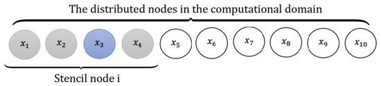
Figure 1.
Demonstration of the distributed points in the computational region with a stencil at nodal point .
The LRBF-FD computes the weighting coefficients by enforcing the requirement that the linear combination (12) must be exact for the set of RBF, , where the centers are located at
The weighting coefficients are the unknown coefficients to be computed from the above-mentioned system at every stencil [40].
2.3. Discretization of the Generalized Rosenau–Kawahara–RLW Model
The LRBF-FD method approximates the unknown function by implementing RBFs while estimating the derivative via the FD method. The major benefit of these methods is their approximation of derivatives using the FD scheme at every local support domain. As such, at each support domain, a small linear algebraic equations system must be resolved using the CPD interpolation matrix.
Here, we discretize spatial derivatives of the generalized Rosenau–Kawahara–RLW model by means of the LRBF-FD technique. Based on this, the first, third, fourth and fifth order derivatives of can be approximated by means of the function values at all nodes in the stencil of , as comes next:
where the symbol denotes the weighted differences for the order derivatives and at every stencil. The matrices structure , , , and relies on the number of nodes in every stencil. For example, if we select three nodes at every stencil, then the matrices ,, , and are tridiagonal matrices.
We obtain the following ODEs system by replacing Equations (16)–(20) in (6) and collocating nodes in it by
Here, an ODE solver is adopted for solving the system of ODEs (21) in the temporal direction. The method of lines is a method that utilizes FD in the time dimension to solve ODE problems. If all eigenvalues of the spatial discretization technique, scaled by the time step (), are within the stability region of the spatial operator approximating time, then this method is considered stable. Algorithm 1 outlines the steps for fully discretizing the 1D Rosenau–Kawahara–RLW model using this approach.
| Algorithm 1: Full discretization of the generalized Rosenau–Kawahara–RLW model |
|
3. Numerical Experiments
This section introduces three numerical examples on the generalized Rosenau–Kawahara–RLW model to measure the accuracy and the performance of the LRBF-FD technique. For this purpose, we calculate the , , and norm errors as
Here, and denote the numerical and exact solutions, respectively. The numerical examples use the multiquadric RBF (MQ) as the basis function with a shape parameter . The accuracy and flatness of the function heavily depend on this parameter , but there is no agreement on the best value. The LRBF-FD method places great importance on the selection of . To determine the optimal shape parameter , we utilize Algorithm 2 from Sarra’s method [41].
| Algorithm 2: Optimal shape parameter [41]. |
 |
The MATLAB R2016a environment on a Windows 10 desktop computer with 4 GB RAM was used for numerical computations. The condest command in MATLAB can be used to obtain the condition number (CN) of the coefficient matrix.
Example 1.
Let us study the generalized Rosenau–Kawahara–RLW model (6) associated with and on the space interval so that exact solitary wave solution is
Hereafter, we study this example based on the LRBF-FD collocation technique for different values of , N, and T. Table 1 reports the errors of numerical solutions , , and norms, CN and computational times (in seconds) at different values of stencil sizes with when . Table 2 compares the errors of numerical solutions using and norms with techniques described in [28,33] when by taking . Table 3 compares the and norm errors with methods introduced in [28,33] by various values of and N when Based on comparisons in Table 2 and Table 3, we can observe that the proposed strategy is slightly better than the techniques introduced in [28,33]. Table 4 lists the conservative invariant E over spatial interval at various total times T. It can be seen that the method is conservative perfectly (up to 5 decimals) for energy during the long-term time evolution of the solitary wave. Figure 2 shows the numerical solution and corresponding maximum norm errors when , and over spatial interval . Figure 3 displays the long-time behavior of numerical solutions with and at several total times over spatial interval . As seen in Figure 3, the single solitons move to the right-side with the preserved amplitude and shape. Finally, Figure 4 depicts the maximum norm errors at various total times with and over spatial interval .

Table 1.
Errors using , , and norms, CN and computational times with at various stencil sizes over spatial interval for Example 1 when .
Table 2.
Comparison of errors using and norms with over spatial interval for Example 1 when .
Table 3.
Errors using and norms over spatial interval for Example 1 when .
Table 4.
The conservative invariant E over spatial interval at several values of total times T for Example 1.
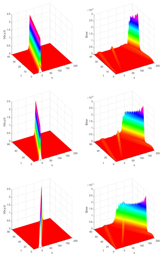
Figure 2.
The approximation solution and corresponding maximum norm errors when , and over spatial interval for Example 1.
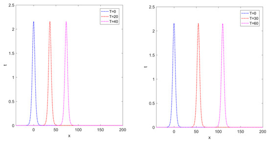
Figure 3.
The long-time behavior of approximate solutions at various total times with and over spatial interval for Example 1.
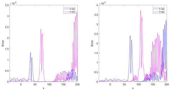
Figure 4.
The maximum norm errors at various total times with N = 350, and over spatial interval for Example 1.
Example 2.
Consider the generalized Rosenau–Kawahara–RLW model (6) associated with , and on the space interval so that the exact solitary wave solution is
This example is simulated by using the LRBF-FD collocation scheme for different values of , N, and T. Table 5 presents the errors of numerical solutions having , , and norms, CN and computational times (in seconds) at several values of stencil sizes with when . Table 6 includes the errors of approximate solutions by making use of and norms with techniques described in [28,33] by taking at total time . In view of Table 5, we can observe that the numerical accuracy of the LRBF-FD is clearly better than the technique described in [28,33]. Table 7 lists the conservative invariant E at several total times T over spatial interval . One can observe that E is conserved (up to 8 decimals) and the method can be well applied to investigate the solitary wave over a long time. Figure 5 represents the long-time behavior of numerical solutions with and at several total times over spatial interval . As observed in Figure 5, the single solitons move to the right side with the preserved amplitude and shape. Figure 6 shows the maximum norm errors at several total times with and over spatial interval . Figure 7 depicts the numerical solution and corresponding maximum norm errors when , and over spatial interval . Finally, Figure 8 depicts the relevant matrix’s sparsity structures with in the case of .
Table 5.
Errors using , , and norms, CN and computational times with at various stencil sizes over spatial interval for Example 2 when .
Table 6.
Errors using and norms with at over spatial interval for Example 2.
Table 7.
The conservative invariant E over spatial interval at various total times T for Example 2.
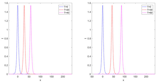
Figure 5.
The long-time behavior of numerical solutions at several total times with and over spatial interval for Example 2.
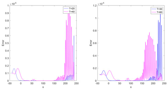
Figure 6.
The maximum norm errors at various total times with N = 1200, and over spatial interval for Example 2.
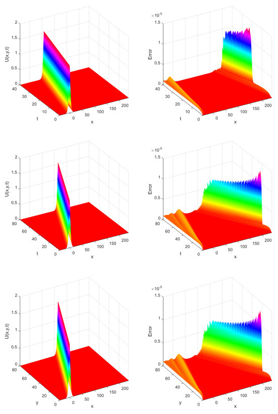
Figure 7.
The approximation solution and corresponding maximum norm errors over spatial interval for Example 2 when , and .
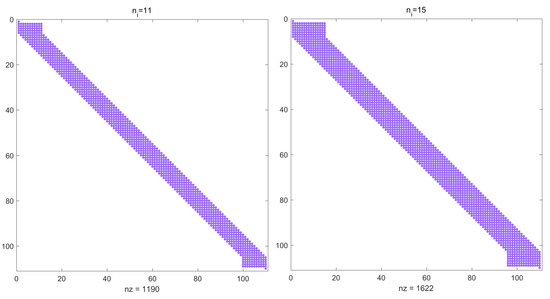
Figure 8.
The sparsity structures of the relevant matrix with for .
Example 3.
Consider the Kawahara-type Equation (6) with parameters as , and on the space interval so that the exact solitary wave solution is
The LRBF-FD collocation method is adopted for solving this problem for different values of , N, and T. Table 8 presents the errors of numerical solutions by means of , and norms, and computational times (in seconds) when at several values of stencil sizes with . Table 9 represents the errors of approximate solutions based on and norms with techniques described in [42,43] at several values of time step for , and over spatial interval In view of Table 8, we can see that the results by the proposed method show improvement over the techniques presented in [42,43]. Finally, Figure 9 depicts the numerical solution and corresponding maximum norm errors when , and over spatial interval .
Table 8.
Errors using , and norms and CPU times with when and at different stencil sizes over spatial interval for Example 3.
Table 9.
Errors using and norms at several values of time step when , , and over spatial interval for Example 3.
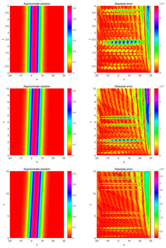
Figure 9.
The approximation solution and corresponding maximum norm errors when , and over spatial interval for Example 3.
4. Concluding Remark
This paper adopted a meshless numerical procedure for solving the IBVP of the generalized nonlinear Rosenau–Kawahara–RLW without using linearization. Firstly, the PDE was converted into a nonlinear system of ODEs through radial kernels. Afterwards, the method of lines was utilized to approximate the temporal direction and generate a system of nonlinear ODEs. Furthermore, an ODE solver was utilized to obtain highly accurate outcomes from the nonlinear ODEs system. Global RBF collocation techniques have the disadvantage of high computational cost and ill-conditioned system. The proposed method overcomes these challenges well and reduces the computational cost by sparsifying the linear system. Numerical results verified the reliability and efficiency of the present method when compared with existing ones.
Author Contributions
Conceptualization, A.A.A.-s. and O.N.; data curation, A.A.A.-s. and O.N.; formal analysis, O.N. and Z.A.; investigation, Z.A and O.N.; methodology, O.N. and Z.A.; software, O.N and Z.A.; supervision, Z.A. and A.M.L.; validation, O.N. and Z.A.; visualization, A.M.L. and O.N.; writing-original draft, Z.A. and O.N.; writing-review and editing, A.M.L. All authors have read and agreed to the published version of the manuscript.
Funding
This research received no external funding.
Data Availability Statement
No datasets were generated or analyzed during the current study.
Acknowledgments
The authors are thankful to the respected reviewers for their valuable comments and constructive suggestions towards the improvement of the original paper.
Conflicts of Interest
The authors declare no conflict of interest.
References
- Chunga, K.; Toulkeridis, T. First evidence of paleo-tsunami deposits of a major historic event in Ecuador. J. Tsunami Soc. Int. 2014, 33, 69. [Google Scholar]
- Smith, R.C.; Hill, J.; Collins, G.S.; Piggott, M.D.; Kramer, S.C.; Parkinson, S.D.; Wilson, C. Comparing approaches for numerical modelling of tsunami generation by deformable submarine slides. Ocean Model. 2016, 100, 125–140. [Google Scholar] [CrossRef]
- Sakera, S.; Hassanb, H. Asymptotic properties of solutions of third-order nonlinear dynamic equations on time scales. J. Math. Comput. Sci. 2022, 25, 255–268. [Google Scholar] [CrossRef]
- Ngondiep, E. A novel three-level time-split approach for solving two-dimensional nonlinear unsteady convection-diffusion-reaction equation. J. Math. Comput. Sci 2022, 26, 222–248. [Google Scholar] [CrossRef]
- Kumar, P.; Panwar, V. Wavelet neural network based controller design for non-affine nonlinear systems. J. Math. Comput. Sci. 2022, 24, 49–58. [Google Scholar] [CrossRef]
- Hussain, J. Exact solutions of transaction cost nonlinear models for illiq-uid markets. J. Math. Comput. Sci. 2021, 23, 263–278. [Google Scholar] [CrossRef]
- Ibrahima, A.H.; Muangchoob, K.; Mohamedc, N.S.; Abubakard, A.B. Derivative-free SMR conjugate gradient method for con-straint nonlinear equations. J. Math. Comput. Sci. 2022, 24, 147–164. [Google Scholar] [CrossRef]
- Hu, H. Dynamics of Surface Waves in Coastal Waters; Springer: Berlin/Heidelberg, Germany, 2010. [Google Scholar]
- Pedlosky, J. Waves in the Ocean and Atmosphere: Introduction to Wave Dynamics; Springer: Berlin/Heidelberg, Germany, 2003; Volume 260. [Google Scholar]
- Johnson, R.S. A Modern Introduction to the Mathematical Theory of Water Waves; Number 19; Cambridge University Press: Cambridge, UK, 1997. [Google Scholar]
- Holthuijsen, L.H. Waves in Oceanic and Coastal Waters; Cambridge University Press: Cambridge, UK, 2010. [Google Scholar]
- Barna, I.F.; Pocsai, M.A.; Mátyás, L. Time-dependent analytic solutions for water waves above sea of varying depths. Mathematics 2022, 10, 2311. [Google Scholar] [CrossRef]
- Golbabai, A.; Arabshahi, M. On the behavior of high-order compact approximations in the one-dimensional sine—Gordon equation. Phys. Scr. 2011, 83, 015015. [Google Scholar] [CrossRef]
- Molavi-Arabshahi, M.; Shavali-koohshoori, K. Application of cubic B-spline collocation method for reaction diffu-sion Fisher’s equation. Comput. Methods Differ. Equ. 2021, 9, 22–35. [Google Scholar]
- Khasi, M.; Rashidinia, J.; Rasoulizadeh, M.N. Fast Computing Approaches Based on a Bilinear Pseudo-Spectral Method for Nonlinear Acoustic Wave Equations. SIAM J. Sci. Comput. 2023, 45, B413–B439. [Google Scholar] [CrossRef]
- Khan, K.; Akbar, M.A. Solving unsteady Korteweg–de Vries equation and its two alternatives. Math. Methods Appl. Sci. 2016, 39, 2752–2760. [Google Scholar] [CrossRef]
- Rasoulizadeh, M.; Nikan, O.; Avazzadeh, Z. The impact of LRBF-FD on the solutions of the nonlinear regularized long wave equation. Math. Sci. 2021, 15, 365–376. [Google Scholar] [CrossRef]
- Demirci, A.; Hasanoğlu, Y.; Muslu, G.M.; Özemir, C. On the Rosenau equation: Lie symmetries, periodic solutions and solitary wave dynamics. Wave Motion 2022, 109, 102848. [Google Scholar] [CrossRef]
- Rosenau, P. A quasi-continuous description of a nonlinear transmission line. Phys. Scr. 1986, 34, 827. [Google Scholar] [CrossRef]
- Rosenau, P. Dynamics of dense discrete systems: High order effects. Prog. Theor. Phys. 1988, 79, 1028–1042. [Google Scholar] [CrossRef]
- Park, M. On the Rosenau equation. Mat. Appl. Comput. 1990, 9, 145–152. [Google Scholar]
- Pan, X.; Zhang, L. On the convergence of a conservative numerical scheme for the usual Rosenau-RLW equation. Appl. Math. Model. 2012, 36, 3371–3378. [Google Scholar] [CrossRef]
- Pan, X.; Zheng, K.; Zhang, L. Finite difference discretization of the Rosenau-RLW equation. Appl. Anal. 2013, 92, 2578–2589. [Google Scholar] [CrossRef]
- Atouani, N.; Omrani, K. Galerkin finite element method for the Rosenau-RLW equation. Comput. Math. Appl. 2013, 66, 289–303. [Google Scholar] [CrossRef]
- Zuo, J.M.; Zhang, Y.M.; Zhang, T.D.; Chang, F. A new conservative difference scheme for the general Rosenau-RLW equation. Bound. Value Probl. 2010, 2010, 1–13. [Google Scholar] [CrossRef]
- Pan, X.; Zhang, L. Numerical simulation for general Rosenau-RLW equation: An average linearized conservative scheme. Math. Probl. Eng. 2012, 2012, 517818. [Google Scholar] [CrossRef]
- Kawahara, T. Oscillatory solitary waves in dispersive media. J. Phys. Soc. Jpn. 1972, 33, 260–264. [Google Scholar] [CrossRef]
- He, D.; Pan, K. A linearly implicit conservative difference scheme for the generalized Rosenau–Kawahara-RLW equation. Appl. Math. Comput. 2015, 271, 323–336. [Google Scholar] [CrossRef]
- Jin, L. Application of variational iteration method and homotopy perturbation method to the modified Kawahara equation. Math. Comput. Model. 2009, 49, 573–578. [Google Scholar] [CrossRef]
- Korkmaz, A.; Dağ, İ. Crank-Nicolson–differential quadrature algorithms for the Kawahara equation. Chaos Solit. Fractals 2009, 42, 65–73. [Google Scholar] [CrossRef]
- Zuo, J.m. Soliton solutions of a general Rosenau-Kawahara-RLW equation. J. Math. Res. 2015, 7, 24. [Google Scholar] [CrossRef]
- He, D. Exact solitary solution and a three-level linearly implicit conservative finite difference method for the generalized Rosenau–Kawahara-RLW equation with generalized Novikov type perturbation. Nonlinear Dyn. 2016, 85, 479–498. [Google Scholar] [CrossRef]
- Wang, X.; Dai, W. A new implicit energy conservative difference scheme with fourth-order accuracy for the generalized Rosenau–Kawahara-RLW equation. Comput. Appl. Math. 2018, 37, 6560–6581. [Google Scholar] [CrossRef]
- Gazi Karakoc, S.B.; Kumar Bhowmik, S.; Gao, F. A numerical study using finite element method for generalized Rosenau-Kawahara-RLW equation. Comput. Methods Differ. Equ. 2019, 7, 319–333. [Google Scholar]
- Chen, W.; Fu, Z.J.; Chen, C.S. Recent Advances in Radial Basis Function Collocation Methods; Springer: Berlin/Heidelberg, Germany, 2014. [Google Scholar]
- Avazzadeh, Z.; Nikan, O.; Machado, J.A.T. Solitary wave solutions of the generalized Rosenau-KdV-RLW equation. Mathematics 2020, 8, 1601. [Google Scholar] [CrossRef]
- Nikan, O.; Avazzadeh, Z.; Machado, J.T. Numerical study of the nonlinear anomalous reaction–subdiffusion process arising in the electroanalytical chemistry. J. Comput. Sci. 2021, 53, 101394. [Google Scholar] [CrossRef]
- Nikan, O.; Avazzadeh, Z.; Rasoulizadeh, M. Soliton wave solutions of nonlinear mathematical models in elastic rods and bistable surfaces. Eng. Anal. Bound. Elem. 2022, 143, 14–27. [Google Scholar] [CrossRef]
- Nikan, O.; Avazzadeh, Z. A locally stabilized radial basis function partition of unity technique for the sine—Gordon system in nonlinear optics. Math. Comput. Simul. 2022, 199, 394–413. [Google Scholar] [CrossRef]
- Fasshauer, G.E. Meshfree Approximation Methods with MATLAB; World Scientific: Singapore, 2007; Volume 6. [Google Scholar]
- Sarra, S.A. A local radial basis function method for advection–diffusion–reaction equations on complexly shaped domains. Comput. Math. Appl. 2012, 218, 9853–9865. [Google Scholar] [CrossRef]
- Seydaoğlu, M. A meshless two-stage scheme for the fifth-order dispersive models in the science of waves on water. Ocean Eng. 2022, 250, 111014. [Google Scholar] [CrossRef]
- Rasoulizadeh, M.N.; Rashidinia, J. Numerical solution for the Kawahara equation using local RBF-FD meshless method. J. King Saud Univ. Sci. 2020, 32, 2277–2283. [Google Scholar] [CrossRef]
Disclaimer/Publisher’s Note: The statements, opinions and data contained in all publications are solely those of the individual author(s) and contributor(s) and not of MDPI and/or the editor(s). MDPI and/or the editor(s) disclaim responsibility for any injury to people or property resulting from any ideas, methods, instructions or products referred to in the content. |
© 2023 by the authors. Licensee MDPI, Basel, Switzerland. This article is an open access article distributed under the terms and conditions of the Creative Commons Attribution (CC BY) license (https://creativecommons.org/licenses/by/4.0/).