Symmetric Adaptive Higher-Order Energy-Preserving Methods for a Charged Particle System and Guiding Center System

Abstract

We propose higher-order adaptive energy-preserving methods for a charged particle system and a guiding center system. The higher-order energy-preserving methods are symmetric and are constructed by composing the second-order energy-preserving methods based on the averaged vector field. In order to overcome the energy drift problem that occurs in the energy-preserving methods based on the average vector field, we develop two adaptive algorithms for the higher-order energy-preserving methods. The two adaptive algorithms are developed based on using variable points of Gauss–Legendre’s quadrature rule and using two different stepsizes. The numerical results show that the two adaptive algorithms behave better in phase portrait and energy conservation than the Runge–Kutta methods. Moreover, it is shown that the energy errors obtained by the two adaptive algorithms can be bounded by the machine precision over long time and do not show energy drift.

1. Introduction

Any physical process in which the dissipation is negligible can in some way be represented as a Hamiltonian system. Hamiltonian systems [1,2,3,4] have the important property of having an inner symplectic structure. This property is also called area-preserving. Area-preserving means that given some pairs of canonical variable, the sum of the areas of the variable pairs is invariant across time. A canonical Hamiltonian system has the following form:

$$\dot{y}=J^{-1}\nabla H\left(y\right),y={(y_1,y_2,\cdots ,y_{2n})}^{\top }\in {\mathbb{R}}^{2n}$$

(1)

with

$$J=\left(\begin{array}{cc}0& I_n\\ -I_n& 0\end{array}\right),$$

(2)

where H is the Hamiltonian function. The symplectic structure of the canonical Hamiltonian system can be expressed in the following 2-form:

$$\omega =\sum _{k=1}^{n}d{y}_k\wedge d{y}_{n+k}.$$

(3)

For the canonical Hamiltonian system, obtaining analytical solutions is often a formidable task. Therefore, it is essential to construct numerical methods that have good properties. Numerical methods having good properties can obtain better numerical simulation [5,6] results than other methods. Thus, symplectic methods [1,7] are constructed to solve the dynamics of the Hamiltonian system. The advantage of the symplectic methods is that they exactly preserve the inner symplectic structure of the canonical Hamiltonian system. It has been shown that the symplectic methods have the near energy conservation property and long-term stability by conducting various numerical experiments in diverse disciplines, such as celestial mechanics, biology, and plasma physics [2,3,8,9,10,11]. Furthermore, symplectic methods have been found to exhibit superior long-term behavior compared to standard integrators such as explicit and implicit Runge–Kutta methods. This long-term behavior includes the near preservation of invariants without secular drift and slower error growth. Invariants that symplectic methods can effectively preserve include the Hamiltonian function, momentum, angular momentum, and others. Symplectic methods can be categorized into explicit symplectic methods and implicit ones. Explicit symplectic methods are not only effective in preserving invariants but also demonstrate better computational efficiency compared to implicit Runge–Kutta methods. Symplectic methods are applied to the Kepler problem [12,13], the restricted three-body problem [14,15], and the charged particle system [10,11], and they are compared with other numerical methods. Symplectic methods that are a generalization of the commutator-free quasi-Magnus exponential integrators were built for the Kepler problem, and they are shown to be more efficient than the Runge-Kutta methods [12]. A family of adaptive symplectic conservative numerical methods for the Kepler problem were constructed, and the methods preserved all the global properties of the exact solution of the problem [13]. The force gradient symplectic methods were constructed for the circular restricted three-body problem, and the numerical results showed that the fourth-order force gradient symplectic method always exhibits better numerical accuracy than the non-gradient Forest–Ruth algorithm [14]. Symplectic algorithms for solving the restricted three-body problem were constructed, and their advantages have been shown in phase portrait and energy conservation compared with the fourth-order Runge–Kutta method [15]. Explicit symplectic methods were constructed for the non-relativistic and relativistic charged particle dynamics, and the numerical results showed that the symplectic methods behave better in long-term energy conservation and numerical efficiency than the Runge–Kutta methods [10,11]. Blanes and Moan developed several higher-order symplectic methods using the splitting method for the Hamiltonian system, and these methods had higher precision than the Runge–Kutta methods [16]. A non-canonical Hamiltonian system [2,9,17,18] is the generalization of a canonical Hamiltonian system. Many systems, including the Lotka–Volterra model [2], the nonlinear Schrödinger equation [19,20], and the guiding center system [17,21], can be expressed as non-canonical Hamiltonian systems. They have the same form as canonical Hamiltonian systems, where the matrix J is represented by a skew-symmetric matrix $K^{-1}\left(y\right)$ which depends on the variable y. The non-canonical Hamiltonian system also possesses a K-symplectic structure which is exactly preserved by the K-symplectic method [22,23,24]. Explicit K-symplectic methods have been widely constructed for non-canonical Hamiltonian systems [22,24,25]. Explicit K-symplectic methods are constructed using the splitting method for the charged particle system, and the numerical results showed that they behave better in phase portrait than the Runge–Kutta method and they are more stable than the Boris method in numerical calculation [22]. Explicit K-symplectic methods were constructed for the bright and dark soliton motion of the nonlinear Schrödinger equation, and they were found to be more efficient than the canonical symplectic methods [24,25].

Symplectic and K-symplectic methods belong to a class of structure-preserving methods which aim to maintain the inherit structure of a system throughout numerical simulations. The other notable structure-preserving methods encompass the energy-preserving methods [26,27,28] and the volume-preserving methods [29,30,31]. Volume-preserving methods are tailored for source-free systems, where their volumes remain invariant over time, ensuring the preservation of system volume. On the other hand, energy-preserving methods are usually constructed for canonical and non-canonical Hamiltonian systems. In contrast to conventional numerical approaches, which can suffer from energy dissipation issues, energy-preserving methods offer a numerical solution that exactly preserves the system’s energy. This enhancement is crucial in ensuring the reliability of simulation results. For example, standard Runge–Kutta methods are prone to energy dissipation, leading to inaccuracies in phase portraits [10,11,22]. Therefore, the development of energy-preserving methods addresses this challenge and enables the exact preservation of energy. Consequently, the application of energy-preserving methods extends to any system possessing invariants—quantities that remain constant over time. The Hamiltonian function of the both canonical and non-canonical Hamiltonian system is one invariant of the corresponding system. The Hamiltonian function is also called the energy of the system. Energy-preserving methods exactly preserve the Hamiltonian function of the system. There are several approaches to constructing energy-preserving methods, such as the discrete gradient method [32], the averaged vector field method [33,34], the line integral method [26,35], the projection method [2], and so on. Recently, energy-preserving methods were constructed for charged particle systems [35,36,37,38,39] and guiding center systems [17,18,40]. Both charged particle systems [10,11,23] and the guiding center systems [17,21] can be expressed as non-canonical Hamiltonian systems. Thus, energy-preserving methods are developed for these two systems. Li and Wang constructed a second-order energy-preserving method using the discrete line integral method for the charged particle system [36]. The Boris method is a well-known symmetric numerical method for the charged particle system. It is shown that the discrete line method behaves better in energy conservation than the Boris method [36]. Within the framework of the line integral method, Brugnano et al. constructed higher-order energy-preserving methods using orthogonal polynomials and quadrature rules [35] for a charged particle system. The numerical results show that the higher-order energy-preserving methods exhibit much better energy conservation than the Boris method and implicit midpoint method, and they are also more effective than the Boris method [35]. Li and Wang constructed several efficient energy-preserving methods for charged particle systems [38,39]. The energy errors of energy-preserving methods are much smaller than the Boris method [38,39]. Zhang et al. constructed energy-preserving methods based on the Ito–Abe discrete gradient for guiding center systems [40]. Zhu et al. constructed a family of energy-preserving methods for guiding center systems based on the averaged vector field [17,18]. The energy-preserving methods are shown to have excellent energy conservation behavior [17,18].

A family of energy-preserving methods has been constructed for guiding center systems; however, these methods based on the averaged vector field exhibit an energy drift over a long time [17]. We aim to construct adaptive higher-order energy-preserving methods based on the averaged vector field that can overcome the energy drift problem. The higher-order energy-preserving methods are constructed by composing the second-order energy-preserving methods proposed in Reference [17]. Thus, we can obtain a family of fourth-order and sixth-order energy-preserving methods. The higher-order energy-preserving methods can have higher numerical accuracy which means that the error in the variable is smaller than the lower-order methods. However, since the second-order energy-preserving methods exhibit energy drift, it is expected that the higher-order methods composed of these second-order methods will also display the same issue. In order to overcome the energy drift problem, for the higher order energy-preserving methods based on composition, we provide two adaptive strategies and develop two adaptive algorithms. The main idea of the first adaptive algorithm is to increase the number of points of the Guass Legendre’s quadrature rule used in the energy-preserving methods if the energy error is larger than the tolerance error. And if we use three different points of the Gaussian quadrature, the energy errors are all larger than the tolerance error, then we prefer the Gaussian quadrature with least error. The idea of the second-order adaptive algorithms is to use two different time stepsizes (h and $1.05h$) for the same energy-preserving method, and we choose the stepsize with smaller error. To evaluate the effectiveness of the adaptive algorithms, we compare them with standard Runge–Kutta methods and energy-preserving methods that do not employ any adaptive strategies. The numerical results show that the two adaptive algorithms do not show energy drifts, and their energy errors can be bounded to the machine’s precision.

The rest of the paper is organized as follows. Section 2 gives a brief introduction to the non-canonical Hamiltonian system, the charged particle system, and the guiding center system. Section 3 presents how higher-order energy-preserving methods are constructed by using the composing method. In Section 4, we give a detailed description on the two adaptive algorithms. The implementation of the two algorithms is also presented. In Section 5, numerical results of the charged particle system and the guiding center system are provided. The two adaptive algorithms are compared with the standard Runge–Kutta methods and the energy-preserving methods without using any adaptive strategy. In Section 6, we summarize our work.

2. Charged Particle System and Guiding Center System

2.1. Non-Canonical Hamiltonian System

Both the charged particle system and the guiding center system are fundamental systems in plasma physics, and they can be written as non-canonical Hamiltonian systems [2,9,17,18]. The non-canonical Hamiltonian systems can be expressed as the following differential equation:

$$\dot{Z}=K^{-1}\left(Z\right)\nabla H\left(Z\right)Z\in {\mathbb{R}}^{2n},$$

(4)

where $H\left(Z\right)$ is the Hamiltonian function and ∇ is the gradient operator. Different from a canonical Hamiltonian system, a non-canonical Hamiltonian system has a more general form. In a non-canonical Hamiltonian system (4), $K^{-1}\left(Z\right)$ is a skew-symmetric matrix which depends on the variable Z while in a canonical Hamiltonian system, $K^{-1}\left(Z\right)$ is replaced by a constant matrix

$$J=\left(\begin{array}{cc}0& I_n\\ -I_n& 0\end{array}\right).$$

(5)

Meanwhile, $K\left(Z\right)$ satisfies the Jacobi identity

$$\frac{\partial k_{ij}}{\partial z_k}+\frac{\partial k_{jk}}{\partial z_i}+\frac{\partial k_{ki}}{\partial z_j}=0,1\le i,j,k\le 2n,$$

(6)

where $k_{ij}$ is the element in the i-th row and the j-th column of the matrix $K\left(Z\right)$ for any $i,j=1,2,\dots ,2n$ and $z_k$ is the k-th component of Z for any $k=1,2,\dots ,2n$.

Assume that the exact phase flow (analytical solution) of the non-canonical Hamiltonian system is ${\varphi }_t\left(Z\right)$; then, we know that the Hamiltonian function $H\left(Z\right)$ is exactly preserved by the phase flow ${\varphi }_t\left(Z\right)$, i.e.,

$$\begin{array}{ccc}& & \frac{dH\left({\varphi }_t\left(Z\right)\right)}{dt}=\frac{\partial H\left({\varphi }_t\left(Z\right)\right)}{\partial {\varphi }_t\left(Z\right)}\frac{d{\varphi }_t\left(Z\right)}{dt}=\frac{\partial H\left({\varphi }_t\left(Z\right)\right)}{\partial {\varphi }_t\left(Z\right)}{K}^{-1}\left({\varphi }_t\left(Z\right)\right)\nabla H\left({\varphi }_t\left(Z\right)\right)\hfill \end{array}$$

(7)

$$\begin{array}{ccc}& =& {(\nabla H\left({\varphi }_t\left(Z\right)\right))}^{\top }{K}^{-1}\left({\varphi }_t\left(Z\right)\right)\nabla H\left({\varphi }_t\left(Z\right)\right)=0,\hfill \end{array}$$

(8)

the last equality holds because the matrix $K^{-1}$ is skew-symmetric. Thus, we derive that $H\left({\varphi }_t\left(Z\right)\right)=H\left({\varphi }_0\left(Z\right)\right)=H\left(Z_0\right)$, where $Z_0$ is the initial value of the variable Z. This means that the Hamiltonian function H is invariant along time t, i.e., H is a conservation law.

It is often difficult to obtain the analytical solution of a non-canonical Hamiltonian system. Thus, the role of the numerical methods becomes increasingly important. Among them, structure-preserving methods play an important role in the numerical calculations of non-canonical Hamiltonian systems due to their structure-preserving properties and long-term stability. As the Hamiltonian function H is an invariant, we can construct the numerical methods that exactly preserve H. The Hamiltonian function H is also called the energy of the system. This kind of numerical method is called an energy-preserving method [26,27,28,32,33,38].

Definition 1.

A numerical method ${\mathsf{\Phi }}_h:Z_n\to Z_{n+1}$ is a one-step method where h is the time stepsize. Assume that the value $Z\in {\mathbb{R}}^{2n}$ at the initial time $t_0$ is $Z_0$. Using the numerical method ${\mathsf{\Phi }}_h$, we can obtain the values of Z at a series of time steps $t_0+nh$, i.e., $Z_n={\mathsf{\Phi }}_h\left(Z_{n-1}\right),n=1,2,\cdots$. The method is called an energy-preserving method if

$$H\left(Z_n\right)=H\left({\mathsf{\Phi }}_h\left(Z_{n-1}\right)\right)=H\left(Z_{n-1}\right),$$

(9)

that is to say, the energy H is exactly preserved [27,41].

If we have two energy-preserving methods, then the method composed by the two methods is also an energy-preserving method.

Theorem 1.

If both ${\mathsf{\Phi }}_h$ and ${\mathsf{\Psi }}_h$ are energy-preserving methods, then ${\mathsf{\Phi }}_{h/2}\circ {\mathsf{\Psi }}_{h/2}$ is also an energy-preserving method [17].

Remark 1.

Theorem 1 also applies for the composition of several energy-preserving methods.

We can construct higher-order energy-preserving methods based on composition for charged particle systems and guiding center systems.

2.2. Charged Particle Systems

The charged particle system written in the variable ($\mathbf{X}$, $\mathbf{V}$) is the following differential equation:

$$\frac{d\mathbf{X}}{dt}=\mathbf{V},m\frac{d\mathbf{V}}{dt}=q(E\left(\mathbf{X}\right)+\mathbf{V}\times B\left(\mathbf{X}\right)),$$

(10)

where $\mathbf{X}=(x_1,x_2,x_3)$ is the position of the particle and $\mathbf{V}=(v_1,v_2,v_3)$ is the velocity of the particle, $E\left(\mathbf{X}\right)$ is the electric field, and $B\left(\mathbf{X}\right)$ is the magnetic field. In the system (10), the mass of the particle is m and the charge is q. If we combine the two components of the variable as $Z={(\mathbf{X},\mathbf{V})}^{\top }$, then the charged particle system can be written as a non-canonical Hamiltonian system (4) with the Hamiltonian function being $H(\mathbf{X},\mathbf{V})=m{v}_1^2/2+m{v}_2^2/2+m{v}_3^2/2+q\phi \left(\mathbf{X}\right)$. Here, the skew-symmetric matrix is of the form

$$K^{-1}\left(Z\right)=\left(\begin{array}{cc}O& \frac{I}{m}\\ -\frac{I}{m}& -\frac{q\widehat{B}\left(\mathbf{X}\right)}{m^2}\end{array}\right)$$

(11)

with I being the $3\times 3$ identity matrix. The relationship between the scalar potential $\phi \left(\mathbf{X}\right)$ and the electric field is $E\left(\mathbf{X}\right)=-\nabla \phi$. The magnetic field is composed as $B\left(\mathbf{X}\right)=(B_1\left(\mathbf{X}\right),B_2\left(\mathbf{X}\right),B_3\left(\mathbf{X}\right))$, and the matrix $\widehat{B}\left(\mathbf{X}\right)$ in the matrix $K^{-1}\left(\mathbf{Z}\right)$ is

$$\widehat{B}\left(\mathbf{X}\right)=\left(\begin{array}{ccc}0& -B_3\left(\mathbf{X}\right)& B_2\left(\mathbf{X}\right)\\ B_3\left(\mathbf{X}\right)& 0& -B_1\left(\mathbf{X}\right)\\ -B_2\left(\mathbf{X}\right)& B_1\left(\mathbf{X}\right)& 0\end{array}\right).$$

(12)

The magnetic field satisfies the divergence-free property $\nabla ·B\left(\mathbf{X}\right)=0$. Then, we know that a vector potential $A\left(\mathbf{X}\right)$ exists such that $B\left(\mathbf{X}\right)=\nabla \times A\left(\mathbf{X}\right)$.

The charged particle system is a multi-timescale problem, as its motion has two components: the fast gyromotion and the slow guiding center motion. In order to deal with the tough multi-scale problem, the gyrokinetic and related theories emerge as a branch of magnetized plasmas. The motion of the guiding center can be derived by averaging out the fast gyromotion from the charged particle motion and the corresponding behavior of the guiding center is governed by the theory of gyrokinetics.

2.3. Guiding Center Systems

Littlejohn first gave the Lagrangian of the guiding center system as [42]

$$L(\mathbf{X},\dot{\mathbf{X}},u,\dot{u})=[\mathbf{A}\left(\mathbf{X}\right)+u\mathbf{b}\left(\mathbf{X}\right)]·\dot{\mathbf{X}}-\left[\frac{1}{2}{u}^2+\mu B\left(\mathbf{X}\right)+\phi \left(\mathbf{X}\right)\right].$$

(13)

The Euler–Lagrange equations of the Lagrangian L with respect to the position of the guiding center $\mathbf{X}$ and the parallel velocity of the guiding center u result in the guiding center motion [17,21,42], which can also be expressed as a non-canonical Hamiltonian system

$$\dot{Z}=K^{-1}\left(Z\right)\nabla H\left(Z\right),Z={({\mathbf{X}}^{\top },u)}^{\top }={(x,y,z,u)}^{\top }$$

(14)

with the skew-symmetric matrix being

$$K^{-1}\left(Z\right)=\frac{1}{\sqrt{{\left|a_{23}{b}_1-a_{13}{b}_2+a_{12}{b}_3\right|}^2}}\left(\begin{array}{cccc}0& -b_3& b_2& a_{23}\\ b_3& 0& -b_1& -a_{13}\\ -b_2& b_1& 0& a_{12}\\ -a_{23}& a_{13}& -a_{12}& 0\end{array}\right).$$

(15)

The elements in the matrix $K^{-1}\left(\mathbf{Z}\right)$ are as follows:

$$\begin{array}{ccc}\hfill a_{12}& =& (\frac{\partial A_2}{\partial x}-\frac{\partial A_1}{\partial y})+u(\frac{\partial b_2}{\partial x}-\frac{\partial b_1}{\partial y}),\hfill \end{array}$$

(16)

$$\begin{array}{ccc}\hfill a_{13}& =& (\frac{\partial A_3}{\partial x}-\frac{\partial A_1}{\partial z})+u(\frac{\partial b_3}{\partial x}-\frac{\partial b_1}{\partial z}),\hfill \end{array}$$

(17)

$$\begin{array}{ccc}\hfill a_{23}& =& (\frac{\partial A_3}{\partial y}-\frac{\partial A_2}{\partial z})+u(\frac{\partial b_3}{\partial y}-\frac{\partial b_2}{\partial z}).\hfill \end{array}$$

(18)

The Hamiltonian function of the non-canonical Hamiltonian system (14) is $H\left(Z\right)=\frac{1}{2}{u}^2+\mu B\left(\mathbf{X}\right)+\phi \left(\mathbf{X}\right)$. Here, the function $\phi \left(\mathbf{X}\right)$ is the scalar potential and $\mu$ is the magnetic moment. Given a vector potential $\mathbf{A}\left(\mathbf{X}\right)=(A_1\left(\mathbf{X}\right),A_2\left(\mathbf{X}\right),A_3\left(\mathbf{X}\right))$, we can obtain the magnetic filed as $\mathbf{B}\left(\mathbf{X}\right)=\nabla \times \mathbf{A}$. The strength of the magnetic field is $B\left(\mathbf{X}\right)=\left|\mathbf{B}\right|$, and the unit vector along the direction of the magnetic field is $\mathbf{b}\left(\mathbf{X}\right)=(b_1\left(\mathbf{X}\right),b_2\left(\mathbf{X}\right),b_3\left(\mathbf{X}\right))=\mathbf{B}\left(\mathbf{X}\right)/B\left(\mathbf{X}\right)$.

3. High-Order Symmetric Energy-Preserving Methods

We consider a family of energy-preserving methods

$$Z_{n+1}=Z_n+h{K}^{-1}(\lambda Z_n+(1-\lambda )Z_{n+1}){\int }_0^1\nabla H((1-\tau )Z_n+\tau Z_{n+1})d\tau$$

(19)

based on the averaged vector field [33,34], where the parameter $\lambda \in [0,1]$. We denote the above methods by ${\mathsf{\Phi }}_{\lambda ;h},\lambda \in [0,1]$. When $\lambda =\frac{1}{2}$, the method is of order 2; otherwise, the other methods are of order 1. In order to obtain a higher-order method, we can use the composition method. Take the method ${\mathsf{\Phi }}_{{\lambda }_1;h}$ with a certain value ${\lambda }_1$ as an example; we can compose it with its adjoint method ${\mathsf{\Phi }}_{{\lambda }_1;h}^{\ast }$ to obtain a second-order method.

Definition 2.

The adjoint method ${\mathsf{\Phi }}_{{\lambda }_1;h}^{\ast }$ is the inverse of the method ${\mathsf{\Phi }}_{{\lambda }_1;h}$ with reversed time step $-h$ [2], that is,

$${\mathsf{\Phi }}_{{\lambda }_1;h}^{\ast }:={\mathsf{\Phi }}_{{\lambda }_1;-h}^{-1}.$$

(20)

If a method ${\mathsf{\Psi }}_h$ satisfies ${\mathsf{\Psi }}_h^{\ast }={\mathsf{\Psi }}_h$, then the method is called a symmetric method. In order to obtain the adjoint method of ${\mathsf{\Phi }}_{{\lambda }_1;h}$, we make the following changes in the method ${\mathsf{\Phi }}_{{\lambda }_1;h}$,

$$Z_n\leftrightarrow Z_{n+1},h\leftrightarrow -h,$$

(21)

and this results in

$$Z_n=Z_{n+1}-h{K}^{-1}({\lambda }_1{Z}_{n+1}+(1-{\lambda }_1)Z_n){\int }_0^1\nabla H((1-\tau )Z_{n+1}+\tau Z_n)d\tau .$$

(22)

Performing a variable transformation $\eta =1-\tau$, then we obtain

$$Z_n=Z_{n+1}-h{K}^{-1}((1-{\lambda }_1)Z_n+{\lambda }_1{Z}_{n+1}){\int }_0^1\nabla H((1-\eta )Z_n+\eta Z_{n+1})d\eta .$$

(23)

Then by removing the last term of the right-hand side of the equation to the left, this results in

$$Z_{n+1}=Z_n+h{K}^{-1}((1-{\lambda }_1)Z_n+{\lambda }_1{Z}_{n+1}){\int }_0^1\nabla H((1-\eta )Z_n+\eta Z_{n+1})d\eta .$$

(24)

This method is exactly ${\mathsf{\Phi }}_{1-{\lambda }_1;h}$. Thus, the adjoint method of the method ${\mathsf{\Phi }}_{{\lambda }_1;h}$ is ${\mathsf{\Phi }}_{1-{\lambda }_1;h}$, i.e., ${\left({\mathsf{\Phi }}_{{\lambda }_1;h}\right)}^{\ast }={\mathsf{\Phi }}_{1-{\lambda }_1;h}$. Therefore, we can obtain a second-order method based on the composition

$${\mathsf{\Phi }}_{{\lambda }_1,h}^2\equiv {\mathsf{\Phi }}_{1-{\lambda }_1;h/2}\circ {\mathsf{\Phi }}_{{\lambda }_1;h/2},$$

(25)

where the operation ∘ means composite mapping. According to Theorem 1, the method ${\mathsf{\Phi }}_{{\lambda }_1,h}^2$ is a second-order energy-preserving method. Then, we know that ${\mathsf{\Phi }}_{{\lambda }_1,h}^2:Z_n\to Z_{n+1}$ is

$$Z_{n+1/2}=Z_n+\frac{1}{2}h{K}^{-1}({\lambda }_1{Z}_n+(1-{\lambda }_1)Z_{n+1/2}){\int }_0^1\nabla H((1-\tau )Z_n+\tau Z_{n+1/2})d\tau ,$$

(26)

$$Z_{n+1}=Z_{n+1/2}+\frac{1}{2}h{K}^{-1}((1-{\lambda }_1)Z_{n+1/2}+{\lambda }_1{Z}_{n+1}){\int }_0^1\nabla H((1-\tau )Z_{n+1/2}+\tau Z_{n+1})d\tau .$$

(27)

It can be easily proven that ${\left({\mathsf{\Phi }}_{{\lambda }_1,h}^2\right)}^{\ast }={\mathsf{\Phi }}_{{\lambda }_1,h}^2$; thus, it is symmetric. Therefore, ${\mathsf{\Phi }}_{{\lambda }_1,h}^2$ is a second-order symmetric energy-preserving method.

In the same way, we can compose higher-order methods based on the second-order energy-preserving method ${\mathsf{\Phi }}_{{\lambda }_1;h}^2$. By using Yoshida’s method [43], we can construct a fourth-order symmetric method

$${\mathsf{\Phi }}_{{\lambda }_1;h}^4\equiv {\mathsf{\Phi }}_{{\lambda }_1;{\alpha }_{1}h}^2\circ {\mathsf{\Phi }}_{{\lambda }_1;{\beta }_{1}h}^2\circ {\mathsf{\Phi }}_{{\lambda }_1;{\alpha }_{1}h}^2,$$

(28)

where ${\alpha }_1={(2-2^{1/3})}^{-1}$ and ${\beta }_1=1-2{\alpha }_1$. According to Remark 1, the method ${\mathsf{\Phi }}_{{\lambda }_1,h}^4$ is a fourth-order symmetric energy-preserving method. More specifically, we can express the fourth-order symmetric energy-preserving method ${\mathsf{\Phi }}_{{\lambda }_1;h}^4:Z_n\to Z_{n+1}$ as follows:

$$u=Z_n+\frac{1}{2}{\alpha }_{1}h{K}^{-1}({\lambda }_1{Z}_n+(1-{\lambda }_1)u){\int }_0^1\nabla H((1-\tau )Z_n+\tau u)d\tau ,$$

(29)

$$\tilde{u}=u+\frac{1}{2}{\alpha }_{1}h{K}^{-1}((1-{\lambda }_1)u+{\lambda }_1\tilde{u}){\int }_0^1\nabla H((1-\tau )u+\tau \tilde{u})d\tau ,$$

(30)

$$v=\tilde{u}+\frac{1}{2}{\beta }_{1}h{K}^{-1}({\lambda }_1\tilde{u}+(1-{\lambda }_1)v){\int }_0^1\nabla H((1-\tau )\tilde{u}+\tau v)d\tau ,$$

(31)

$$\tilde{v}=v+\frac{1}{2}{\beta }_{1}h{K}^{-1}((1-{\lambda }_1)v+{\lambda }_1\tilde{v}){\int }_0^1\nabla H((1-\tau )v+\tau \tilde{v})d\tau ,$$

(32)

$$w=\tilde{v}+\frac{1}{2}{\alpha }_{1}h{K}^{-1}({\lambda }_1\tilde{v}+(1-{\lambda }_1)w){\int }_0^1\nabla H((1-\tau )\tilde{v}+\tau w)d\tau ,$$

(33)

$$Z_{n+1}=w+\frac{1}{2}{\alpha }_{1}h{K}^{-1}((1-{\lambda }_1)w+{\lambda }_1{Z}_{n+1}){\int }_0^1\nabla H((1-\tau )w+\tau Z_{n+1})d\tau .$$

(34)

Meanwhile, we can also compose a sixth-order symmetric energy-preserving method based on the fourth-order method ${\mathsf{\Phi }}_{{\lambda }_1;h}^4$ by using Yoshida’s method [43], i.e.,

$${\mathsf{\Phi }}_{{\lambda }_1;h}^6\equiv {\mathsf{\Phi }}_{{\lambda }_1;{\alpha }_{2}h}^4\circ {\mathsf{\Phi }}_{{\lambda }_1;{\beta }_{2}h}^4\circ {\mathsf{\Phi }}_{{\lambda }_1;{\alpha }_{2}h}^4,$$

(35)

where ${\alpha }_2={(2-2^{1/5})}^{-1}$ and ${\beta }_2=1-2{\alpha }_2$. As $\lambda$ can be any real number in $[0,1]$, we thus obtain a family of fourth-order and sixth-order symmetric energy-preserving methods.

As can be seen, there is an integral whose format is similar to ${\int }_0^1\nabla H((1-\tau )Z_n+\tau Z_{n+1})d\tau$ in each method. If the gradient of the Hamiltonian function cannot be exactly integrated, then we need to use the quadrature rule to approximate it. One of the commonly used quadrature rules is the Gauss–Legendre’s quadrature rule because it has a high-order degree of precision. We can use the Gauss–Legendre’s quadrature rule to approximate ${\int }_0^1\nabla H((1-\tau )Z_n+\tau Z_{n+1})d\tau$ under the transformation $\sigma =2\tau -1$. Then, we obtain

$$\begin{array}{ccc}& & {\int }_0^1\nabla H((1-\tau )Z_n+\tau Z_{n+1})d\tau ={\int }_{-1}^1\frac{1}{2}\nabla H\left(Z_n+\frac{1+\sigma }{2}(Z_{n+1}-Z_n)\right)d\sigma \hfill \end{array}$$

(36)

$$\begin{array}{ccc}& \approx & \frac{1}{2}\sum _{i=1}^n{\omega }_i\nabla H\left(Z_n+\frac{1+x_i}{2}(Z_{n+1}-Z_n)\right),\hfill \end{array}$$

(37)

where ${\omega }_i$ are the weights of the Legendre polynomial of degree n and $x_i$ are the corresponding nodes. Let $(w_i,c_i),1\le i\le s$ be the pair of the ith weight and node of the s-point Gauss–Legendre’s quadrature rule on $[0,1]$. Then, the method ${\mathsf{\Phi }}_{{\lambda }_1;h}$ takes the following form:

$$Z_{n+1}=Z_n+h{K}^{-1}(\lambda Z_n+(1-\lambda )Z_{n+1})\sum _{i=1}^s{w}_i\nabla H(Z_n+c_i(Z_{n+1}-Z_n)).$$

(38)

The number of the points in the Gauss–Legendre’s quadrature rule can be chosen arbitrarily. In general, if we choose more points of the Gauss–Legendre’s quadrature, we will obtain a higher precision.

4. Two Adaptive Algorithms Based on Higher-Order Energy-Preserving Methods

As is shown in Reference [17], the quadrature error caused by using the fixed s-point Gauss–Legendre’s quadrature rule, the error from the nonlinear solver, and the round-off error of the machine are the main reasons causing a numerical drift of the Hamiltonian function (the energy of the system). More specifically, we take the method ${\mathsf{\Phi }}_{{\lambda }_1;h}$ as an example. Thus, the nonlinear solver takes the following form:

$$Z_{n+1}=Z_n+h{K}^{-1}(\lambda Z_n+(1-\lambda )Z_{n+1})\sum _{i=1}^s{w}_i\nabla H(Z_n+c_i(Z_{n+1}-Z_n)).$$

(39)

So there will be points $Z_n$ and $Z_{n+1}$ that exactly satisfy

$$Z_{n+1}-Z_n=h{K}^{-1}(\lambda Z_n+(1-\lambda )Z_{n+1})\sum _{i=1}^s{w}_i\nabla H(Z_n+c_i(Z_{n+1}-Z_n))+er{r}_{S,n}$$

(40)

with $er{r}_{S,n}$ being the error from the nonlinear solver. Then, we assume that the quadrature rule approximates the integral as

$${\int }_0^1\nabla H((1-\tau )Z_n+\tau Z_{n+1})d\tau =\sum _{i=1}^s{w}_i\nabla H(Z_n+c_i(Z_{n+1}-Z_n))+er{r}_{Q,n},$$

(41)

where $er{r}_{Q,n}$ is the error caused by the quadrature rule.

Let

$$Err={\left({\int }_0^1\nabla H((1-\tau )Z_n+\tau Z_{n+1})d\tau \right)}^{\top }(Z_{n+1}-Z_n)$$

(42)

Then, we have

$$\begin{array}{ccc}& & Err={\left({\int }_0^1\nabla H((1-\tau )Z_n+\tau Z_{n+1})d\tau \right)}^{\top }(Z_{n+1}-Z_n)\hfill \\ \hfill & =& {\int }_0^1\frac{d}{d\tau }H((1-\tau )Z_n+\tau Z_{n+1})d\tau =H\left(Z_{n+1}\right)-H\left(Z_n\right).\hfill \end{array}$$

(43)

Furthermore, by substituting Equations (40) and (41), we have

$$\begin{array}{ccc}\hfill & & H\left(Z_{n+1}\right)-H\left(Z_n\right)={\left({\int }_0^1\nabla H((1-\tau )Z_n+\tau Z_{n+1})d\tau \right)}^{\top }(Z_{n+1}-Z_n)\hfill \\ & =& {\left(\sum _{i=1}^s{w}_i\nabla H(Z_n+c_i(Z_{n+1}-Z_n))+er{r}_{Q,n}\right)}^{\top }(h{K}^{-1}(\lambda Z_n+(1-\lambda )Z_{n+1})\hfill \\ \hfill & & ·\sum _{i=1}^s{w}_i\nabla H(Z_n+c_i(Z_{n+1}-Z_n)+er{r}_{S,n}).\hfill \end{array}$$

(44)

Let $G_n={\sum }_{i=1}^s{w}_i\nabla H(Z_n+c_i(Z_{n+1}-Z_n))$; then, we have

$$\begin{array}{ccc}& & H\left(Z_{n+1}\right)-H\left(Z_n\right)=h{\left(G_n\right)}^{\top }{K}^{-1}(\lambda Z_n+(1-\lambda )Z_{n+1})G_n+{\left(G_n\right)}^{\top }er{r}_{S,n}\hfill \\ \hfill & & +h{\left(er{r}_{Q,n}\right)}^{\top }{K}^{-1}(\lambda Z_n+(1-\lambda )Z_{n+1})G_n+{\left(er{r}_{Q,n}\right)}^{\top }er{r}_{S,n}.\hfill \end{array}$$

(45)

The first term on the right-hand side of the above equation ${\left(G_n\right)}^{\top }{K}^{-1}(\lambda Z_n+(1-\lambda )Z_{n+1})G_n$ vanishes because the matrix $K^{-1}$ is skew-symmetric. Therefore, the difference in the Hamiltonian function between the adjacent time steps is

$$\begin{array}{ccc}& & H\left(Z_{n+1}\right)-H\left(Z_n\right)={\left(G_n\right)}^{\top }er{r}_{S,n}+h{\left(er{r}_{Q,n}\right)}^{\top }{K}^{-1}(\lambda Z_n+(1-\lambda )Z_{n+1})G_n\hfill \\ \hfill & & +{\left(er{r}_{Q,n}\right)}^{\top }er{r}_{S,n}.\hfill \end{array}$$

(46)

The three terms in the above equation depict the error from the nonlinear solver and the error from the quadrature rule for the Hamiltonian function H after one time step. The round-off error should also be considered in the implementation of the numerical method ${\mathsf{\Phi }}_{{\lambda }_1;h}$. For only one time step, the quadrature error $er{r}_{Q,n}$ and the error from the nonlinear solver $er{r}_{S,n}$ together with the round-off error are all very small and can be neglected. But when the total number of time steps is very large, the three sources of errors may accumulate, and as a result, it may cause numerical drift in the Hamiltonian function.

It is pointed out in Reference [17] that second-order energy-preserving methods cause numerical drifts in the energy. Higher-order energy-preserving methods are composed of second-order energy-preserving methods. The higher-order methods need more composition time. Thus, energy drift will also occur in higher-order energy-preserving methods. To overcome the energy drift problem, we aim at constructing two adaptive algorithms for the higher-order energy-preserving methods. Taking the fourth-order energy-preserving methods ${\mathsf{\Phi }}_{{\lambda }_1;h}^4$ or the sixth-order methods ${\mathsf{\Phi }}_{{\lambda }_1;h}^6$ as examples, we construct two adaptive algorithms based on varying the number of points in Gauss–Legendre’s quadrature rule and varying the time stepsize. By varying the number of points used in Gauss-Legendre’s quadrature rule and choosing two different stepsizes, the energy errors may be bounded and do not show numerical drifts. This will be clearly shown in the numerical experiments part.

4.1. Algorithm 1

We give a detailed description of Algorithm 1. Algorithm 1 can be used to compute the value of $Z_{n+1}$ at each time step based on the method ${\mathsf{\Phi }}_{{\lambda }_1;h}^4$ or ${\mathsf{\Phi }}_{{\lambda }_1;h}^6$. Here, $Z_0$ is the value at initial time step, and $Z_{n+1}$ is calculated based on $Z_n$ at its former time step. We set a tolerance error $del$ to control the energy error. Firstly, we choose the number of points used in Gauss–Legendre’s quadrature rule to be $k=5$. We calculate $Z_{n+1}^k$ based on the method ${\mathsf{\Phi }}_{{\lambda }_1;h}^4$ or ${\mathsf{\Phi }}_{{\lambda }_1;h}^6$ using the k-point Gauss–Legendre quadrature. Then, we compute the energy error between the $n+1$-th time step and the initial step $tol=H\left(Z_{n+1}^k\right)-H\left(Z_0\right)$. If $tol$ is smaller than the tolerance error $del$, then we stop the algorithm. If $tol$ is larger than $del$, then we increase the number of points, and compute $Z_{n+1}^{k+1}$ using the $k+1$-point Gaussian quadrature. The algorithm stops when the updated $tol$ is less than $del$. If k reaches 8 and the updated $tol$ is still larger than the tolerance error, then we store all the energy errors calculated by the five-point, six-point, and seven-point Gaussian quadrature rules and choose the one that has the smallest error. The value of $Z_{n+1}$, which has the smallest energy error will be the final value of the algorithm. By using this adaptive algorithm, we can make sure that the energy error between the current time step and the initial step is less than the tolerance error or is the smallest among the three Gaussian quadratures we use. The tolerance error $del$ is not fixed and is used as an input. The tolerance error $del$ can sometimes be used to control the energy error. The Algorithm 1 is listed in the following table.

Algorithm 1 Compute $Z_{n+1}$ based on the method ${\mathsf{\Phi }}_{{\lambda }_1;h}^4$ or ${\mathsf{\Phi }}_{{\lambda }_1;h}^6$.

1: Set the initial value $Z_0$, the total steps N, the time stepsize h. Set $j=1$ and $k=5$ and choose a tolerance error $del$. 2: for$n=0,\cdots ,N-1$do 3:    Calculate $Z_{n+1}^k$ based on the method ${\mathsf{\Phi }}_{{\lambda }_1;h}^4$ or ${\mathsf{\Phi }}_{{\lambda }_1;h}^6$ using the k-point Gauss-Legendre’s quadrature rule. 4:    Calculate the energy error $tol=|H\left(Z_{n+1}^k\right)-H\left(Z_0\right)|$ and assign $error\left(j\right)=tol$. 5:    If $tol<del$ then stop and output $Z_{n+1}^k$. Else set $k=k+1$ and $j=j+1$ and go to 3. 6:    If $k==8$ and $tol>del$, set $[err,J]=min\left(error\right)$ and output the value $Z_{n+1}^J$. 7: end for

4.2. Algorithm 2

Here, we give a detailed description of Algorithm 2. Algorithm 2 can be used to compute the value of $Z_{n+1}$ at each time step based on the method ${\mathsf{\Phi }}_{{\lambda }_1;h}^4$ or ${\mathsf{\Phi }}_{{\lambda }_1;h}^6$. In Algorithm 2, we fix the number of points used in the Gauss–Legendre quadrature rule to be s. Then, we use two different time stepsizes to control the energy error. Given the time stepsize h, we first calculate $Z_{n+1}^1$ based on the method ${\mathsf{\Phi }}_{{\lambda }_1;h}^4$ or ${\mathsf{\Phi }}_{{\lambda }_1;h}^6$ using the s-point Gauss-Legendre’s quadrature rule under the stepsize h. Then, we compute the energy error between the current time step and the initial step $err1=|H\left(Z_{n+1}^1\right)-H\left(Z_0\right)|$. Then, we calculate $Z_{n+1}^2$ based on the method ${\mathsf{\Phi }}_{{\lambda }_1;h}^4$ or ${\mathsf{\Phi }}_{{\lambda }_1;h}^6$ using the s-point Gaussian quadrature under the stepsize $1.05h$. Meanwhile, we compute $err2=|H\left(Z_{n+1}^2\right)-H\left(Z_0\right)|$. Then, we compare the two energy errors $err1$ and $err2$ and output the value of $Z_{n+1}$ that has the smaller energy error. By using this adaptive algorithm, we can make sure that the energy error is smaller than the ones under the two fixed time stepsizes h and $1.05h$. Algorithm 2 is listed in the following table.

Algorithm 2 Compute $Z_{n+1}$ based on the method ${\mathsf{\Phi }}_{{\lambda }_1;h}^4$ or ${\mathsf{\Phi }}_{{\lambda }_1;h}^6$

1: Set the initial value $Z_0$, the total steps N and the time stepsize h. Set the number of the points of the Gauss-Legendre’s quadrature rule to be s. 2: for$n=0,\cdots ,N-1$do 3:    Calculate $Z_{n+1}^1$ based on the method ${\mathsf{\Phi }}_{{\lambda }_1;h}^4$ or ${\mathsf{\Phi }}_{{\lambda }_1;h}^6$ using the s-point Gauss-Legendre’s quadrature rule under the stepsize h. Calculate $err1=|H\left(Z_{n+1}^1\right)-H\left(Z_0\right)|$. 4:    Calculate $Z_{n+1}^2$ based on the method ${\mathsf{\Phi }}_{{\lambda }_1;h}^4$ or ${\mathsf{\Phi }}_{{\lambda }_1;h}^6$ using the s-point Gauss-Legendre’s quadrature rule under the stepsize $1.05h$. Calculate $err2=|H\left(Z_{n+1}^2\right)-H\left(Z_0\right)|$. 5:    If $err1<err2$, output the value $Z_{n+1}^1$, else output $Z_{n+1}^2$. 6: end for

5. Numerical Experiments

5.1. Numerical Methods

The numerical methods used in the numerical experiments part are listed below.

EP2: The second-order energy-preserving method ${\mathsf{\Phi }}_{{\lambda }_1;h}^2$.

EP4: The fourth-order energy-preserving method ${\mathsf{\Phi }}_{{\lambda }_1;h}^4$. EP4-n5 means the method ${\mathsf{\Phi }}_{{\lambda }_1;h}^4$ using the five-point Gauss–Legendre quadrature rule. The notation is similar for the EP6 method.

EP6: The sixth-order energy-preserving method ${\mathsf{\Phi }}_{{\lambda }_1;h}^6$.

Algorithm 1(2nd): The method used in Algorithm 1 is the second-order energy-preserving method, i.e., the EP2 method ${\mathsf{\Phi }}_{{\lambda }_1;h}^2$.

Algorithm 1(4th): The method used in Algorithm 1 is the fourth-order energy-preserving method, i.e., the EP4 method ${\mathsf{\Phi }}_{{\lambda }_1;h}^4$.

Algorithm 1(6th): The method used in Algorithm 1 is the sixth-order energy-preserving method, i.e., the EP6 method ${\mathsf{\Phi }}_{{\lambda }_1;h}^6$.

Algorithm 2(2nd): The method used in Algorithm 2 is the second-order energy-preserving method, i.e., the EP2 method ${\mathsf{\Phi }}_{{\lambda }_1;h}^2$.

Algorithm 2(4th): The method used in Algorithm 2 is the fourth-order energy-preserving EP4 method, i.e., the EP4 method ${\mathsf{\Phi }}_{{\lambda }_1;h}^4$.

Algorithm 2(6th): The method used in Algorithm 2 is the sixth-order energy-preserving EP6 method, i.e., the EP6 method ${\mathsf{\Phi }}_{{\lambda }_1;h}^6$.

RK2: The second-order Runge–Kutta method [44]. This method is compared with Algorithm 1(2nd). The RK2 method is displayed as follows:

$$\left\{\begin{array}{cc}\hfill {\mathbf{Z}}_{n+1}& ={\mathbf{Z}}_n+hf\left({\mathbf{W}}_2\right),\hfill \\ \hfill {\mathbf{W}}_1& ={\mathbf{Z}}_n,\hfill \\ \hfill {\mathbf{W}}_2& ={\mathbf{Z}}_n+\frac{1}{2}hf\left({\mathbf{W}}_1\right),\hfill \end{array}\right.$$

(47)

where $f=K^{-1}\left(\mathbf{Z}\right)\nabla H\left(\mathbf{Z}\right)$ with the matrix $K^{-1}$ and the Hamiltonian function H being defined in Section 2. The notations in the RK4 method and the RK6 method below are similar.

RK4: The fourth-order Runge–Kutta method [44,45]. This method is compared with Algorithm 1(4th) and Algorithm 2(4th). The RK4 method is displayed as follows:

$$\left\{\begin{array}{cc}\hfill {\mathbf{Z}}_{n+1}& ={\mathbf{Z}}_n+\frac{1}{6}hf\left({\mathbf{W}}_1\right)+\frac{2}{3}hf\left({\mathbf{W}}_2\right)+\frac{1}{6}hf\left({\mathbf{W}}_3\right),\hfill \\ \hfill {\mathbf{W}}_1& ={\mathbf{Z}}_n,\hfill \\ \hfill {\mathbf{W}}_2& ={\mathbf{Z}}_n+\frac{1}{4}hf\left({\mathbf{W}}_1\right)+\frac{1}{4}hf\left({\mathbf{W}}_2\right),\hfill \\ \hfill {\mathbf{W}}_3& ={\mathbf{Z}}_n+hf\left({\mathbf{W}}_2\right).\hfill \end{array}\right.$$

(48)

RK6: The sixth-order Runge–Kutta method [44,45]. This method is compared with Algorithm 1(6th) and Algorithm 2(6th). The RK6 method is displayed as follows:

$$\left\{\begin{array}{cc}\hfill {\mathbf{Z}}_{n+1}& ={\mathbf{Z}}_n+\frac{1}{12}hf\left({\mathbf{W}}_1\right)+\frac{5}{12}hf\left({\mathbf{W}}_2\right)+\frac{5}{12}hf\left({\mathbf{W}}_3\right)+\frac{1}{12}hf\left({\mathbf{W}}_4\right),\hfill \\ \hfill {\mathbf{W}}_1& ={\mathbf{Z}}_n,\hfill \\ \hfill {\mathbf{W}}_2& ={\mathbf{Z}}_n+\frac{5+\sqrt{5}}{60}hf\left({\mathbf{W}}_1\right)+\frac{1}{6}hf\left({\mathbf{W}}_2\right)+\frac{15-7\sqrt{5}}{60}hf\left({\mathbf{W}}_3\right),\hfill \\ \hfill {\mathbf{W}}_3& ={\mathbf{Z}}_n+\frac{5-\sqrt{5}}{60}hf\left({\mathbf{W}}_1\right)+\frac{15+7\sqrt{5}}{60}hf\left({\mathbf{W}}_2\right)+\frac{1}{6}hf\left({\mathbf{W}}_3\right),\hfill \\ \hfill {\mathbf{W}}_4& ={\mathbf{Z}}_n+\frac{1}{6}hf\left({\mathbf{W}}_1\right)+\frac{5-\sqrt{5}}{12}hf\left({\mathbf{W}}_2\right)+\frac{5+\sqrt{5}}{12}hf\left({\mathbf{W}}_3\right).\hfill \end{array}\right.$$

(49)

5.2. Numerical Results in Charged Particle System

Here, we report the numerical experiments for two examples of the charged particle system.

5.2.1. Example 1

We normalize the system according to natural units. The mass is set to be $m=1$ and the charge is set to be $q=1$. In this example, the vector potential is

$$A\left(\mathbf{X}\right)=\left(\frac{M{x}_2}{{(x_1^2+x_2^2+x_3^2)}^{3/2}},-\frac{M{x}_1}{{(x_1^2+x_2^2+x_3^2)}^{3/2}},0\right),$$

correspondingly, the magnetic field $B\left(\mathbf{X}\right)$ is

$$B\left(\mathbf{X}\right)=\left(-\frac{3M{x}_1{x}_3}{{(x_1^2+x_2^2+x_3^2)}^{5/2}},-\frac{3M{x}_2{x}_3}{{(x_1^2+x_2^2+x_3^2)}^{5/2}},-\frac{M(2x_3^2-x_1^2-x_2^2)}{{(x_1^2+x_2^2+x_3^2)}^{5/2}}\right).$$

The scalar potential is $\phi \left(\mathbf{X}\right)=\frac{{10}^{-2}}{\sqrt{x_1^2+x_2^2}}$; therefore, we derive that the electric field is

$$E\left(\mathbf{X}\right)=\frac{{10}^{-2}}{{(x_1^2+x_2^2)}^{3/2}}(x_1,x_2,0).$$

The Hamiltonian function is $H=\frac{1}{2}{v}_1^2+\frac{1}{2}{v}_2^2+\frac{1}{2}{v}_3^2+\phi \left(\mathbf{X}\right)$.

The initial condition is ${\mathbf{X}}_0=(10;10;10)$ and ${\mathbf{V}}_0=(0;0;0)$. We choose the parameter M to be 400. Displayed in Figure 1 are the phase orbits obtained by Algorithm 1(2nd), Algorithm 1(4th), the RK2 method, and the RK4 method. As is shown in Figure 1, the phase orbit of Algorithm 1(2nd) is more accurate than the RK2 method. There is no much difference between the phase orbit of Algorithm 1(4th) and that of the RK4 method. Displayed in Figure 2 are the energy evolutions of Algorithms 1 and 2, the RK4 method, and the RK6 method. Figure 2a,b show that the energy error of Algorithm 1(4th) can be bounded by the machine precision over the long term, while the energy error of the RK4 method increases with time. The energy error of the Algorithm 1(4th) is about seven orders of magnitude smaller than that of the RK4 method. Figure 1 and Figure 2 show that the first adaptive algorithm has superior advantages in long-term phase orbit preservation and energy preservation compared with the Runge–Kutta method. Displayed in Figure 2c,d are the energy errors of Algorithm 2(4th), Algorithm 2(6th), the RK4 method, and the RK6 method. The energy error of the second adaptive algorithm oscillates with very small amplitude over the long time, and the energy errors of the RK4 method and the RK6 method increase without the bound. This clearly shows the advantage of the energy conservation of the second adaptive algorithm over the Runge–Kutta methods. As is shown in Figure 1 and Figure 2, Algorithms 1 and 2 do not show energy drift and the energy errors of both algorithms can be preserved within the accuracy of the machine precision.

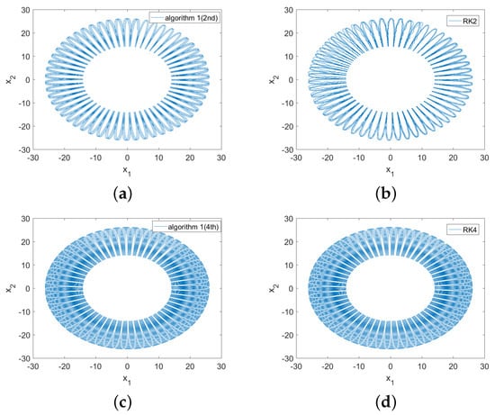
Figure 1. The phase orbit and the energy evolution obtained by Algorithm 1 and the Runge–Kutta methods. Subfigure (a) is the phase orbit obtained by the Algorithm 1 applied to the EP2 method with $\lambda =0.6$. Subfigure (b) is the orbit obtained by the RK2 method. In both subfigures (a,b), the stepsize is $h=\frac{\pi }{2}$ and the time interval is $[0,{10}^5\pi ]$. Subfigure (c) is the orbit obtained by the Algorithm 1 applied to the EP4 method with $\lambda =0.6$. Subfigure (d) is the orbit obtained by the RK4 method. In both subfigures (c,d), the stepsize is $h=\frac{\pi }{2}$ and the time interval is $[0,2\times {10}^5\pi ]$.

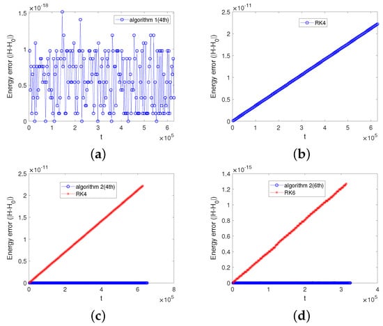
Figure 2. The energy evolution obtained by the two algorithms and the Runge–Kutta methods. Displayed in subfigure (a) is the energy error of Algorithm 1(4th) with $\lambda =0.5$. Subfigure (b) is the energy error of the RK4 method. In both subfigures (a,b), the time stepsize is $h=\frac{\pi }{2}$ and the time interval $[0,2\times {10}^5\pi ]$. Subfigure (c) is the comparison of the energy error between the Algorithm 2(4th) ($\lambda =0.3$) and the RK4 method with the time stepsize being $h=\frac{\pi }{2}$ and the time interval being $[0,2\times {10}^5\pi ]$. Subfigure (d) is the comparison of the energy error between the Algorithm 2(6th) ($\lambda =0.6$) and the RK6 method, with the time stepsize being $h=\frac{\pi }{2}$ and the time interval being $[0,{10}^5\pi ]$.

We compare the energy errors of the two adaptive algorithms with the energy-preserving methods without adaptive strategies (the EP4 method and the EP6 method), and the numerical results are displayed in Figure 3. The energy errors of the EP4 method and the EP6 method increase with time and show energy drift. But the energy errors of Algorithms 1 and 2 can be bounded over a long time and do not show energy drift. As can be seen from Figure 3, the energy error of Algorithm 2(4th) is three orders of magnitude smaller than that of the EP4 method and the energy error of the Algorithm 1(6th) is three orders of magnitude smaller than that of the EP6 method. This clearly shows the advantage of the two adaptive energy-preserving methods in long-term energy conservation over the energy-preserving methods without using adaptive strategies. Table 1 shows the global error of variable $\mathbf{X}$ of the first adaptive algorithm (Algorithm 1) over the time interval $[0,\mathrm{10,000}\pi ]$. As can be seen from Table 1, at the stepsize $\pi /8$, the error of Algorithm 1 applied to the EP2 method is about three orders of magnitude larger than that of Algorithm 1 applied to the EP4 method. At stepsize $\pi /2$, the error of Algorithm 1 applied to the EP4 method is about two orders of magnitude larger than that of Algorithm 1 applied to the EP6 method. The error of the sixth-order adaptive algorithm is small and achieves an order of magnitude of ${10}^{-8}$. This shows the necessity of constructing the higher-order energy-preserving method.

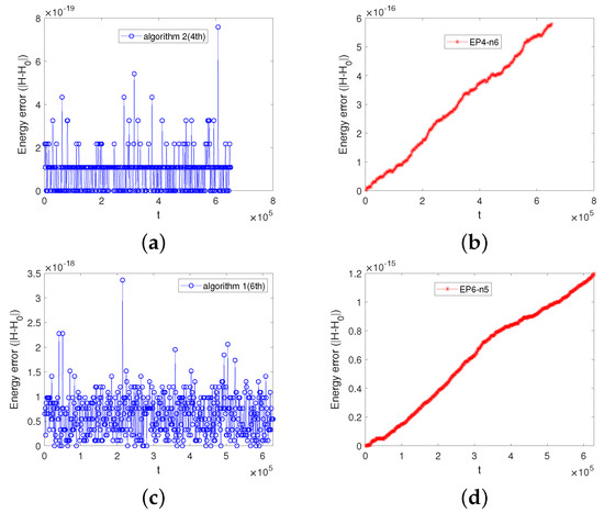
Figure 3. The energy evolution obtained by the two algorithms and the energy-preserving methods EP4 and EP6. Subfigure (a) is the result for the Algorithm 2(4th) ($\lambda =0.6$), subfigure (b) is the result for the EP4 method using the six-point Gauss–Legendre quadrature rule. In subfigures (a,b), the stepsize is $h=\frac{\pi }{2}$, and the total steps is $N=4\times {10}^5$. Subfigure (c) shows the results for Algorithm 1(6th) ($\lambda =0.2$), subfigure (d) shows the results for the EP6 method using the five-point Gauss–Legendre’s quadrature rule. In subfigures (c,d), the stepsize is $h=\frac{\pi }{2}$ and the total number of steps is $N=4\times {10}^5$.

Table 1. The global error of variable $\mathbf{X}$ in Example 1. The time interval is $[0,\mathrm{10,000}\pi ]$. The “***” means that we don’t calculate the values.

h	Algorithm 1(2nd)	Order	Algorithm 1(4th)	Order	Algorithm 1(6th)	Order
2$\pi$	***	***	$1.00749\times {10}^{-3}$	***	$1.41925\times {10}^{-4}$	***
$\pi$	$3.37452\times {10}^{-3}$	***	$6.67869\times {10}^{-5}$	3.91507	$2.60793\times {10}^{-6}$	5.76608
$\pi$/2	$9.83293\times {10}^{-4}$	1.77899	$4.24294\times {10}^{-6}$	3.97643	$6.14455\times {10}^{-8}$	5.40745
$\pi /4$	$2.46957\times {10}^{-4}$	1.99336	$2.76951\times {10}^{-7}$	3.93736	***	***
$\pi /8$	$6.16717\times {10}^{-5}$	2.00158	$4.53288\times {10}^{-8}$	2.61113	***	***

5.2.2. Example 2

We normalize the system according to natural units. The mass is set to be $m=1$ and the charge is set to be $q=1$. In this example, the magnetic field $B\left(\mathbf{X}\right)$ is

$$B\left(\mathbf{X}\right)=\left(0,\frac{x_1^2+x_3^2}{2},\sqrt{x_1^2+x_2^2}\right).$$

The scalar potential is $\phi \left(\mathbf{X}\right)=\frac{{10}^{-2}}{\sqrt{x_1^2+x_2^2}}$; therefore, we derive that the electric field

$$E\left(\mathbf{X}\right)=\frac{{10}^{-2}}{{(x_1^2+x_2^2)}^{3/2}}(x_1,x_2,0).$$

The Hamiltonian function is $H=\frac{1}{2}{v}_1^2+\frac{1}{2}{v}_2^2+\frac{1}{2}{v}_3^2+\phi \left(\mathbf{X}\right)$.

The initial condition is ${\mathbf{X}}_0=(0;-1;0)$ and ${\mathbf{V}}_0=(0.2;0.1;0)$. Displayed in Figure 4 are the energy errors obtained by Algorithms 1 and 2, the RK4 method, and the RK6 method. The energy errors of the two adaptive energy-preserving methods can be bounded by the machine precision over long time. The energy errors of the two Runge–Kutta methods increase without bounds. We can also see from Figure 4 that the energy error of Algorithm 1(4th) is ten orders of magnitude smaller than that of the RK4 method, while the energy error of Algorithm 2(6th) is nine orders of magnitude smaller than that of the RK6 method. When we compare the sixth-order adaptive energy-preserving method with the sixth-order Runge–Kutta method, we use a larger stepsize and we can see that the energy of the Algorithm 2(6th) can also be preserved over long time, but that of the RK6 method increases linearly with time. Figure 5 shows the comparison results in the energy error among Algorithms 1 and 2 and the same energy-preserving methods without using any adaptive strategy. We can see from Figure 5 that the energy error of Algorithm 1(4th) or Algorithm 1(6th) is smaller than the energy errors of the EP4 method or the EP6 method using three different points of Gauss–Legendre’s quadrature rules, respectively. Meanwhile, the energy error of Algorithm 2(4th) or Algorithm 2(6th) is smaller than the EP4 method or the EP6 method under the fixed time stepsize.

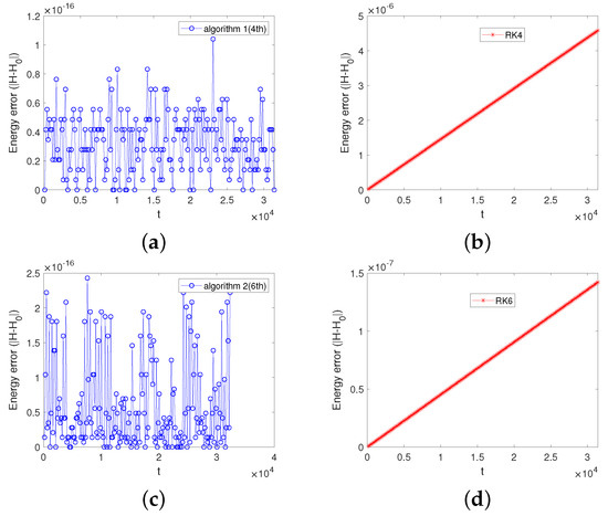
Figure 4. The energy errors obtained by the two algorithms and the Runge–Kutta methods. Subfigure (a) displays the energy error obtained by using Algorithm 1(4th) with $\lambda =0.1$. Subfigure (b) displays th energy error obtained by the RK4 method. In subfigures (a,b), the time stepsize is $h=\frac{\pi }{50}$ and the time interval is $[0,{10}^4\pi ]$. Subfigure (c) displays the energy error obtained by using Algorithm 2(6th) with $\lambda =0.7$. Subfigure (d) displays the energy error obtained by the RK6 method. In subfigures (c,d), the time stepsize is $h=\frac{\pi }{20}$ and the time interval is $[0,{10}^4\pi ]$.

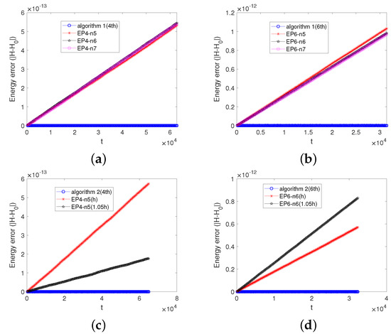
Figure 5. The energy evolution obtained by the two algorithms and the Runge–Kutta methods. Subfigure (a) displays the comparison among the energy errors obtained by using Algorithm 1(4th) and the EP4-n5, EP4-n6, and EP4-n7 methods. Subfigure (b) displays the comparison among the energy errors obtained by using Algorithm 1(6th) and the EP6-n5, EP6-n6, and EP6-n7 methods. Subfigure (c) displays Algorithm 2(4th) and the EP4 method under the stepsizes h and $1.05h$. Subfigure (d) displays Algorithm 2(6th) and the EP6 method under the stepsizes h and $1.05h$. In subfigures (a,c), the stepsize is $h=\frac{\pi }{50}$ and the time interval is $[0,2\times {10}^4\pi ]$, and in subfigures (b,d), $h=\frac{\pi }{20}$ and the time interval is $[0,{10}^4\pi ]$.

Table 2 shows the global error in variable $\mathbf{V}$ of Algorithm 1 applied to the EP2, EP4, and EP6 methods over the time interval $[0,1000\pi ]$. As can be seen from the table, under the stepsize $\pi /320$, the error of Algorithm 1(4th) is about four orders of magnitudes smaller than that of Algorithm 1(2nd). And under the stepsize $\pi /80$, the error of Algorithm 1(6th) is about three orders of magnitudes smaller than that of Algorithm 1(4th). Even under a very small stepsize of $\pi /320$, the error in $\mathbf{V}$ of Algorithm 1(2nd) is at the order of magnitude ${10}^{-3}$, and the error is a bit large. But the sixth-order method can achieve the error at the order of magnitude ${10}^{-4}$ under a big time stepsize $\pi /20$. This demonstrates that it is of importance to construct higher-order energy-preserving methods to acquire higher accuracy.

Table 2. The global error of variable $\mathbf{V}$ in Example 2. The time interval is $[0,1000\pi ]$. The “***” means that we don’t calculate the values.

h	Algorithm 1(2nd)	Order	Algorithm 1(4th)	Order	Algorithm 1(6th)	Order
$\pi /10$	***	***	$1.82879\times {10}^{-1}$	***	$1.57842\times {10}^{-2}$	***
$\pi /20$	***	***	$1.20875\times {10}^{-2}$	3.91930	$2.72253\times {10}^{-4}$	5.85739
$\pi /40$	$2.96856\times {10}^{-1}$	***	$7.61940\times {10}^{-4}$	3.98769	$4.33842\times {10}^{-6}$	5.97163
$\pi /80$	$8.04522\times {10}^{-2}$	1.88356	$4.76892\times {10}^{-5}$	3.99794	$3.69632\times {10}^{-8}$	6.87494
$\pi /160$	$2.01712\times {10}^{-2}$	1.99583	$2.94191\times {10}^{-6}$	4.01884	***	***
$\pi /320$	$5.04104\times {10}^{-3}$	2.00050	$1.41323\times {10}^{-7}$	4.37968	***	***

5.3. Numerical Results in Guiding Center System

We set the vector potential as

$$\mathbf{A}=\frac{B_0{r}^2}{2\sqrt{x^2+y^2}q}{e}_{\zeta }-ln\left(\frac{\sqrt{x^2+y^2}}{R_0}\right)\frac{R_0{B}_0}{2}{e}_z+\frac{B_0{R}_{0}z}{2\sqrt{x^2+y^2}}{e}_R,$$

(50)

where q, $B_0$, and $R_0$ are constants. The toroidal coordinates are $\eta =arctan\left(\frac{x}{y}\right)$ and $R=\sqrt{x^2+y^2}$. As a result, we can derive the magnetic field $\mathbf{B}\left(\mathbf{X}\right)$, the strength of the magnetic field $B\left(\mathbf{X}\right)$, and the unit vector along the magnetic field $\mathbf{b}\left(\mathbf{X}\right)$ as follows:

$$\begin{array}{cc}\hfill \mathbf{B}\left(\mathbf{x}\right)& =\frac{B_{0}r}{q\sqrt{x^2+y^2}}{e}_{\theta }+\frac{B_0{R}_0}{\sqrt{x^2+y^2}}{e}_{\zeta }=\frac{B_0{r}^2}{q\sqrt{x^2+y^2}}\nabla \theta -B_0{R}_0\nabla \zeta ,\hfill \\ \hfill B\left(\mathbf{x}\right)& =\frac{B_0}{q\sqrt{x^2+y^2}}\sqrt{r^2+R_0^2{q}^2},\hfill \\ \hfill \mathbf{b}\left(\mathbf{x}\right)& =(\frac{-xz-R_{0}qy}{\sqrt{x^2+y^2}\sqrt{r^2+R_0^2{q}^2}},\frac{-yz+R_{0}qx}{\sqrt{x^2+y^2}\sqrt{r^2+R_0^2{q}^2}},\frac{\sqrt{x^2+y^2}-R_0}{\sqrt{r^2+R_0^2{q}^2}}).\hfill \end{array}$$

(51)

where $\theta =arctan\left(\frac{z}{\sqrt{x^2+y^2}-R_0}\right)$ and $r=\sqrt{(\sqrt{x^2+y^2}-R_0)+z^2}$ are the poloidal coordinates.

Here, we report the numerical experiments for two different orbits of the guiding center system.

5.3.1. Banana Orbit

For the banana orbit, the initial value $Z_0$ is chosen to be $[1.05;0;0;0.0004306]$ and the magnetic moment $\mu$ is $2.25\times {10}^{-6}$. Displayed in Figure 6 are the banana orbits projected on the $(R,z)$ plane obtained by Algorithm 1(2nd), Algorithm 1(4th), the RK2 method, and the RK4 method. Figure 6 shows that the shape of the banana orbit can be nearly preserved by the Algorithm 1(2nd). But the banana orbit obtained by the RK2 method spirals outwards and loses accuracy. This clearly shows the advantage of the second-order adaptive energy-preserving algorithm in orbit preservation over the second-order Runge–Kutta method. As is also shown in Figure 6, the phase orbit of Algorithm 1(4th) and that of the RK method are not much different. Figure 7 displays the energy evolutions of Algorithm 1(4th), Algorithm 2(6th), the RK4 method, and the RK6 method. As can be seen from Figure 6, the energy error of Algorithm 1(4th) is eight orders of magnitude smaller than that of the RK4 method. Meanwhile, the energy error of Algorithm 2(6th) is five orders of magnitude smaller than that of the RK6 method. The energy errors of the two adaptive energy-preserving methods can be bounded at the order of magnitude ${10}^{-15}$ over the long term. But the energy errors of both the RK4 and the RK6 methods increase with time and do not show any boundedness. This demonstrates the significant advantage of the two adaptive energy-preserving algorithms in long-term energy conservation over the two Runge–Kutta methods.

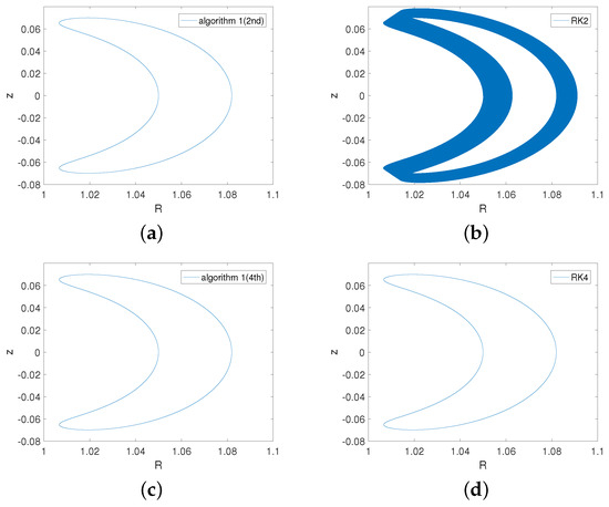
Figure 6. The banana orbit obtained by using Algorithm 1 applied to the EP4 and EP6 methods with $\lambda =0.5$ and the Runge–Kutta methods. Subfigure (a) is the banana orbit obtained by the Algorithm 1 applied to the EP2 method. Subfigure (b) is the orbit obtained by the RK2 method. Subfigure (c) is the orbit obtained by the Algorithm 1 applied to the EP4 method. Subfigure (d) is the orbit obtained by the RK4 method. The time stepsize $h=100$ and the time interval is $[0,5\times {10}^6]$.

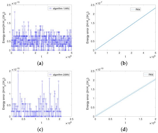
Figure 7. The energy errors obtained by the two algorithms and the Runge–Kutta methods. Subfigure (a) displays the energy evolution obtained by using Algorithm 1(4th) with $\lambda =0.8$. Subfigure (b) displays the energy evolution obtained by the RK4 method. In subfigures (a,b), the time stepsize is $h=100$ and the time interval is $[0,5\times {10}^6]$. Subfigure (c) displays the energy evolution obtained by using Algorithm 2(6th) with $\lambda =0.1$. Subfigure (d) displays the energy evolution obtained by the RK6 method. In subfigures (c,d), the time stepsize is $h=200$ and the time interval is $[0,2\times {10}^6]$.

We compare the energy errors of the two adaptive algorithms with the energy-preserving methods without adaptive strategies (the EP4 method and the EP6 method), and the numerical results are displayed in Figure 8. Both the EP4 and the EP6 methods show energy drift over the long term. The energy drift problem cannot be eliminated by the method using more points of Gauss-Legendre’s quadrature rule or using different fixed time stepsizes. But by using two adaptive strategies, we can see from Figure 8 that the two adaptive algorithms can preserve the energy error over long time and do not show any energy drift. This clearly shows that the energy drift problem is eliminated by using adaptive strategies. Table 3 shows the global error of variable $\mathbf{X}$ of the first adaptive algorithm (Algorithm 1) over the time interval $[0,{10}^5]$. As can be seen from Table 3, at the stepsize $100/2$, the error of Algorithm 1 applied to the EP2 method is about three orders of magnitude larger than that of Algorithm 1 applied to the EP4 method. Meanwhile, the error of Algorithm 1 applied to the EP4 method is about two orders of magnitude larger than that of Algorithm 1 applied to the EP6 method. It is important to construct higher-order energy-preserving methods.

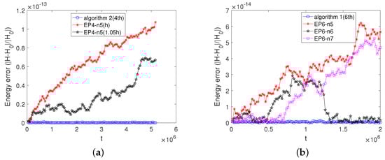
Figure 8. The energy evolution obtained by the two algorithms and the EP4 and EP6 methods. Subfigure (a) displays Algorithm 2(4th) with $\lambda =0.3$ and the EP4-n5 method under the stepsize h and $1.05h$. Subfigure (b) displays Algorithm 1(6th) with $\lambda =0.4$ and the EP6-n5, EP6-n6, and EP6-n7 methods. The time stepsize is $h=100$.

Table 3. The global error of variable $\mathbf{X}$ for the banana orbit. The time interval is $[0,{10}^5]$. The “***” means that we don’t calculate the values.

h	Algorithm 1(2nd)	Order	Algorithm 1(4th)	Order	Algorithm 1(6th)	Order
400	$1.54750\times {10}^{-1}$	***	$1.65831\times {10}^{-2}$	***	$4.74577\times {10}^{-3}$	***
200	$3.87522\times {10}^{-2}$	1.99759	$1.14773\times {10}^{-3}$	3.85286	$7.28696\times {10}^{-5}$	6.02518
100	$9.69199\times {10}^{-3}$	1.99941	$7.34576\times {10}^{-5}$	3.96573	$1.13343\times {10}^{-6}$	6.00655
100/2	$2.42326\times {10}^{-3}$	1.99984	$4.61575\times {10}^{-6}$	3.99227	$1.53947\times {10}^{-8}$	6.20212
100/4	$6.05824\times {10}^{-4}$	1.99998	$2.86555\times {10}^{-7}$	4.00968	***	***

5.3.2. Transit Orbit

For the transit orbit, the initial value $Z_0$ is chosen to be $[1.05;0;0;0.000804]$ and the magnetic moment $\mu$ is $2.448\times {10}^{-6}$. Figure 9 shows the advantage of Algorithm 1(2nd) in tracing the transit orbit over the RK2 method. Figure 10 demonstrates the superior advantage of the two adaptive energy-preserving algorithms in long-term energy conservation over the two Runge–Kutta methods. The relative energy errors of the two adaptive energy-preserving algorithms approximates the accuracy of the machine precision, but the relative energy errors of the two Runge–Kutta methods increase with time. Figure 11 shows that the two adaptive energy-preserving algorithms do not show energy drift over long time. But the energy-preserving methods not using the adaptive strategy clearly show the energy drift even we use more points of the Gaussian qudrature or choose a different stepsize in one method. Table 4 shows the global error in variable u of Algorithm 1 applied to the EP2, EP4, and EP6 method over the time interval $[0,{10}^5]$. At a stepsize of $100/16$, the error of Algorithm 1(4th) is about four orders of magnitude smaller than that of Algorithm 1(2nd). At a stepsize of $100/2$, the error of Algorithm 1(6th) is about three orders of magnitude smaller than that of Algorithm 1(4th). As can also be seen from Table 4, the higher-order methods can achieve smaller errors at big time stepsizes.

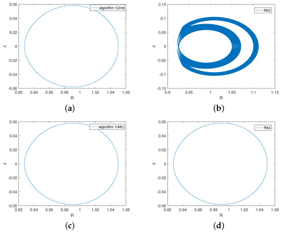
Figure 9. The transit orbit obtained by using Algorithm 1 applied to the EP4 and EP6 methods with $\lambda =0.4$ and the Runge–Kutta methods. Subfigure (a) is the transit orbit obtained by the Algorithm 1 applied to the EP2 method. Subfigure (b) is the orbit obtained by the RK2 method. Subfigure (c) is the orbit obtained by the Algorithm 1 applied to the EP4 method. Subfigure (d) is the orbit obtained by the RK4 method. The time stepsize is $h=100$ and the time interval is $[0,2\times {10}^6]$.

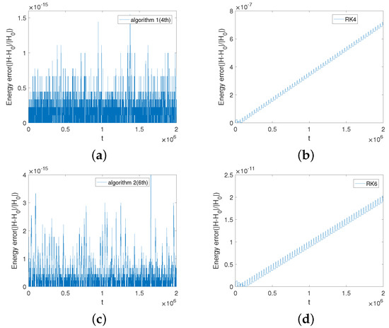
Figure 10. The energy errors obtained by the two algorithms and the Runge–Kutta methods. Subfigure (a) displays the energy evolution obtained by using Algorithm 1(4th) with $\lambda =0.5$. Subfigure (b) displays the energy evolution obtained by the RK4 method. In subfigures (a,b), the time stepsize is $h=100$ and the time interval is $[0,2\times {10}^6]$. Subfigure (c) displays the energy evolution obtained by using Algorithm 2(6th) with $\lambda =0.1$. Subfigure (d) displays th energy evolution obtained by the RK6 method. In subfigures (c,d), the time stepsize is $h=100$ and the time interval is $[0,2\times {10}^6]$.

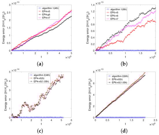
Figure 11. The energy evolution obtained by the two algorithms and the EP4, EP6 methods. Subfigure (a) displays the comparison results between Algorithm 1(4th) and the EP4-n5, EP4-n6, and EP4-n7 methods. Subfigure (b) displays the comparison results between Algorithm 1(6th) and the EP6-n5, EP6-n6, and EP6-n7 methods. Displayed in subfigure (c) are the results obtained by Algorithm 2(4th) and the EP4-n5 method under the stepsize h and $1.05h$. Displayed in subfigure (d) are the results obtained by Algorithm 2(6th) and the EP6-n5 method under the stepsize h and $1.05h$. The time stepsize is $h=100$.

Table 4. The global error of variable u for the transit orbit. The time interval is $[0,{10}^5]$. The “***” means that we don’t calculate the values.

h	Algorithm 1(2nd)	Order	Algorithm 1(4th)	Order	Algorithm 1(6th)	Order
400	***	***	$3.23592\times {10}^{-4}$	***	$6.24629\times {10}^{-5}$	***
200	***	***	$2.79239\times {10}^{-5}$	3.53460	$1.14288\times {10}^{-6}$	5.77225
100	***	***	$1.80063\times {10}^{-6}$	3.95493	$1.84300\times {10}^{-8}$	5.95447
100/2	$4.43129\times {10}^{-5}$	***	$1.13086\times {10}^{-7}$	3.99301	$2.90420\times {10}^{-10}$	5.98777
100/4	$1.13082\times {10}^{-5}$	1.97036	$7.07539\times {10}^{-9}$	3.99847	$4.78180\times {10}^{-12}$	5.92444
100/8	$2.84131\times {10}^{-6}$	1.99274	$4.42564\times {10}^{-10}$	3.99885	***	***
100/16	$7.11216\times {10}^{-7}$	1.99820	$2.79043\times {10}^{-11}$	3.98733	***	***

6. Conclusions

We have developed two adaptive higher-order symmetric energy-preserving algorithms for both the charged particle system and the guiding center system. The two adaptive algorithms adopt two adpative strategies: controlling the energy error by increasing the number of points of Gauss–Legendre’s quadrature rule or using two different stepsizes. The numerical results in the charged particle system and the guiding center system show that the two adaptive algorithms have superior advantages in long-term phase orbit preservation and energy preservation compared to the Runge–Kutta methods. Meanwhile, the numerical results also show that the two adaptive algorithms overcome the energy drift problem that occurs in the energy-preserving methods based on the averaged vector field. It is found that the two adaptive strategies used in the two adaptive energy-preserving methods can bound the energy error of higher-order methods to the machine’s precision.

References

- Feng, K. Collected Works of Feng Kang (II); National Defence Industry Press: Beijing, China, 1995; pp. 44–47. [Google Scholar]
- Hairer, E.; Lubich, C.; Wanner, G. Geometric Numerical Integration: Structure-Preserving Algorithms for Ordinary Differential Equations; Springer: Berlin/Heidelberg, Germany, 2002. [Google Scholar]
- Sanz-Serna, J.M.; Calvo, M.P. Numerical Hamiltonian Problems; Chapman and Hall: London, UK, 1994. [Google Scholar]
- Zajac, M.; Sardon, C.; Ragnisco, O. Time-dependent Hamiltonian mechanics on a locally conformal symplectic manifold. Symmetry 2023, 15, 843. [Google Scholar] [CrossRef]
- Yu, C.B.; Youn, J.R.; Song, Y.S. Encapsulated phase change material embedded by graphene powders for smart and flexible thermal response. Fibers Polym. 2019, 20, 545–554. [Google Scholar] [CrossRef]
- Yu, C.B.; Youn, J.R.; Song, Y.S. Tunable Electrical Resistivity of Carbon Nanotube Filled Phase Change Material Via Solid-solid Phase Transitions. Fibers Polym. 2020, 21, 24–32. [Google Scholar] [CrossRef]
- Feng, K. On Difference Schemes and Symplectic Geometry. In Proceedings of the 1984 Beijing Symposium on Differential Geometry and Differential Equations; Feng, K., Ed.; Science Press: Beijing, China, 1985; pp. 42–58. [Google Scholar]
- Feng, K.; Qin, M.Z. Symplectic Geometric Algorithms for Hamiltonian System; Springer: New York, NY, USA, 2009. [Google Scholar]
- Tang, Y.F.; Pérez-García, V.M.; Vázquez, L. Symplectic Methods for the Ablowitz-Ladik Model. Appl. Math. Comput. 1997, 82, 17–38. [Google Scholar] [CrossRef]
- Zhang, R.L.; Qin, H.; Tang, Y.F.; Liu, J.; He, Y.; Xiao, J.Y. Explicit symplectic algorithms based on generating functions for charged particle dynamics. Phys. Rev. E 2016, 94, 013205. [Google Scholar] [CrossRef] [PubMed]
- Zhang, R.L.; Wang, Y.L.; He, Y.; Xiao, J.Y.; Liu, J.; Qin, H.; Tang, Y.F. Explicit symplectic algorithms based on generating functions for relativistic charged particle dynamics in time-dependent electromagnetic field. Phys. Plasmas 2018, 25, 022117. [Google Scholar] [CrossRef]
- Bader, P.; Blanes, S.; Casas, F.; Kopylov, N. Symplectic propagators for the Kepler problem with time-dependent mass. Celest. Mech. Dyn. Astron. 2019, 131, 25. [Google Scholar] [CrossRef]
- Elenin, G.G.; Elenin, T.G. Adaptive symplectic conservative numerical methods for the Kepler problem. Diff. Equat. 2017, 53, 923–934. [Google Scholar] [CrossRef]
- Chen, Y.L.; Wu, X. Application of force gradient symplectic integrators to the circular restricted three-body problem. Acta Phys. Sin. 2013, 62, 140501. [Google Scholar] [CrossRef]
- Zhang, Y.Y.; Li, Y.J.; Li, N. Numerical algorithms for solving restricted three body problem. Appl. Mech. Mater. 2011, 40, 917–923. [Google Scholar] [CrossRef]
- Blanes, S.; Moan, C.P. Splitting methods for non-autonomous Hamiltonian equations. J. Comput. Phys. 2001, 170, 205–230. [Google Scholar] [CrossRef]
- Zhu, B.B.; Tang, Y.F.; Liu, J. Energy-preserving methods for guiding center system based on averaged vector field. Phys. Plasmas 2022, 29, 032501. [Google Scholar] [CrossRef]
- Zhu, B.B.; Liu, J.; Zhang, J.W.; Zhu, A.Q.; Tang, Y.F. Adaptive energy-preserving algorithms for guiding center system. Plasma Sci. Technol. 2023, 25, 045102. [Google Scholar] [CrossRef]
- Albosaily, S.; Mohammed, W.W.; Aiyashi, M.A.; Abdelrahman, M.A.E. Exact solutions of the (2+1)-dimensional stochastic chiral nonlinear Schrödinger equation. Symmetry 2020, 12, 1874. [Google Scholar] [CrossRef]
- Shah, N.A.; Agarwal, P.; Chung, J.D.; El-Zahar, E.R.; Hamed, Y.S. Analysis of optical solitons for nonlinear Schrödinger equation with detuning term by iterative transform method. Symmetry 2020, 12, 1850. [Google Scholar] [CrossRef]
- Qin, H.; Guan, X. Variational Symplectic Integrator for Long-Time Simulations of the Guiding-Center Motion of Charged Particles in General Magnetic Fields. Phys. Rev. Lett. 2008, 100, 035006. [Google Scholar] [CrossRef] [PubMed]
- He, Y.; Zhou, Z.Q.; Sun, Y.J.; Liu, J.; Qin, H. Explicit K-symplectic algorithms for charged particle dynamics. Phys. Lett. A 2017, 381, 568–573. [Google Scholar] [CrossRef]
- Lu, Y.L.; Yuan, J.B.; Tian, H.Y.; Qin, Z.W.; Chen, S.Y.; Zhou, H.J. Explicit K-symplectic and symplectic-like methods for charged particle system in general magnetic field. Symmetry 2023, 15, 1146. [Google Scholar] [CrossRef]
- Zhu, B.B.; Tang, Y.F.; Zhang, R.L.; Zhang, Y.H. Symplectic simulation of dark solitons motion for nonlinear Schrödinger equation. Numer. Algorithms 2019, 81, 1485–1503. [Google Scholar] [CrossRef]
- Zhu, B.B.; Zhang, R.L.; Tang, Y.F.; Tu, X.B.; Zhao, Y. Splitting K-symplectic methods for non-canonical separable Hamiltonian problems. J. Comput. Phys. 2016, 322, 387–399. [Google Scholar] [CrossRef]
- Brugnano, L.; Zhang, C.J.; Li, D.F. A class of energy-conserving Hamiltonian boundary value methods for nonlinear Schrödinger equation with wave operator. Commun. Nonlin. Sci. Numer. Simulat. 2018, 60, 33–49. [Google Scholar] [CrossRef]
- Brugnano, L.; Iavernaro, F. Line Integral Methods for Conservative Problems; Chapman and Hall/CRC: Boca Raton, FL, USA, 2016. [Google Scholar]
- Wu, X.Y.; Wang, B.; Shi, W. Efficient energy-preserving integrators for oscillatory Hamiltonian systems. J. Comput. Phys. 2013, 235, 587–605. [Google Scholar] [CrossRef]
- He, Y.; Sun, Y.J.; Zhang, R.L.; Wang, Y.L.; Liu, J.; Qin, H. High order volume-preserving algorithms for relativistic charged particles in general electromagnetic fields. Phys. Plasmas 2016, 23, 092109. [Google Scholar] [CrossRef]
- Shang, Z.J. Construction of volume-preserving difference schemes for source-free systems via generating functions. J. Comput. Math. 1994, 12, 265–272. [Google Scholar]
- Shang, Z.J. Generating functions for volume-preserving mappings and Hamilton-Jacobi equations for source-free dynamical systems. Sci. China Ser. A 1994, 37, 1172–1188. [Google Scholar]
- Quispel, G.R.W.; Turner, G.S. Discrete gradient methods for solving ODEs numerically while preserving a first integral. J. Phys. A Math. Gen. 1996, 29, L341–L349. [Google Scholar] [CrossRef]
- Celledoni, E.; Grimm, V.; McLachlan, R.I.; McLaren, D.I.; O’Neale, D.; Owren, B.; Quispel, G.R.W. Preserving energy resp. dissipation in numerical PDEs using the “Average Vector Field” method. J. Comput. Phys. 2012, 231, 6770. [Google Scholar] [CrossRef]
- Li, H.C.; Wang, Y.S. An averaged vector field Legendre spectral element method for the nonlinear Schrödinger equation. Int. J. Comput. Math. 2016, 94, 1196–1218. [Google Scholar] [CrossRef]
- Brugnano, L.; Montijano, J.I.; Randez, L. High-order energy-conserving line integral methods for charged particle dynamics. J. Comput. Phys. 2019, 396, 209–227. [Google Scholar] [CrossRef]
- Li, H.C.; Wang, Y.S. A discrete line integral method of order two for Lorentz force system. Appl. Math. Comput. 2016, 291, 207–212. [Google Scholar] [CrossRef]
- Tang, R.; Li, D. On Symmetric Methods for Charged Particle Dynamics. Symmetry 2021, 13, 1626. [Google Scholar] [CrossRef]
- Li, T.; Wang, B. Efficient energy-preserving methods for charged-particle dynamics. Appl. Math. Comput. 2019, 361, 703–714. [Google Scholar] [CrossRef]
- Li, T.; Wang, B. Arbitrary-order energy-preserving methods for charged-particle dynamics. Appl. Math. Lett. 2020, 100, 106050. [Google Scholar] [CrossRef]
- Zhang, R.L.; Liu, J.; Hong, Q.; Tang, Y.F. Energy-preserving algorithm for gyrocenter dynamics of charged particles. Numer. Algorithms 2019, 81, 1521–1530. [Google Scholar] [CrossRef]
- Gonzalez, O. Time integration and discrete Hamiltonian systems. J. Nonlinear Sci. 1996, 6, 449–467. [Google Scholar] [CrossRef]
- Littlejohn, R. A guiding center Hamiltonian: A new approac. J. Math. Phys. 1979, 20, 2445–2458. [Google Scholar] [CrossRef]
- Yoshida, H. Construction of higher order symplectic integrators. Phys. Lett. A 1990, 150, 262. [Google Scholar] [CrossRef]
- Hairer, E.; Nørsett, S.P.; Wanner, G. Solving Ordinary Differential Equation I: Nonstiff Problems; Springer: Berlin/Heidelberg, Germany, 1987. [Google Scholar]
- Butcher, J.C. Implicit Runge-Kutta Processes. Math. Comput. 1964, 18, 50–64. [Google Scholar] [CrossRef]
Disclaimer/Publisher’s Note: The statements, opinions and data contained in all publications are solely those of the individual author(s) and contributor(s) and not of MDPI and/or the editor(s). MDPI and/or the editor(s) disclaim responsibility for any injury to people or property resulting from any ideas, methods, instructions or products referred to in the content. |
© 2023 by the authors. Licensee MDPI, Basel, Switzerland. This article is an open access article distributed under the terms and conditions of the Creative Commons Attribution (CC BY) license (https://creativecommons.org/licenses/by/4.0/).