Article

On Non-Symmetric Fractal-Fractional Modeling for Ice Smoking: Mathematical Analysis of Solutions

1
Department of Mathematics, University of Malakand, Dir Lower, Chakdara 18800, Khyber Pakhtunkhwa, Pakistan
2
Department of Mathematics and Sciences, Prince Sultan University, Riyadh 11586, Saudi Arabia
3
Department of Mathematics, Shaheed Benazir Bhutto University, Dir Upper, Sheringal 18050, Khyber Pakhtunkhwa, Pakistan
4
Department of Electricity and Electronics, Institute of Research and Development of Processes, Faculty of Science and Technology, University of the Basque Country (UPV/EHU), 48940 Leioa, Bizkaia, Spain
5
Department of Industrial Engineering, OSTİM Technical University, Ankara 06374, Türkiye
6
Department of Mathematics, Azarbaijan Shahid Madani University, Tabriz 3751-71379, Iran
7
Department of Mathematics, College of Natural Sciences, Jimma University, Jimma P.O. Box 378, Ethiopia
8
Department of Medical Research, China Medical University Hospital, China Medical University, Taichung 40402, Taiwan
*
Authors to whom correspondence should be addressed.
Symmetry 2023, 15(1), 87; https://doi.org/10.3390/sym15010087
Submission received: 6 December 2022 / Revised: 19 December 2022 / Accepted: 26 December 2022 / Published: 29 December 2022
(This article belongs to the Section Mathematics)

Abstract

:
Drugs have always been one of the most important concerns of families and government officials at all times, and they have caused irreparable damage to the health of young people. Given the importance of this great challenge, this article discusses a non-symmetric fractal-fractional order ice-smoking mathematical model for the existence results, numerical results, and stability analysis. For the existence of the solution of the given ice-smoking model, successive iterative sequences are defined. The uniqueness of the solution Hyers–Ulam (HU) stability is established with the help of the existing definitions and theorems in functional analysis. By the utilization of two-step Lagrange polynomials, we provide numerical solutions and provide a comparative numerical analysis for different values of the fractional order and fractal order. The numerical simulations show the applicability of the scheme and future prediction and the effects of fractal-fractional orders simultaneously.

1. Introduction

Arab traders discovered and recognized the poppy plant (Opium) for the first time in Southwestern China and India in the 7th century. It was used as a medicine for various diseases. The cultivation of this plant was rare, but it became prevalent in the 15th century when European traders boosted their trades to these regions, see [1]. The European merchants were exchanging gold and silver with the Chinese and easterners for spices and silk. In [2], Cady says that in the 17th century, the Chinese people started smoking a mixture of tobacco and opium. This provided an opportunity for the Europeans to become rich and recoup their money from the Chinese by supplying opium from colonial India in the late 18th century. According to [1], the British started to supply 15 million opium addicts in China. The cultivation of the poppy crop spread in India and even to Myanmar and Laos, bringing profit to the Europeans. Millions of Asians became addicted to opium, and up to 1970s, all of the opium produced in this region was consumed by opium-addicted Asians.
In this era, the narcotics syndicate arrived, and they started the refinement of opium into heroin. The Sicilian Mafia introduced heroin into Europe and propagated it there. Legally produced opium from Turkey was taken to France and Marseille for refinement into heroin and transferred to the United States and Western Europe. It is a confirmed reality that drugs have ruined the lives of the millions people throughout the world. Germany, Japan, Pakistan, and the United States are the countries where the proportion of drug addicts is alarming. Morphine, churse, heroin, ice (methamphetamine), cannabis, and cocaine are the very common drugs. Among these drugs, ice claims the most addicts worldwide. According to a paper from Dr. Nowshad Khan and Shah Fahad [3], for the first time in world history, ice was used as drug in Japan in 1919; it was prepared in laboratories in 1960, although, as Philip Jenkins in [4] states, it did not become the main concern of the media and politicians until 1989 and 1990. Philip further explains that ice (smokable crystal methamphetamine) was a threat to American society. It was used by the army persons in World War II for prolonged duties. Ice stimulates one’s hormones and speeds up one’s activities by up to one thousand times. In the beginning, it provides extreme pleasure, but with the passage of time, it destroys cells in the body. Nowshad and Fahad state that doctors have reported that ice increases one’s heart rate and blood pressure, and it gradually makes humans lazy and weak.
To study the effects of such dangerous drugs in more detail, many different articles have been published in which researchers conduct various types of scientific research based on various mathematical data and models. Some of them can be mentioned, including [5,6,7]. In 2013, Zeb et al. [8] designed a square-root-structured model of giving up smoking and analyzed it via the finite difference method. In the same year, Huo et al. [9] investigated the effect of relapse on the cessation of smoking in the context of a mathematical model. Recently, in 2018, Zeb et al. published two papers on the dynamics of cigarette smoking [10,11]. Similar to them, one can mention the other works done by other researchers such as [12,13,14,15,16]. In the meantime, we can even see the high efficiency of mathematical models in studying the properties and dynamics of various processes and diseases, including the mathematical models of thermostat control [17], anthrax in animals [18], mosaic disease [19], Q fever [20], memristor-based circuits [21], Mump virus [22], the hybrid system of p-Laplacial operators [23], and other biologic and engineering models [24,25,26,27,28,29,30,31,32,33].
Our main purpose in this paper is the analysis of a mathematical system of the ice-smoking model with the help of the fractal-fractional operators. This specifies the motivation of our research; the application of the fractal-fractional operators for this model specifies the novelty of our research because we extend the previous results to a generalized system of fractal-fractional IVPs, and their simulations of the solutions of the mentioned system give more accurate results.
In this manuscript, the desired model of the fractal-fractional system is described in Section 2, and some preliminaries are stated in Section 3. Via the successive iterative sequences and limit points, we investigate the existence criterion in Section 4, and further, we verify its uniqueness in Section 5. By defining HU-stable solutions, we analyze this qualitative property for the given fractal-fractional ice-smoking model in Section 6. Furthermore, the two-step Lagrange polynomials help us to derive a numerical solution, and then we simulate the comparative results for different values of parameters of these fractal-fractional operators in Section 7. Lastly, we complete the research via the conclusion in Section 8.

2. Description of the Ice-Smoking Model

Recently, in 2021, Zeb and Alzahrani [34] studied the ice-smoking model based on the finite scheme along with the linear differential equation approach, which takes the form:
S ˙ ( t ) = λ β S C μ S , C ˙ ( t ) = β S C ( γ + μ + ρ 1 ) C + a C R , R ˙ ( t ) = γ C ( μ + ρ 2 ) R a C R , Q ˙ ( t ) = ρ 1 C + ρ 2 R μ Q .
We intend to discuss the same model by the non-symmetric fractal-fractional order structure with existence, uniqueness, stability, and numerical simulations. We proceed as follows:
0 F F M D t ν 1 , σ * S ( t ) = λ β S C μ S , 0 F F M D t ν , σ * C ( t ) = β S C ( γ + μ + ρ 1 ) C + a C R , 0 F F M D t ν 1 , σ * R ( t ) = γ C ( μ + ρ 2 ) R a C R , 0 F F M D t ν 1 , ρ * Q ( t ) = ρ 1 C + ρ 2 R μ Q ,
with initial conditions
S ( 0 ) = S 0 , C ( 0 ) = C 0 , R ( 0 ) = R 0 , Q ( 0 ) = Q 0 ,
with S 0 , C 0 , R 0 , Q 0 0 . Here, 0 F F M D t ν 1 , σ * stands for the fractal-fractional derivative in the Atangana–Baleanu sense for ν 1 , σ * ( 0 , 1 ] . In the model (1), the whole population is grouped into 4 classes. They are S ( t ) , which illustrates potential smokers and potential non-smokers. The mentioned compartment or class is increased under the rate λ , denoting the recruitment rate.
The compartment or category C(t) specifies the chain smokers. It is increased when potential smokers begin to smoke under an incidence rate or under the contact rate among the potential smokers β S ( t ) C ( t ) and a C ( t ) R ( t ) of the relapse smokers who have returned to smoking. Note that some other individuals will leave this category under the rates γ C ( t ) , ρ 1 C ( t ) and μ C ( t ) . Additionally, the category C ( t ) is increased under the rate γ C ( t ) in which γ is the rate at which regular smokers transfer to the reversion category. Moreover, C ( t ) is decreased under the rates μ R ( t ) , ρ 2 R ( t ) . Accordingly, Q ( t ) represents the permanent quitters.
In this model, λ is a parameter denoting the birth or migration rate to the host population. The rate μ shows the natural death in all four categories. The rate ρ 1 shows the number of regular smokers who quit, and the rate r h o 2 shows the number of reversion persons who quit. β is the incidence rate in relation to the susceptible persons to the class of the regular smokers. Additionally, a is the relapse rate, and the rate α shows the number of individuals who relapsed and became regular smokers.

3. Preliminaries

In this article, we presume the Banach’s space { ϕ ( t ) C ( [ 0 , 1 ] R ) } with the norm ϕ = max t [ 0 , 1 ] | ϕ ( t ) | . Here, we highlight the basic notions of the fractal-fractional calculus. This derivative is based on the Mittag–Leffler kernel, which is a non-singular kernel. This derivative is recently recommended by several authors for the dynamical problems and has many advantages too. Like other fractional derivatives, it possesses the potential to have the classical results as well new solutions for the fractal and fractional orders. Regarding the fractal-fractional operators and their basic notions, see [35,36].
Definition 1
([35,36]). Consider ϕ C ( ( a , b ) , R ) which is fractal differentiable on ( a , b ) of order 0 < ϱ * 1 . The fractal-fractional derivation operator for ϕ in the Atangana–Baleanu settings of order 0 < κ 1 1 , with the generalized kernel of the Mittag–Leffler type, is introduced as
0 F F M D t κ 1 , ϱ * ϕ ( t ) = A B ( κ 1 ) 1 κ 1 d d t ϱ * 0 t ϕ ( s ) E κ 1 κ 1 1 κ 1 ( t s ) κ 1 d s ,
where A B ( κ 1 ) = 1 κ 1 + κ 1 Γ κ 1 , and
d ϕ ( s ) d s ϱ * = lim t s ϕ ( t ) ϕ ( s ) t ϱ * s ϱ * .
Definition 2
([35,36]). Let ϕ be the same function considered above. Then, the fractal-fractional integration operator in the Atangana–Baleanu settings for ϕ of order 0 < κ 1 1 with the kernel of Mittag–Leffler type is given by
0 F F M I t κ 1 , ϱ * ϕ ( t ) = κ 1 ϱ * A B ( κ 1 ) Γ κ 1 0 t s ϱ * 1 ϕ ( s ) ( t s ) κ 1 1 d s + ϱ * ( 1 κ 1 ) t ϱ * 1 A B ( κ 1 ) ϕ ( t ) ,
where A B ( κ 1 ) = 1 κ 1 + κ 1 Γ κ 1 .
By making use of a successive iterative technique, we shall accomplish the proof for the existence criterion to the fractal-fractional model (1). For this, we operate the integral given in Definition 2 from [36] on the proposed model (1), and we have
S ( t ) S ( 0 ) = ν 1 σ * A B ( ν 1 ) Γ ν 1 0 t s σ * 1 ( t s ) ν 1 1 [ λ β S C μ S ] d s + σ * ( 1 ν 1 ) t σ * 1 A B ( ν 1 ) [ λ β S C μ S ] , C ( t ) C ( 0 ) = ν 1 σ * A B ( ν 1 ) Γ ν 1 0 t s σ * 1 ( t s ) ν 1 1 [ β S C ( γ + μ + ρ 1 ) C + a C R ] d s + σ * ( 1 ν 1 ) t σ * 1 A B ( ν 1 ) [ β S C ( γ + μ + ρ 1 ) C + a C R ] , R ( t ) R ( 0 ) = ν 1 σ * A B ( ν 1 ) Γ ν 1 0 t s σ * 1 ( t s ) ν 1 1 [ γ C ( μ + ρ 2 ) R a C R ] d s + σ * ( 1 ν 1 ) t σ * 1 A B ( ν 1 ) [ γ C ( μ + ρ 2 ) R a C R ] , Q ( t ) Q ( 0 ) = ν 1 σ * A B ( ν 1 ) Γ ν 1 0 t s σ * 1 ( t s ) ν 1 1 [ ρ 1 C + ρ 2 R μ Q ] d s + σ * ( 1 ν 1 ) t σ * 1 A B ( ν 1 ) [ ρ 1 C + ρ 2 R μ Q ] .
Regard the functions V i for i = 1 , 2 , , 4 or i N 1 4 , given below:
V 1 ( t , S ) = λ β S C μ S V 2 ( t , C ) = β S C ( γ + μ + ρ 1 ) C + a C R , V 3 ( t , R ) = γ C ( μ + ρ 2 ) R a C R , V 4 ( t , Q ) = ρ 1 C + ρ 2 R μ Q .

4. Existence Criteria

In the present part, for establishing the desired theorem on the existence property, we provide an assumption:
( H * ) All S ( t ) , S * ( t ) , C ( t ) , C * ( t ) , R ( t ) , R * ( t ) , Q ( t ) , Q * ( t ) L [ 0 , 1 ] are continuous so that S a 1 , C a 2 , R a 3 , Q a 4 for some positive constants a 1 , a 2 , a 3 , a 4 > 0 . Furthermore, we define the following constants: ϕ 1 = β a 2 + μ , ϕ 2 = β a 1 + ( γ + μ + ρ 1 ) + a a 3 , ϕ 3 = μ + ρ 2 + a a 2 , ϕ 4 = μ .
Theorem 1.
The Lipschitz condition is valid for the kernels V i for i N 1 4 if the assumption ( H * ) fulfills and ϕ i < 1 for i N 1 4 .
Proof. 
We first check V 1 ( t , S ) for the Lipschitz property. For this, we are helped by ( H * ) and (3) and obtain
V 1 ( S ) V 1 ( S * ) = ( λ β S C μ S ) ( λ β S * C μ S * ) ( β S S * C + μ S S * ( β a 2 + μ ) S S * = ϕ 1 S S * ,
where ϕ 1 = β a 2 + μ . Hence, V 1 satisfies the Lipchitz condition with the Lipchitz-constant ϕ 1 . Similarly, for V 2 ( t , C ) , we have
V 2 ( C ) V 2 ( C * ) = ( β S C ( γ + μ + ρ 1 ) C + a C R ) ( β S C * ( γ + μ + ρ 1 ) C * + a C * R ) β a 1 + ( γ + μ + ρ 1 ) + a a 3 C C * = ϕ 2 C C * ,
where ϕ 2 = β a 1 + ( γ + μ + ρ 1 ) + a a 3 . Hence, V 2 fulfills the Lipschitz property with constant ϕ 2 . For V 3 ( t , R ) , we also have
V 3 ( R ) V 3 ( R * ) = ( γ C ( μ + ρ 2 ) R a C R ) ( γ C ( μ + ρ 2 ) R * a C R * ) ( μ + ρ 2 ) ( R * R ) + a C ( R * R ) ( μ + ρ 2 + a C ) R R * = ( μ + ρ 2 + a a 2 ) R R * = ϕ 3 R R * ,
where ϕ 3 = μ + ρ 2 + a a 2 . This implies that V 3 satisfies the Lipchitz condition via constant ϕ 3 . Now, for V 4 ( t , Q ) , we have
V 4 ( Q ) V 4 ( Q * ) = ( ρ 1 C + ρ 2 R μ Q ) ( ρ 1 C + ρ 2 R μ Q * ) μ ( Q * Q ) = μ Q Q * = ϕ 4 Q Q * ,
where ϕ 4 = μ . Thus, V 4 also fulfills the Lipschitz property with constant ϕ 4 . Thus, from (4)–(7), we have that V i for i = 1 , 2 , , 4 , satisfy the Lipschitz property, and the result is accomplished. □
Let us assume:
S ( t ) S ( 0 ) = ν 1 σ * A B ( ν 1 ) Γ ν 1 0 t ( t s ) ν 1 1 s σ * 1 V 1 ( s , S ( s ) ) d s + σ * ( 1 ν 1 ) A B ( ν 1 ) t σ * 1 V 1 ( t , S ( t ) ) , C ( t ) C ( 0 ) = ν 1 σ * A B ( ν 1 ) Γ ν 1 0 t ( t s ) ν 1 1 s σ * 1 V 2 ( s , C ( s ) ) d s + σ * ( 1 ν 1 ) A B ( ν 1 ) t σ 0 * 1 V 2 ( t , C ( t ) ) , R ( t ) R ( 0 ) = ν 1 σ * A B ( ν 1 ) Γ ν 1 0 t ( t s ) ν 1 1 s σ * 1 V 3 ( s , R ( s ) ) d s + σ * ( 1 ν 1 ) A B ( ν 1 ) t σ * 1 V 3 ( t , R ( t ) ) , Q ( t ) R ( 0 ) = ν 1 σ * A B ( ν 1 ) Γ ν 1 0 t ( t s ) ν 1 1 s σ * 1 V 4 ( s , Q ( s ) ) d s + σ * ( 1 ν 1 ) A B ( ν 1 ) t σ * 1 V 4 ( t , Q ( t ) ) .
Now, we define the following recursive formulas for the model (1):
S n ( t ) S ( 0 ) = ν 1 σ * A B ( ν 1 ) Γ ν 1 0 t ( t s ) ν 1 1 s σ * 1 V 1 ( s , S n 1 ( s ) ) d s + σ * ( 1 ν 1 ) A B ( ν 1 ) t σ * 1 V 1 ( t , S n 1 ( t ) ) ,
C n ( t ) C ( 0 ) = ν 1 σ * A B ( ν 1 ) Γ ν 1 0 t ( t s ) ν 1 1 s σ * 1 V 2 ( s , C n 1 ( s ) ) d s + σ * ( 1 ν 1 ) A B ( ν 1 ) t σ * 1 V 2 ( t , C n 1 ( t ) ) ,
R n ( t ) R ( 0 ) = ν 1 σ * A B ( ν 1 ) Γ ν 1 0 t ( t s ) ν 1 1 s σ * 1 V 3 ( s , R n 1 ( s ) ) d s + σ * ( 1 ν 1 ) A B ( ν 1 ) t σ * 1 V 3 ( t , R n 1 ( t ) ) .
Q n ( t ) Q ( 0 ) = ν 1 σ * A B ( ν 1 ) Γ ν 1 0 t ( t s ) ν 1 1 s σ * 1 V 4 ( s , Q n 1 ) ( s ) ) d s + σ * ( 1 ν 1 ) A B ( ν 1 ) t σ * 1 V 4 ( t , Q n 1 ) ( t ) ) ,
Theorem 2.
Under assumption ( H * ) , the fractal-fractional ice-smoking model (1) has a solution if we have
Δ = max [ ϕ 1 , ϕ 2 , ϕ 3 , ϕ 4 ] < 1 .
Proof. 
We define four functions as follows:
U 1 n ( t ) = S n + 1 ( t ) S ( t ) , U 2 n ( t ) = C n + 1 ( t ) C ( t ) , U 3 n ( t ) = R n + 1 ( t ) R ( t ) , U 4 n ( t ) = Q n + 1 ( t ) Q ( t ) .
Then, we find that
U 1 n ( t ) = ν 1 σ * A B ( ν 1 ) Γ ν 1 0 t ( t s ) ν 1 1 s σ * 1 [ V 1 ( s , S n ( s ) ) V 1 ( s , S ( s ) ) ] d s + σ * ( 1 ν 1 ) A B ( ν 1 ) t σ * 1 [ V 1 ( t , S n ( t ) ) V 1 ( t , S ( t ) ) ] ν 1 σ * A B ( ν 1 ) Γ ν 1 0 t ( t s ) ν 1 1 s σ * 1 ϕ 1 S n S d s + σ * ( 1 σ 1 ) A B ( ν 1 ) t σ * 1 ϕ 1 S n S [ ν 1 σ * Γ ( σ * ) A B ( ν 1 ) Γ ( ν 1 + σ * ) + σ * ( 1 ν 1 ) A B ( ν 1 ) ] ϕ 1 S n S [ ν 1 σ * Γ ( σ * ) A B ( ν 1 ) Γ ( ν 1 + σ * ) + σ * ( 1 ν 1 ) A B ( ν 1 ) ] ϕ 1 S n S [ ν 1 Γ ( σ * + 1 ) A B ( ν 1 ) Γ ( ν 1 + σ * ) + σ * ( 1 ν 1 ) A B ( ν 1 ) ] n ϕ 1 n S 1 S .
In which, for ϕ 1 < 1 and as n , we have S n S . So, U 1 n 0 as n . Similarly,
U 2 n ( t ) [ ν 1 Γ ( σ * + 1 ) A B ( ν 1 ) Γ ( ν 1 + σ * ) + σ * ( 1 ν 1 ) A B ( ν 1 ) ] n ϕ 2 n C 1 C ,
U 3 n ( t ) [ ν 1 Γ ( σ * + 1 ) A B ( ν 1 ) Γ ( ν 1 + σ * ) + σ * ( 1 ν 1 ) A B ( ν 1 ) ] n ϕ 3 n R 1 R ,
U 4 n ( t ) [ ν 1 Γ ( σ * + 1 ) A B ( ν 1 ) Γ ( ν 1 + σ * ) + σ * ( 1 ν 1 ) A B ( ν 1 ) ] n ϕ 4 n Q 1 Q .
By (10)–(13), when n , then U i n ( t ) 0 , i N 2 4 , for ϕ i < 1 , ( i = 2 , , 4 ) . Ultimately, the ice-smoking system (1) has a solution. □

5. Unique Solution

For our suggested ice-smoking model (1), we follow the analysis of the uniqueness property.
Theorem 3.
The fractal-fractional ice-smoking model (1) possesses one solution exactly if ( H * ) is satisfied and the following holds:
ν 1 Γ ( σ * + 1 ) A B ( ν 1 ) Γ ( ν 1 + σ * ) + σ * ( 1 ν 1 ) A B ( ν 1 ) ϕ i 1 , i N 1 4 .
Proof. 
We assume that the conclusion of the theorem is not valid. In other words, another solution exists for the supposed ice-smoking (I M) model (1) in the fractal-fractional settings. Hence, S * ( t ) , C * ( t ) , R * ( t ) , Q * ( t ) is another solution with S * ( 0 ) = S 0 , C * ( 0 ) = C 0 , R * ( 0 ) = R 0 , Q * ( 0 ) = Q 0 s.t.
S * ( t ) S * ( 0 ) = ν 1 σ * A B ( ν 1 ) Γ ν 1 0 t ( t s ) ν 1 1 s σ * 1 V 1 ( s , S * ( s ) ) d s , + σ * ( 1 ν 1 ) A B ( ν 1 ) t σ * 1 V 1 ( t , S * ( t ) ) ,
and similarly,
C * ( t ) C * ( 0 ) = ν 1 σ * A B ( ν 1 ) Γ ν 1 0 t ( t s ) ν 1 1 s σ * 1 V 2 ( s , C * ( s ) ) d s + σ * ( 1 ν 1 ) A B ( ν 1 ) t σ * 1 V 2 ( t , C * ( t ) ) ,
R * ( t ) R * ( 0 ) = ν 1 σ * A B ( ν 1 ) Γ ν 1 0 t ( t s ) ν 1 1 s σ * 1 V 3 ( s , R * ( s ) ) d s , + σ * ( 1 ν 1 ) A B ( ν 1 ) t σ * 1 V 3 ( t , R * ( t ) ) ,
Q * ( t ) Q * ( 0 ) = ν 1 σ * A B ( ν 1 ) Γ ν 1 0 t ( t s ) ν 1 1 s σ * 1 V 4 ( s , Q * ( s ) ) d s , + σ * ( 1 ν 1 ) A B ( ν 1 ) t σ * 1 V 4 ( t , Q * ( t ) ) .
Now, we write
S S * = ν 1 σ * A B ( ν 1 ) Γ ν 1 0 t ( t s ) ν 1 1 s σ * 1 V 1 V 1 ( S * ) + σ * ( 1 ν 1 ) A B ( ν 1 ) t σ * 1 V 1 ( S ) V 1 ( S * ) ν 1 σ * A B ( ν 1 ) Γ ν 1 0 t ( t s ) ν 1 1 s σ * 1 ϕ 1 S S * + σ * ( 1 ν 1 ) A B ( ν 1 ) t σ * 1 ϕ 1 S S * κ 1 σ * Γ ( σ * ) A B ( ν 1 ) Γ ( ν 1 + σ * ) + σ * ( 1 ν 1 ) A B ( ν 1 ) ϕ 1 S S * ,
so
1 ν 1 σ * Γ ( σ * ) A B ( ν 1 ) Γ ( ν 1 + σ * ) + σ * ( 1 ν 1 ) A B ( ν 1 ) ϕ 1 S S * 0 .
The above inequality (19) is true if S S * = 0 ; accordingly, S = S * . Similarly, from
C C * ν 1 σ * Γ ( σ * ) A B ( ν 1 ) Γ ( ν 1 + σ * ) + σ * ( 1 ν 1 ) A B ( ν 1 ) ϕ 2 C C * ,
we arrive at
1 ν 1 σ * Γ ( σ * ) A B ( ν 1 ) Γ ( ν 1 + σ * ) + σ * ( 1 ν 1 ) A B ( ν 1 ) ϕ 2 C C * 0 .
This implies C C * = 0 and C = C * . Additionally,
1 ν 1 σ * Γ ( σ * ) A B ( ν 1 ) Γ ( ν 1 + σ * ) + σ * ( 1 ν 1 ) A B ( ν 1 ) ϕ 3 R R * 0 .
This inequality is true, if R R * = 0 ; accordingly, R = R * . In similar manner, the inequality
1 ν 1 σ * Γ ( σ * ) A B ( ν 1 ) Γ ( ν 1 + σ * ) + σ * ( 1 ν 1 ) A B ( ν 1 ) ϕ 4 Q Q * 0 .
is valid if Q Q * = 0 , which gives Q = Q * . Therefore, the ice-smoking model (1) contains a unique solution. □

6. Hyers–Ulam Stability

The notion of Hyers–Ulam-Stability (HU-stability) is investigated for the solutions of the suggested ice-smoking model (1).
Definition 3.
The fractal-fractional ice-smoking system (1) is termed as HU-stable if η i > 0 , i N 1 4 provided that ς i > 0 , i N 1 4 and for each ( S * , C * , R * , Q * ) satisfying
| 0 F F M D t ν 1 , σ * S * ( t ) V 1 ( t , S * ) | ξ 1 , | 0 F F M D t ν 1 , σ * C * ( t ) V 1 ( t , C * ) | ξ 2 , | 0 F F M D t ν 1 , σ * R * ( t ) V 1 ( t , R * ) | ξ 3 , | 0 F F M D t ν 1 , σ * Q * ( t ) V 1 ( t , Q * ) | ξ 4 ,
( S , C , R , Q ) exists, satisfying the ice-smoking system (1); further, we have
S S * η 1 ξ 1 , C C * η 2 ξ 2 , R R * η 3 ξ 3 , Q Q * η 4 ξ 4 .
where V i , i N 1 4 are introduced in (3).
Remark 1.
Consider that the function S * is a solution of the first inequality (20) iff a continuous map h 1 exists (depending on S * ) so that (a) | h 1 ( t ) | < ξ 1 , and
( b ) 0 F F M D t ν 1 , σ * S * ( t ) = V 1 ( t , S * ) + h 1 ( t ) .
Similarly, one can indicate such a definition for each of the solutions to the inequalities (20) by finding h i for i N 2 4 .
Theorem 4.
Let the hypothesis ( H * ) be true. Then, the fractal-fractional ice-smoking model (1) is HU-stable if
ν 1 Γ ( σ * + 1 ) A B ( ν 1 ) Γ ( ν 1 + σ * ) + σ * ( 1 ν 1 ) A B ( ν 1 ) ϕ i 1 , i N 1 4 .
Proof. 
Let ξ 1 > 0 and the function S * be arbitrary so that
| 0 F F M D t ν 1 , σ * S * ( t ) V 1 ( t , S * ) | ξ 1 .
In view of Remark 1, we have a function such as h 1 with | h 1 ( t ) | < ξ 1 , which satisfies
0 F F M D t ν 1 , σ * S * ( t ) = V 1 ( t , S * ) + h 1 ( t ) .
Accordingly, we obtain
S * ( t ) = S 0 + ν 1 σ * A B ( ν 1 ) Γ ( ν 1 ) 0 t ( t s ) ν 1 1 s σ * 1 V 1 ( s , S * ( s ) ) d s + σ * ( 1 ν 1 ) A B ( ν 1 ) t σ * 1 V 1 ( t , S * ( t ) ) + ν 1 σ * A B ( ν 1 ) Γ ( ν 1 ) 0 t ( t s ) ν 1 1 s σ * 1 h 1 ( s ) d s + σ * ( 1 ν 1 ) A B ( ν 1 ) t σ * 1 h 1 ( t ) .
Consider S as the unique solution of the fractal-fractional ice-smoking model (1). Then, it becomes
S ( t ) = S 0 + ν 1 σ * A B ( ν 1 ) Γ ( ν 1 ) 0 t ( t s ) ν 1 1 s σ * 1 V 1 ( s , S ( s ) ) d s + σ * ( 1 ν 1 ) A B ( ν 1 ) t σ * 1 V 1 ( t , S ( t ) ) .
Hence,
| S * ( t ) S ( t ) | ν 1 σ * A B ( ν 1 ) Γ ( ν 1 ) 0 t ( t s ) ν 1 1 s σ * 1 | V 1 ( s , S * ( s ) ) W 1 ( s , S ( s ) ) | d s + σ * ( 1 ν 1 ) A B ( ν 1 ) t σ * 1 | V 1 ( t , S * ( t ) ) V 1 ( t , S ( t ) ) | + ν 1 σ * A B ( ν 1 ) Γ ( ν 1 ) 0 t ( t s ) ν 1 1 s σ * 1 | h 1 ( s ) | d s + σ * ( 1 ν 1 ) A B ( ν 1 ) t σ * 1 | h 1 ( t ) | ν 1 σ * Γ ( σ * ) A B ( ν 1 ) Γ ( ν 1 + σ * ) + σ * ( 1 ν 1 ) A B ( ν 1 ) ϕ 1 | S * ( t ) S ( t ) | + κ 1 ϱ * Γ ( ϱ * ) A B ( κ 1 ) Γ ( κ 1 + ϱ * ) + σ * ( 1 ν 1 ) A B ( ν 1 ) ξ 1 .
In consequence,
S * S ν 1 Γ ( σ * + 1 ) A B ( ν 1 ) Γ ( ν 1 + σ * ) + σ * ( 1 ν 1 ) A B ( ν 1 ) ξ 1 1 ν 1 Γ ( σ * + 1 ) A B ( ν 1 ) Γ ( ν 1 + σ * ) + σ * ( 1 σ 1 ) A B ( ν 1 ) ϕ 1 .
If, we take
η 1 : = ν 1 Γ ( σ * + 1 ) A B ( ν 1 ) Γ ( ν 1 + σ * ) + σ * ( 1 ν 1 ) A B ( ν 1 ) 1 ν 1 Γ ( σ * + 1 ) A B ( ν 1 ) Γ ( ν 1 + σ * ) + σ * ( 1 ν 1 ) A B ( ν 1 ) ϕ 1 ,
then S * S η 1 ξ 1 . Similarly, we have
C * C η 2 ξ 2 , R * R η 3 ξ 3 , Q * Q η 4 ξ 4 .
Thus, the fractal-fractional ice-smoking model (1) is HU-stable, which ends the argument. □

7. Numerical Algorithm

In this section, we describe the numerical scheme in relation to the fractal-fractional ice-smoking model (1). For this, we have received help from the technique regarding the two-step Lagrange polynomials. For the numerical scheme, consider the linear general differential equation F F M 0 D t ν 1 , σ * ϑ ( t ) = V ( t , ϑ ( t ) ) , where ϑ ( 0 ) = ϑ 0 is the initial value. The latter equation can be rewritten with respect to the Atangana–Baleanu fractla-fractional derivative as A B 0 D t ν 1 , σ * ϑ ( t ) = σ * t σ * 1 V ( t , ϑ ( t ) ) = Y ( t , ϑ ( t ) ) . With the help of the fractal-fractional integral operator that has a kernel of the generalized Mittag–Leffler type, we obtain
ϑ ( t ) = ϑ ( 0 ) + 1 ν 1 A B ( ν 1 ) Y ( t , ϑ ( t ) ) + ν 1 A B ( ν 1 ) Γ ν 1 0 t ϖ σ * 1 ( t ϖ ) ν 1 1 Y ( ϖ , ϑ ( ϖ ) ) d ϖ .
By replacing t with t n + 1 , we have
ϑ n + 1 = ϑ ( 0 ) + 1 ν 1 A B ( ν 1 ) Y ( t n , ϑ ( t n ) ) + ν 1 A B ( ν 1 ) Γ ν 1 0 t n + 1 ϖ σ * 1 ( t n + 1 ϖ ) ν 1 1 Y ( ϑ , ϑ ( ϖ ) ) d ϖ .
According to two-step Lagrange polynomials, we have
V ( x , ϑ ( t ) ) = ( x t 1 ) V ( t , ϑ ( t ) ) t t 1 ( x t ) V ( t 1 , ϑ ( t 1 ) ) t t 1 = V ( t , ϑ ( t ) ( x t 1 ) t t 1 V ( t 1 , ϑ ( t 1 ) ) ( x t ) t t 1 = V ( t , ϑ ) ( x t 1 ) h V ( t 1 , ϑ 1 ) ( x t ) h .
In this case, if we use the aforesaid Lagrange polynomial to (22), we obtain
ϑ n + 1 = ϑ ( 0 ) + 1 ν 1 A B ( ν 1 ) V ( t n , ϑ ( t n ) ) + ν 1 A B ( ν 1 ) Γ ν 1 = 1 n [ V ( t , ϑ ( t ) ) h t t + 1 ( ϖ t 1 ) ( t n + 1 ϖ ) ν 1 1 d ϖ V ( t 1 , ϑ ( t 1 ) ) h t t n + 1 ( ϖ t ) ( t n + 1 ϖ ) ν 1 1 d ϖ ] .
Further, we solve the above integral equation and obtain
ϑ n + 1 = ϑ 0 + 1 ν 1 A B ( ν 1 ) V ( t n , ϑ ( t n ) ) + ν 1 h ν 1 A B ( ν 1 ) Γ ( ν 1 + 2 ) = 1 n [ V ( t , ϑ ( t ) ) ( ( n + 1 ) ν 1 ( n + 2 + ν 1 ) ( n ) ν 1 ( n + 2 + 2 ν 1 ) ) V ( t 1 , ϑ 1 ) ( n + 1 ) ν 1 + 1 ( n + 1 + ν 1 ) ( n ) ν 1 ] .
Inserting the value of Y ( t , ϑ ( t ) ) , it becomes
ϑ n + 1 = ϑ 0 + σ * t n σ * 1 1 ν 1 A B ( ν 1 ) V ( t n , ϑ ( t n ) ) + σ * h ν 1 A B ( ν 1 ) Γ ( ν 1 + 2 ) = 1 n [ t σ * 1 V ( t , ϑ ( t ) ) ( ( n + 1 ) ν 1 ( n + 2 + ν 1 ) ( n ) ν 1 ( n + 2 + 2 ν 1 ) ) t 1 σ * 1 V ( t 1 , ϑ 1 ) ( n + 1 ) ν 1 + 1 ( n + 1 + ν 1 ) ( n ) ν 1 ] .
Thus, by assuming
Φ 1 ( n , ) : = ( n + 1 ) ν 1 ( n + 2 + ν 1 ) ( n ) ν 1 ( n + 2 + 2 ν 1 ) , Φ 2 ( n , ) : = ( n + 1 ) ν 1 + 1 ( n + 1 + ν 1 ) ( n ) ν 1 ,
the numerical scheme for the integral system (2) is obtained as
S ( t n + 1 ) = S ( 0 ) + σ * t n σ * 1 1 ν 1 A B ( ν 1 ) V 1 ( t n , S ( t n ) ) + σ * h ν 1 A B ( ν 1 ) Γ ( ν 1 + 2 ) × = 1 n t σ * 1 V 1 ( t , S ( t ) ) Φ 1 ( n , ) t 1 σ * 1 V 1 ( t 1 , S ( t 1 ) ) Φ 2 ( n , ) ,
C ( t n + 1 ) = C ( 0 ) + σ * t n σ * 1 1 ν 1 A B ( ν 1 ) V 2 ( t n , C ( t n ) ) + σ * h ν 1 A B ( ν 1 ) Γ ( ν 1 + 2 ) × = 1 n t σ * 1 V 2 ( t , C ( t ) ) Φ 1 ( n , ) t 1 σ * 1 V 2 ( t 1 , C ( t 1 ) ) Φ 2 ( n , ) ,
R ( t n + 1 ) = R ( 0 ) + σ * t n σ * 1 1 ν 1 A B ( ν 1 ) V 3 ( t n , R ( t n ) ) + σ * h ν 1 A B ( ν 1 ) Γ ( ν 1 + 2 ) × = 1 n t σ * 1 V 3 ( t , R ( t ) ) Φ 1 ( n , ) t 1 σ * 1 V 3 ( t 1 , R ( t 1 ) ) Φ 2 ( n , ) ,
Q ( t n + 1 ) = Q ( 0 ) + σ * t n σ * 1 1 ν 1 A B ( ν 1 ) V 4 ( t n , Q ( t n ) ) + σ * h ν 1 A B ( ν 1 ) Γ ( ν 1 + 2 ) × = 1 n t σ * 1 V 4 ( t , R ( t ) ) Φ 1 ( n , ) t 1 σ * 1 V 4 ( t 1 , Q ( t 1 ) ) Φ 2 ( n , ) .

Computational Results

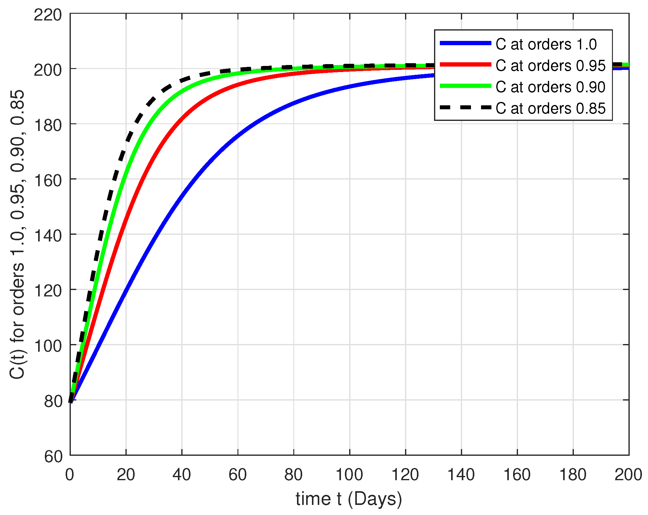
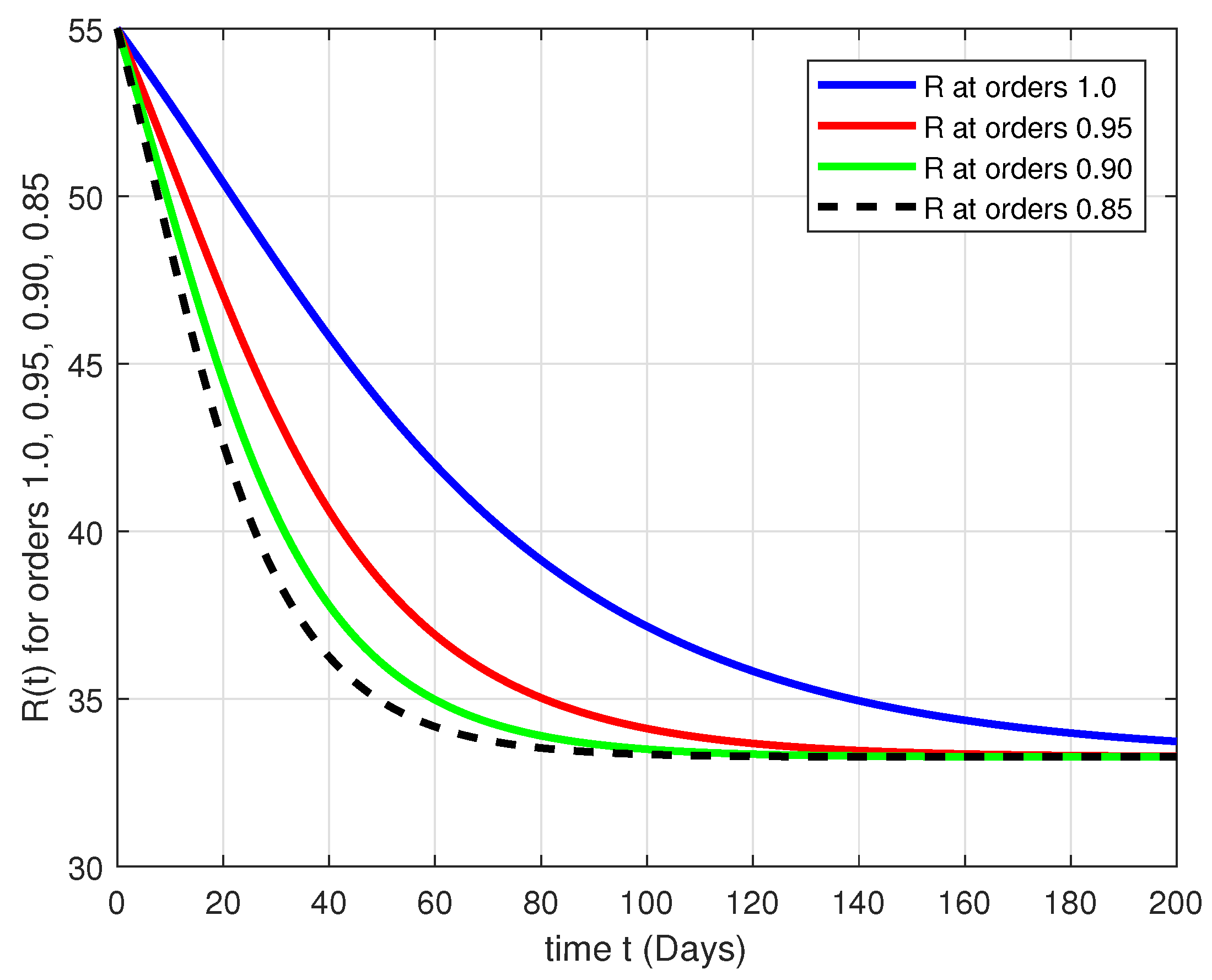
In this part, the numerical results about the fractal-fractional model (1) are provided with the help of our numerical scheme. The basic data were taken from the work given in [34]. We have: μ = 0.0001 , β = 0.0005 , α = 0.0002 , ρ 1 = 0.004 , ρ 2 = 0.002 , γ = 0.007 , λ = 0.9 , and the fractal fractional orders ν 1 , σ * = 1.0 , 0.95 , 0.90 , 0.85 .
In these figures, we can see the effect of fractal-fractional orders and dimensions on the numerical solutions of the given model. In Figure 1, by increasing the fractal-fractional orders and tending to the integer order, the slope of the graphs decrease, and after 120 days, all of them become stable. In Figure 2, the opposite of this happens. By increasing the fractal-fractional orders and tending to the integer order, the slope of the graphs is positive and it increases, and after 120 days, all of them become stable.
In Figure 3, we see the same behavior in the diagrams as in Figure 1. Finally, Figure 4 depicts an increase in the number of the quitter smokers by increasing the time, and all of the diagrams experience a slight slope by tending ν 1 , σ * to the integer-order.

8. Conclusions

In this article, we have studied a fractal-fractional order ice-smoking mathematical model (1) for the qualitative analysis and computational aspect. The qualitative work is based on the fixed-point approach, while the numerical simulations are obtained with the help of the Lagrange’s interpolation polynomial. For the numerical simulations, we analyzed the fractal-fractional order ice-smoking mathematical model (1) for the orders ν 1 = σ * = 1.0 , 0.95 , 0.90 , 0.85 . For further new development/continuation of the study on the subject area, we can use other fractional operators that have exponential decay type kernels for some new ideas.

Author Contributions

Conceptualization, A.S., H.K. and S.E.; formal analysis, H.K., M.D.l.S., J.A., C.T.D. and S.R.; funding acquisition, M.D.l.S.; methodology, A.S., J.A., S.E., C.T.D. and S.R.; and software, A.S., H.K. and S.E. All authors have read and agreed to the published version of the manuscript.

Funding

The third author is grateful to the Spanish Government and the European Commission for their support through grant RTI2018-094336-B-I00 (MCIU/AEI/FEDER, UE) and to the Basque Government for its support through grants IT1207-19 and IT1555-22.

Institutional Review Board Statement

Not applicable.

Informed Consent Statement

Not applicable.

Data Availability Statement

Data sharing is not applicable to this article as no datasets were generated or analyzed during the current study.

Acknowledgments

H.Khan and J. Alzabut are thankful to Prince Sultan University and OSTİM Technical University for their endless support. The fifth and seventh authors would like to thank Azarbaijan Shahid Madani University.

Conflicts of Interest

The authors declare no conflict of interest.

References

  1. McCoy, A. The Politics of Heroin in Southeast Asia; Harper and Row: New York, NY, USA, 1972. [Google Scholar]
  2. Cady, J.F. A History of Modern Burma; Cornell University Press: Ithaca, NY, USA, 1958. [Google Scholar]
  3. Khan, N.; Fahad, S. Review of Ice Drugs Utilization in Pakistan. 2019. Available online: https://ssrn.com/abstract=3511136 (accessed on 6 December 2022).
  4. Jenkins, P. “The ice age” the social construction of a drug panic. Justice Q. 1994, 11, 7–31. [Google Scholar] [CrossRef]
  5. Sharomi, O.; Gumel, A.B. Curtailing smoking dynamics: A mathematical modeling approach. Appl. Math. Comput. 2008, 195, 475–499. [Google Scholar] [CrossRef]
  6. Zaman, G. Qualitative behavior of giving up smoking models. Bull. Malays. Math. Sci. Soc. 2011, 34, 403–415. [Google Scholar]
  7. Swartz, J.B. Use of a multistage model to predict time trends in smoking induced lung cancer. J. Epidemiol. Community Health 1992, 46, 311–315. [Google Scholar] [CrossRef] [PubMed] [Green Version]
  8. Zeb, A.; Zaman, G.; Momani, S. Square-root dynamics of a giving up smoking model. Appl. Math. Model. 2013, 37, 5326–5334. [Google Scholar] [CrossRef]
  9. Huo, H.F.; Zhu, C.C. Influence of relapse in a giving up smoking model. Abstr. Appl. Anal. 2013, 2013, 525461. [Google Scholar] [CrossRef] [Green Version]
  10. Zeb, A.; Bano, A.; Alzahrani, E.; Zaman, G. Dynamical analysis of cigarette smoking model with a saturated incidence rate. AIP Adv. 2018, 8, 045317. [Google Scholar] [CrossRef]
  11. Zeb, A.; Hussain, S.; Algatani, O.J.; Zaman, G. Global aspects of age-structured cigarette smoking model. Mediterr. J. Math. 2018, 15, 72. [Google Scholar] [CrossRef]
  12. Haidong, Q.; Rahman, M.U.; Arfan, M. Fractional model of smoking with relapse and harmonic mean type incidence rate under Caputo operator. J. Appl. Math. Comput. 2022. [Google Scholar] [CrossRef]
  13. Singh, J.; Kumar, D.; Qurashi, M.A.; Baleanu, D. A new fractional model for giving up smoking dynamics. Adv. Differ. Equ. 2017, 2017, 88. [Google Scholar] [CrossRef] [Green Version]
  14. Khan, Z.A.; Rahman, M.U.; Shah, K. Study of a fractal-fractional smoking models with relapse and harmonic mean type incidence rate. J. Funct. Spaces 2021, 2021, 6344079. [Google Scholar] [CrossRef]
  15. Liu, C.; Sun, W.; Yi, X. Optimal control of a fractional smoking system. J. Ind. Manag. Opt. 2023, 19, 2936–2954. [Google Scholar] [CrossRef]
  16. Etemad, S.; Shikongo, A.; Owolabi, K.M.; Tellab, B.; Avci, I.; Rezapour, S.; Agarwal, R.P. A new fractal-fractional version of giving up smoking model: Application of Lagrangian piece-wise interpolation along with asymptotical stability. Mathematics 2022, 10, 4369. [Google Scholar] [CrossRef]
  17. Thaiprayoon, C.; Sudsutad, W.; Alzabut, J.; Etemad, S.; Rezapour, S. On the qualitative analysis of the fractional boundary valueproblem describing thermostat control model via ψ-Hilfer fractional operator. Adv. Differ. Equ. 2021, 2021, 201. [Google Scholar] [CrossRef]
  18. Rezapour, S.; Etemad, S.; Mohammadi, H. A mathematical analysis of a system of Caputo-Fabrizio fractional differential equationsfor the anthrax disease model in animals. Adv. Differ. Equ. 2020, 2020, 481. [Google Scholar] [CrossRef]
  19. Kumar, P.; Erturk, V.S.; Almusawa, H. Mathematical structure of mosaic disease using microbial biostimulants via Caputo and Atangana–Baleanu derivatives. Res. Phys. 2021, 24, 104186. [Google Scholar] [CrossRef]
  20. Asamoah, J.K.K.; Okyere, E.; Yankson, E.; Opoku, A.A.; Adom-Konadu, A.; Acheampong, E.; Arthur, Y.D. Non-fractional and fractional mathematical analysis and simulations for Q fever. Chaos Solitons Fractals 2022, 156, 111821. [Google Scholar] [CrossRef]
  21. Deressa, C.T.; Etemad, S.; Rezapour, S. On a new four-dimensional model of memristor-based chaotic circuit in the context of nonsingular Atangana–Baleanu-Caputo operators. Adv. Differ. Equ. 2021, 2021, 444. [Google Scholar] [CrossRef]
  22. Mohammadi, H.; Kumar, S.; Rezapour, S.; Etemad, S. A theoretical study of the Caputo-Fabrizio fractional modeling for hearing loss due to Mumps virus with optimal control. Chaos Solitons Fractals 2021, 144, 110668. [Google Scholar] [CrossRef]
  23. Khan, H.; Tunc, C.; Chen, W.; Khan, A. Existence theorems and Hyers–Ulam stability for a class of hybrid fractional differentialequations with p-Laplacial operator. J. Appl. Anal. Comput. 2018, 8, 1211–1226. [Google Scholar] [CrossRef]
  24. Kumar, P.; Erturk, V.S. Environmental persistence influences infection dynamics for a butterfly pathogen via new generalised Caputo type fractional derivative. Chaos Solitons Fractals 2021, 144, 110672. [Google Scholar] [CrossRef]
  25. Zarin, R.; Khaliq, H.; Khan, A.; Khan, D.; Akgul, A.; Humphries, U.W. Deterministic and fractional modeling of a computer virus propagation. Res. Phys. 2022, 33, 105130. [Google Scholar] [CrossRef]
  26. Wongcharoen, A.; Ntouyas, S.K.; Tariboon, J. Nonlocal boundary value problems for Hilfer type pantograph fractional differentialequations and inclusions. Adv. Differ. Equ. 2020, 2020, 279. [Google Scholar] [CrossRef]
  27. Amara, A.; Etemad, S.; Rezapour, S. Topological degree theory and Caputo-Hadamard fractional boundary value problems. Adv. Differ. Equ. 2020, 2020, 1–22. [Google Scholar] [CrossRef]
  28. Omame, A.; Nwajeri, U.K.; Abbas, M.; Onyenegecha, C.P. A fractional order control model for Diabetes and COVID-19 co-dynamics with Mittag–Leffler function. Alex. Eng. J. 2022, 61, 7619–7635. [Google Scholar] [CrossRef]
  29. Jafari, H.; Mahmoudi, M.; Skandari, M.H.N. A new numerical method to solve pantograph delay differential equations with convergence analysis. Adv. Differ. Equ. 2021, 2021, 129. [Google Scholar] [CrossRef]
  30. Rashid, S.; Kubra, K.T.; Jafari, H.; Lehre, S.U. A semi-analytical approach for fractional order Boussinesq equation in a gradient unconfined aquifers. Math. Methods Appl. Sci. 2022, 45, 1033–1062. [Google Scholar] [CrossRef]
  31. Omame, A.; Ele Isah, M.; Abbas, M.; Abdel-Aty, A.H.; Onyenegecha, C.P. A fractional order model for Dual Variants of COVID-19 and HIV co-infection via Atangana-Baleanu derivative. Alex. Eng. J. 2022, 61, 9715–9731. [Google Scholar] [CrossRef]
  32. Omame, A.; Abbas, M.; Onyenegecha, C.P. Backward bifurcation and optimal control in a co-infection model for SARS-CoV-2 and ZIKV. Res. Phys. 2022, 37, 105481. [Google Scholar] [CrossRef]
  33. Omame, A.; Abbas, M.; Abdel-Aty, A.H. Assessing the impact of SARS-CoV-2 infection on the dynamics of dengue and HIV via fractional derivatives. Chaos Solitons Fractals 2022, 162, 112427. [Google Scholar] [CrossRef]
  34. Zeb, A.; Alzahrani, A. Non-standard finite difference scheme and analysis of smoking model with reversion class. Res. Phys. 2021, 21, 103785. [Google Scholar] [CrossRef] [PubMed]
  35. Atangana, A. Fractal-fractional differentiation and integration: Connecting fractal calculus and fractional calculus to predict complex system. Chaos Solitons Fractals 2017, 102, 396–406. [Google Scholar] [CrossRef]
  36. Atangana, A.; Akgul, A.; Owolabi, K.M. Analysis of fractal fractional differential equations. Alex. Eng. J. 2020, 59, 1117–1134. [Google Scholar] [CrossRef]
Figure 1. Simulations for the S ( t ) class of the fractal-fractional model (1).
Symmetry 15 00087 g001
Figure 2. Simulations for the C ( t ) class of the fractal-fractional model (1).
Symmetry 15 00087 g002
Figure 3. Simulations for the R ( t ) class of the fractal-fractional model (1).
Symmetry 15 00087 g003
Figure 4. Simulations for the Q ( t ) of the fractal-fractional model (1).
Symmetry 15 00087 g004
Disclaimer/Publisher’s Note: The statements, opinions and data contained in all publications are solely those of the individual author(s) and contributor(s) and not of MDPI and/or the editor(s). MDPI and/or the editor(s) disclaim responsibility for any injury to people or property resulting from any ideas, methods, instructions or products referred to in the content.