Article

Multi-Criteria Decision-Making Method Based on Complex t-Spherical Fuzzy Aczel–Alsina Aggregation Operators and Their Application

1
Institute of Numerical Sciences, Kohat University of Science and Technology, Kohat 26000, KPK, Pakistan
2
Department of Mathematics, Deanship of Applied Sciences, Umm Al-Qura University, Makkah 24231, Saudi Arabia
*
Authors to whom correspondence should be addressed.
Symmetry 2023, 15(1), 85; https://doi.org/10.3390/sym15010085
Submission received: 30 November 2022 / Revised: 13 December 2022 / Accepted: 23 December 2022 / Published: 28 December 2022
(This article belongs to the Section Engineering and Materials)

Abstract

:
The complex t-spherical fuzzy set (Ct-SFS) is a potent tool for representing fuzziness and uncertainty compared to the picture fuzzy sets and spherical fuzzy sets. It plays a key role in modeling problems that require two-dimensional data. The present study purposes the aggregation technique of Ct-SFSs with the aid of Aczel–-Alsina (AA) operations. We first introduce certain novel AA operations of Ct-SFSs, such as the AA sum, AA product, AA scalar multiplication, and AA scalar power. Subsequently, we propound a series of complex t-spherical fuzzy averaging and geometric aggregation operators to efficiently aggregate complex t-spherical fuzzy data. In addition, we explore the different characteristics of these operators, discuss certain peculiar cases, and prove their fundamental results. Thereafter, we utilize these operators and propose entropy measures to frame a methodology for dealing with complex t-spherical fuzzy decision-making problems with unknown criteria weight data. Finally, we provide a case study about vehicle model selection to illustrate the presented method’s applicability followed by a parameter analysis and comparative study.

1. Introduction

The multi-criteria decision-making (MCDM) process is a skilled approach to handling complex and challenging inputs in realistic situations. MCDM is a process that generates rankings for available alternatives that correspond to the option’s distinct characteristic objects and is a critical component of decision-making sciences [1,2,3,4,5]. In real-world decision-making settings, it is vital to carry the characteristic object (well and precisely). Owing to the complexity and inability of decision-making situations, carrying the distinctive objects of options demands more than precise objects. Zadeh [6] presented a theory of fuzzy sets (FS) to achieve this, in which only the truth grade is confined to the unit interval. The FS theory has attracted extensive attention from notable experts and has been utilized in numerous scenarios in several sectors [7,8,9,10,11,12,13]. However, the FS doctrine has failed to function exactly in multiple instances. For example, it is hard to apply FS to details given in terms of truthfulness ( μ ) and falsity ( ν ) ratings. To solve these challenges, Atanassov [14] dispatched the theory of intuitionistic FS (IFS), a redesigned description of the FS that permits the effective handling of inconvenient and unreliable information. IFS includes grades μ and ν with the condition 0 μ + ν 1 . In contrast to an FS, an IFS examines both the amount of satisfaction and dissatisfaction in terms of membership and non-membership grades. Yager [15] recognized the limitations of IFSs; thus, he created the notion of Pythagorean FS (PyFS) by altering the IFS limitations with the rule 0 μ 2 + ν 2 1 . This new constraint states that the total squares of the membership and non-membership grades must be inside the unit interval, which widens the codomain. Likewise, Yager [16] once again recognized the restrictions in the assignments of grades to objects in PyFS; therefore, he introduced the concept of q-rung orthopair FS (q-ROFSs). q-ROFS includes the grades of membership μ and non-membership ν with the condition 0 μ q + ν q 1   ( q 1 ) . This set allows decision experts (DEs) to freely assign μ and ν by removing limits imposed by earlier set theories. Figure 1 displays the comparison of the IFS, PyFS, and q-ROFS ranges. The greatest area of the plane is covered by the curve of the q-ROFS for q = 8 ; this area increases when q is increased. Therefore, q-ROFS is regarded as the most credible generalization of FS. Wei et al. [17] devised the generalized Heronian mean operator, geometric Heronian mean operator and the corresponding weighted and hybrid forms under the q-rung orthopair fuzzy background. Shu et al. brought forward research on aggregating q-rung orthopair fuzzy continuous information [18]. Khan et al. [19] dispatched a graphical ranking technique and examined numerous examples with their proposed technique. Recently, J. Ali [20] criticized the existing score function and expanded measurements of alternatives and rankings according to the compromised solution (MARCOS) approach with unknown weight information to the context of q-rung orthopair fuzzy data based on the revised score function.
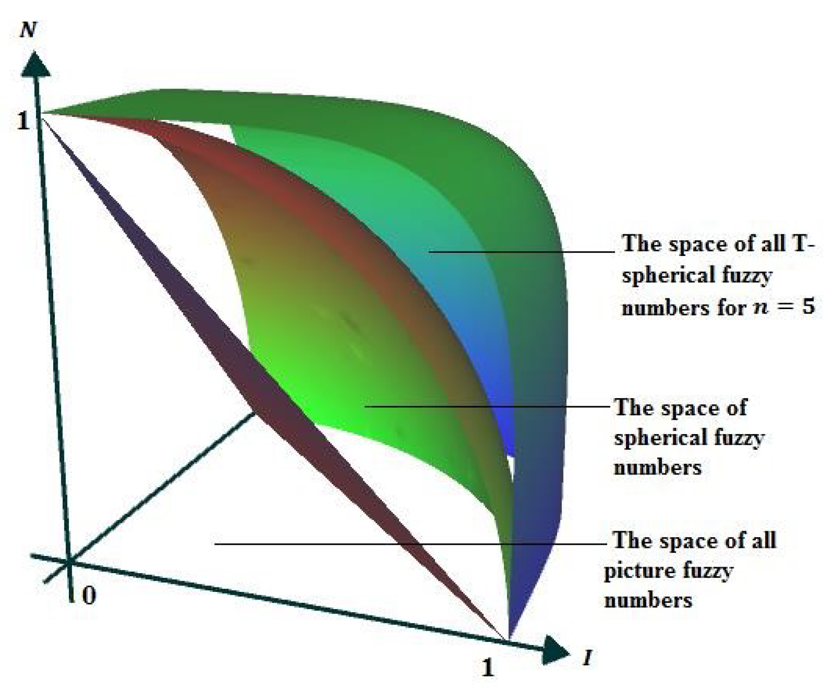
Later, the incorporation of abstinence grade ϑ led to the development of the concept of picture FS (PFS) by Cuong [21]. The grades for membership, abstinence, and non-membership were derived from the unit interval, such that the total of the three grades falls inside the fuzzy interval i.e., 0 μ + ϑ + ν 1 . PFS is constrained by the same constraints as IFS. Ullah et al. [22] developed the concept of spherical FS (SFS) by modifying the requirements as 0 μ 2 + ϑ 2 + ν 2 1 . In addition, Ullah et al. [22] propounded t-spherical FS (t-SFS) since PFS and SFS have constraints. In t-SFSs, the total membership, abstinence, and non-membership grades must be contained inside the unit interval when raised to the power t, i.e., 0 μ t + ϑ t + ν t 1 ( t 1 ) . t-SFS generalizes all prior set theories and is, thus, the most effective tool in the area. For instance, if μ , ϑ , and ν are, respectively, 0.3, 0.4, and 0.5, then PFS fails because the total is 1.2. However, SFS can handle such situations, as the sum of squares of three grades of SFS should fit within the unit interval. Again, SFS is restricted because it cannot handle situations in which μ , ϑ , and ν are, respectively, 0.8, 0.8, and 0.9. In such circumstances, the t-SFS is the most appropriate instrument since the grades may be raised by sufficiently large exponents, such that the aggregate falls inside the unit interval. In Figure 2, it is clearly shown that the t-SFS has a larger codomain in comparison to PFS and SFS. Gundogdu and Kahraman [23,24,25] investigated the SFSs and spherical fuzzy TOPSIS approach, the expansion of WASPAS with SFSs and spherical fuzzy hierarchy process, and its applications in the energy sector. Ullah and his collaborators [26] investigated Dombi aggregation operators by adding interval-valued t-SFS. Using the concept of t-spherical fuzzy graphs, Guleria and Bajaj [27] investigated two methodologies for solving decision-making problems. Mahnaz et al. [28] studied t-spherical fuzzy frank aggregation operators and outlined their relevant results at length. The authors of Reference [29] put forward an MCDM methodology on the basis of their initiated spherical fuzzy prioritized operators. Yang and Pang [30] recently developed t-spherical fuzzy Dombi Bonferroni mean operators and then applied them to solve the furniture procurement problem.
As stated before, FS paradigms are crucial modeling tools for uncertain and partial data. However, the FS paradigms suggested are insufficient to capture periodic data or two-dimensional phenomena. Ramot et al. [31,32] dispatched the notion of complex FS (CFS) to address this problem. The essence of Ramot’s concept is to expand the range of membership from [0, 1] to the complex plane’s unit circle. A CFS is defined by the membership function μ ¨ = μ e i 2 π ð μ , where μ is referred to as the amplitude term and takes values from the range [ 0 , 1 ] , and ð μ is referred to as the phase term (periodic term) and lies in the interval [ 0 , 1 ] . The phase term plays an essential part in establishing the CF model. This is what distinguishes the CF sets from other FS types and makes them outstanding. A CFS specifies the membership value of an element based on one amplitude and one phase term. In this regard, CFS is insufficient for modeling the non-membership grade. To circumvent this limitation, Alkouri and Salleh [33] developed complex intuitionistic FS (CIFS). Membership functions ( μ ¨ = μ e i 2 π ð μ ) and non-membership functions ( ν ¨ = ν e i 2 π ð ν ) are used to identify a CIFS, such that 0 μ + ν 1 and 0 ð μ + ð ν 1 . Rani and Garg [34] devised a decision-making method based on the distance between CIFSs. In addition, researchers examined the CIFS aggregation operator and decision-making methodologies [35,36,37]. As an extension of CIFSs, Ullah et al. [38] also presented the complex PFS (CPFS), which is defined by the membership function ( μ ¨ = μ e i 2 π ð μ ) , the neutral function ( ϑ ¨ = ϑ e i 2 π ð ϑ ) , and the non-membership function ( ν ¨ = ν e i 2 π ð ν ) under the constraints 0 μ + ϑ + ν 1 and 0 ð μ + ð ϑ + ð ν 1 as an expansion of CIFSs. Soon after, Ali et al. [39] identified the limitations of CPFS and originated the idea of complex t-SFS (Ct-SFS) with regard to the restrictions 0 μ t + ϑ t + ν t 1 and 0 ð μ t + ð ϑ t + ð ν t 1 , which is the generalization of complex SFS (CSFS) [40] and CPFS. Nasir et al. [41] established the concept of complex t-spherical fuzzy interactions and demonstrated several economic and international trade applications. Karaaslan and Dawood [42] highlighted the shortcomings of the ranking technique and defined innovative score and accuracy functions that are devoid of the problems identified. In Reference [43], the authors designed a series of complex t-spherical fuzzy power operators and tested their validity. Until now, various works related to Ct-SFSs have been explored by scholars but there is no study regarding criteria weight determination.
T-norm (TN) and T-cnorm (TCN) played crucial roles in the deployment of FSs in decision-making. Aczel and Alsina [44] first studied a new pair of TN and TCN that is more adaptable than the formerly designed TN and TCN. Wang et al. [45] developed a hybrid histogram equalization method based on the AA triangular norm that simultaneously widened the gap between forgers and authentic samples. In the field of decision-making frameworks, Senapati et al. [46,47] put forward AA aggregation operators for a framework of IFSs and interval-valued IFSs (IVIFSs), and then applied them to address MCDM issues, while Senapati [48] examined AA aggregation operators based on PFS with application to MCDM. In [49], the authors discussed picture fuzzy AA geometric aggregation information and used it to identify the factors influencing mango crops. A study by Ali and Naeem [50] provided certain AA complex q-rung orthopair fuzzy aggregation operators and put forward a novel entropy approach to overcome the defects of the existing entropy measures. Hussain et al. [51] diagnosed the fundamental t-spherical fuzzy aggregation operators in terms of AA operations. Simultaneously, Naeem and Ali [49] explored spherical fuzzy AA aggregation operators and their implications for solar energy cells. Recently, Mahmood et al. [52] studied the theory of bipolar complex fuzzy AA aggregation operators and their applications to MCDM problems. To our knowledge, no study has been conducted that combines the ideas of AA t-norm and t-conorm under the background of Ct-SFS. By exploiting the strengths of AA t-norm and t-conorm for offering flexibility in the decision-making procedure, it would be conceivable to originate a usable tool for executing a higher level of uncertainty in MCDM problems in a complex t-spherical fuzzy setting.

1.1. Motivations

Based on the discussion and literature analysis, it is evident that Ct-SFS is more effective than C-PFS and C-SFS in representing uncertain information when dealing with complex and uncertain choice situations. Although a substantial amount of research using C-TSFS has effectively supported decision analyses, some innovative aggregation theories, information measures, and decision approaches need to be investigated so that DEs can evaluate practical decision problems in a more comprehensive manner. From the published studies, the following are the motives for this study:
(i)
Aggregation-based decision algorithms provide DEs with easy and rapid methods for evaluating alternatives comprehensively. To incorporate complex t-spherical fuzzy data, it is, thus, required to provide practical and adaptable aggregation operators. The AA operations cannot only produce operations of Ct-SFNs but also include alternate parameters to make the decision analysis technique more versatile.
(ii)
The importance of criteria in decision analysis is very vital for acquiring rational decisions. However, most complex t-spherical fuzzy decision methodologies are based on the known weight of the criteria and ignore the determination of criteria weight. Therefore, it is necessary to explore a criteria-weight determination formulation to obtain more accurate results.

1.2. Contributions

In view of the aforementioned inspirations and discussion of the prevailing research, the main objective of this article is to propound a complex t-spherical fuzzy decision making methodology based on AA operations and the entropy measure to rank vehicle models. Complex t-spherical fuzzy AA operators were employed to aggregate DEs assessment information. Entropy was deployed to ascertain the objective weight of the criteria under a complex t-spherical fuzzy environment. Accordingly, the contributions of this research are enlisted as follows:
(i)
Initiate complex t-spherical fuzzy operational rules based on the AA t-norm and t-conorm and their accompanying results.
(ii)
Various innovative complex t-spherical fuzzy aggregation operators, such as a complex t-spherical fuzzy AA-weighted averaging operator, complex t-spherical fuzzy AA weighted geometric operator, and their corresponding order-weighted hybrid forms, are put forward on the basis of propounding operational rules to aggregate complex t-spherical fuzzy information; the related results of the expounded operators are also studied at length.
(iii)
Complex t-spherical fuzzy information entropy measure is proffered to measure to ascertain the objective weight of the criteria.
(iv)
A novel complex t-spherical fuzzy MCDM approach is built in light of the devised AA operators and the entropy measure formulation to address two-dimensional decision problems with unknown weight information.

1.3. Structure of This Research

To achieve the aims of our research, the remaining sections of this article are organized as follows: Section 2 provides a concise overview of the relevant background material for this article. Section 3 defines the AA operations of Ct-SFNs and verifies their essential properties. In Section 4, the theory of Ct-SFAAHWA and Ct-SFAAHWG operators are originated and we outline their influential characteristics with numerous strong results. Section 5 exploits the initiated operators to frame a decision-making algorithm for handling MCDM issues utilizing Ct-SFNs as characteristic values. In Section 6, a vehicle model selection problem is orated to demonstrate applicability, and a contrastive parameter analysis is conducted to highlight the stability of the framed approach. Section 7 includes a discussion regarding the results achieved from the application of the presented method. Some concluding remarks and future outlooks are documented at the end.

2. Preliminaries

In this section, we will introduce t-norm, t-conorm, AA t-norm, AA t-conorms, and some fundamental ideas of Ct-SFSs to aid readers in understanding the study.
Definition 1
([53]). A t-norm is a function T : 0 , 1 2 0 , 1 that satisfies
T1. 
T 1 , 2 = T 2 , 1 1 , 2 0 , 1 ;
T2. 
T 1 , 2 T 3 , 4 if 1 3 , 2 4 1 , 2 , 3 , 4 0 , 1 ;
T3. 
T , 1 = 0 , 1 ;
T4. 
T 1 , T 2 , 3 = T T 1 , 2 , 3 .
Some examples of t-norms
(1). 
T P 1 , 2 = 1 2 (product t-norm),
(2). 
T M 1 , 2 = min 1 , 2 (minimum t-norm),
(3). 
T L 1 , 2 = max 1 + 2 1 , 0 (Łukasiewicz t-norm),
(4). 
T D 1 , 2 = 1 , if   2 = 1 2 , if   1 = 1 ( drastic t-norm ) 0 , otherwise . 1 , 2 0 , 1 .
Definition 2
([54]). A t-conorm is a function S : 0 , 1 2 0 , 1 that satisfies
S1. 
S 1 , 2 = S 2 , 1 1 , 2 0 , 1 ;
S2. 
S 1 , 2 S 3 , 4 if 1 3 , 2 4 1 , 2 , 3 , 4 0 , 1 ;
S3. 
S , 0 = 0 , 1 ;
S4. 
S 1 , S 2 , 3 = S S 1 , 2 , 3 .
Some examples of t-conorms
(1). 
S P 1 , 2 = 1 + 2 1 2 (probabilistic sum),
(2). 
S M 1 , 2 = max 1 , 2 (maximum t-conorm),
(3). 
S L 1 , 2 = min 1 + 2 , 1 (Łukasiewicz t-conorm),
(4). 
S D 1 , 2 = 1 , if   2 = 0 2 , if   1 = 0 ( drastic t-conorm ) 1 , otherwise . 1 , 2 0 , 1 .
Moreover, ref. [54], when T is a t-norm and S is a t-conorm, then T 1 , 2 min 1 , 2 and S 1 , 2 max 1 , 2     1 , 2 0 , 1 .
Definition 3
([44]). The AA t-norm T A 0 , is described as
T A 1 , 2 = T D 1 , 2 , i f   = 0 min 1 , 2 , i f   = exp ln 1 + ln 2 1 / , o t h e r w i s e 1 , 2 0 , 1 .
Some special cases: T A = min , T A 0 = T D , T A 1 = T P .
Definition 4
([55]). The AA t-conorm S A 0 , is described as
S A 1 , 2 = S D 1 , 2 , i f   = 0 max 1 , 2 , i f   = 1 exp ln 1 1 + ln 1 2 1 / , o t h e r w i s e 1 , 2 0 , 1 .
Some special cases: S A = max , S A 0 = S D , S A 1 = S P .
The t-norm T A and t-conorm S A are dual with respect to each other 0 , . Furthermore, T A and S A are strictly increasing and strictly decreasing, respectively.
Only the AA category of t-norms fulfills the equivalence T A 1 § , 2 § = T A 1 , 2 § § > 0 and 1 , 2 0 , 1 .
In the following, we provide a concise overview of Ct-SFSs.
Definition 5.
A Ct-SFS ℑ on a fixed set X is characterized by
= , μ ¨ ( ) , ϑ ¨ ( ) , ν ¨ ( ) | X , t 1 ,
where μ ¨ ( ) = μ ( ) e i 2 π ð μ , ϑ ¨ ( ) = ϑ ( ) e i 2 π ð ϑ ,   ν ¨ ( ) = ν ( ) e i 2 π ð ν [ 0 , 1 ] marks the complex-valued membership, complex-valued neutral, and complex-valued non-membership grades of X , respectively; thus, 0 μ ( ) t + ϑ ( ) t + ν ( ) t 1 , 0 ð μ t + ð ϑ t + ð ν t 1 , where μ, ϑ, ν, ð μ , ð ϑ , ð ν 0 , 1 . The degree of hesitation is π t = 1 μ ( ) t + ϑ ( ) t + ν ( ) t 1 ð μ t + ð ϑ t + ð ν t . For convince, we termed = μ e i 2 π ð μ , ϑ e i 2 π ð ϑ , ν e i 2 π ð ν a complex t-spherical fuzzy number (Ct-SFN).
Definition 6
([42]). Let ℑ be a Ct-SFN, then the score function is characterized by:
S = 1 4 · 2 + μ t ϑ t ν t + ð μ t ð ϑ t ð ν t ,
where t [ 1 , ) , S 0 , 1 . The larger the value of S , the larger the Ct-SFN Q .
Definition 7
([42]). Let ℑ be a Ct-SFN, then the degree of accuracy is characterized as follows:
A = 1 4 · 2 + μ t + ϑ t + ν t + ð μ t + ð ϑ t + ð ν t ,
where A 0 , 1 . When the computed score values are similar, the larger the degree of accuracy A , the larger the Ct-SFN.
Definition 8.
Let 1 and 2 be any two Ct-SFNs and § > 0 , then their fundamental operational rules are described as follows:
1. 
1 2 = μ 1 t + μ 2 t μ 1 t μ 2 t 1 / t e i 2 π ð μ t 1 + ð μ t 2 ð μ t 1 ð μ t 2 1 / t , ϑ 1 ϑ 2 e i 2 π ð ϑ 1 ð ϑ 2 , ν 1 ν 2 e i 2 π ð ν 1 ð ν 2 ;
2. 
1 2 = μ 1 μ 2 e i 2 π ð μ 1 ð μ 2 , ϑ 1 t + ϑ 2 t ϑ 1 t ϑ 2 t 1 / t e i 2 π ð ϑ t 1 + ð ϑ t 2 ð ϑ t 1 ð ϑ t 2 1 / t , ν 1 t + ν 2 t ν 1 t ν 2 t 1 / t e i 2 π ð ν t 1 + ð ν t 2 ð ν t 1 ð ν t 2 1 / t ;
3. 
1 § = μ 1 § e i 2 π ð μ § 1 , 1 1 ϑ 1 t § 1 / t e i 2 π 1 1 ð ϑ t 1 § 1 / t , 1 1 ν 1 t § 1 / t e i 2 π 1 1 ð ν t 1 § 1 / t ;
4. 
§ 1 = 1 1 μ 1 t § 1 / t e i 2 π 1 1 ð μ t 1 § 1 / t , ϑ 1 § e i 2 π ð ϑ § 1 , ν 1 § e i 2 π ð ν § 1 ;
5. 
1 c = ν 1 e i 2 π ð ν 1 , ϑ 1 e i 2 π ð ϑ 1 , μ Q 1 e i 2 π ð μ 1 .

3. Complex t-Spherical Fuzzy AA Operational Laws

In light of Definitions 3 and 4, we now present some general operational laws for Ct-SFNs and their pertinent properties.
Definition 9.
Let 1 and 2 be any two Ct-SFNs, 1 and § > 0 , then the AA t-norm and t-conorm operations on them are characterized by
1. 
1 2 = 1 e ln 1 μ 1 t + ln 1 μ 2 t 1 / t e 2 i π 1 e ln 1 ð μ t 1 + ln 1 ð μ t 2 1 / t , e ln ϑ 1 t + ln ϑ 2 t 1 / t e 2 i π e ln ð ϑ t 1 + ln ð ϑ t 2 1 / t , e ln ν 1 t + ln ν 2 t 1 / t e 2 i π e ln ð ν t 1 + ln ð ν t 2 1 / t ;
2. 
1 2 = e ln μ 1 t + ln μ 2 t 1 / t e 2 i π e ln ð μ t 1 + ln ð μ t 2 1 / t , 1 e ln 1 ϑ 1 t + ln 1 ϑ 2 t 1 / t e 2 i π 1 e ln 1 ð ϑ t 1 + ln 1 ð ϑ t 2 1 / t , 1 e ln 1 ν 1 t + ln 1 ν 2 t 1 / t e 2 i π 1 e ln 1 ð ν t 1 + ln 1 ð ν t 2 1 / t ;
3. 
1 § = e § ln μ 1 t 1 / t e 2 i π e § ln ð μ t 1 1 / t , 1 e § ln 1 ϑ 1 t 1 / t e 2 i π 1 e § ln 1 ð ϑ t 1 1 / t , 1 e § ln 1 ν 1 t 1 / t e 2 i π 1 e § ln 1 ð ν t 1 1 / t , ;
4. 
§ 1 = 1 e § ln 1 μ 1 t 1 / t e 2 i π 1 e § ln 1 ð μ t 1 1 / t , e § ln ϑ 1 t 1 / t e 2 i π e § ln ð ϑ t 1 1 / t , e § ln ν 1 t 1 / t e 2 i π e § ln ð ν t 1 1 / t .
Theorem 1.
Let ℑ, 1 , and 2 be any three Ct-SFNs, then we have
1. 
1 2 = 2 1 ;
2. 
1 2 = 2 1 ;
3. 
§ 1 2 = § 1 § 2 , § > 0 ;
4. 
§ 1 + § 2 = § 1 § 2 , § 1 , § 2 > 0 ;
5. 
1 2 § = 1 § 2 § , § > 0 ;
6. 
§ 1 § 2 = § 1 + § 2 , § 1 , § 2 > 0 .
Proof. 
  • 1 2 = 1 e ln 1 μ 1 t + ln 1 μ 2 t 1 / t e 2 i π 1 e ln 1 ð μ t 1 + ln 1 ð μ t 2 1 / t , e ln ϑ 1 t + ln ϑ 2 t 1 / t e 2 i π e ln ð ϑ t 1 + ln ð ϑ t 2 1 / t , e ln ν 1 t + ln ν 2 t 1 / t e 2 i π e ln ð ν t 1 + ln ð ν t 2 1 / t = 1 e ln 1 μ 2 t + ln 1 μ 1 t 1 / t e 2 i π 1 e ln 1 ð μ t 2 + ln 1 ð μ t 1 1 / t , e ln ν 2 t + ln ν 1 t 1 / t e 2 i π e ln ð ϑ t 1 + ln ð ϑ t 1 1 / t , e ln ν 2 t + ln ν 1 t 1 / t e 2 i π e ln ð ν t 1 + ln ð ν t 1 1 / t = 2 1 .
  • 1 2 = e ln μ 1 t + ln μ 2 t 1 / t e 2 i π e ln ð μ t 1 + ln ð μ t 2 1 / t , 1 e ln 1 ϑ 1 t + ln 1 ϑ 2 t 1 / t e 2 i π 1 e ln 1 ð ϑ t 1 + ln 1 ð ϑ t 2 1 / t , 1 e ln 1 ν 1 t + ln 1 ν 2 t 1 / t e 2 i π 1 e ln 1 ð ν t 1 + ln 1 ð ν t 2 1 / t = e ln μ 2 t + ln μ 1 t 1 / t e 2 i π e ln ð μ t 2 + ln ð μ t 1 1 / t , 1 e ln 1 ϑ 2 t + ln 1 ϑ 1 t 1 / t e 2 i π 1 e ln 1 ð ϑ t 2 + ln 1 ð ϑ t 1 1 / t , 1 e ln 1 ν 2 t + ln 1 ν 1 t 1 / t e 2 i π 1 e ln 1 ð ν t 2 + ln 1 ð ν t 1 1 / t = 2 1 .
  • § 1 2 = 1 e § ln 1 μ 1 t + ln 1 μ 2 t 1 / t e 2 i π 1 e § ln 1 ð μ t 1 + ln 1 ð μ t 2 1 / t , e § ln ϑ 1 t + ln ϑ 2 t 1 / t e 2 i π e § ln ð ϑ t 1 + ln ð ϑ t 2 1 / t , e § ln ν 1 t + ln ν 2 t 1 / t e 2 i π e § ln ð ν t 1 + ln ð ν t 2 1 / t = 1 e § ln 1 μ 1 t 1 / t e 2 i π 1 e § ln 1 ð μ t 1 1 / t , e § ln ϑ 1 t 1 / t e 2 i π e § ln ð ϑ t 1 1 / t , e § ln ν 1 t 1 / t e 2 i π e § ln ð ν t 1 1 / t
    1 e § ln 1 μ 2 t 1 / t e 2 i π 1 e § ln 1 ð μ t 2 1 / t , e § ln ϑ 2 t 1 / t e 2 i π e § ln ð ϑ t 2 1 / t , e § ln ν 2 t 1 / t e 2 i π e § ln ð ν t 2 1 / t = § 1 § 2 .
  • § 1 § 2 = 1 e § 1 ln 1 μ t 1 / t e 2 i π 1 e § 1 ln 1 ð μ t 1 / t , e § 1 ln ϑ t 1 / t e 2 i π e § 1 ln ð ϑ t 1 / t , e § 1 ln ν t 1 / t e 2 i π e § 1 ln ð ν t 1 / t 1 e § 2 ln 1 μ t 1 / t e 2 i π 1 e § 2 ln 1 ð μ t 1 / t , e § 2 ln ϑ t 1 / t e 2 i π e § 2 ln ð ϑ t 1 / t , e § 2 ln ν t 1 / t e 2 i π e § 2 ln ð ν t 1 / t = 1 e ( § 1 + § 2 ) ln 1 μ t 1 / t e 2 i π 1 e ( § 1 + § 2 ) ln 1 ð μ t 1 / t , e ( § 1 + § 2 ) ln ϑ t 1 / t e 2 i π e ( § 1 + § 2 ) ln ð ϑ t 1 / t , e ( § 1 + § 2 ) ln ν t 1 / t e 2 i π e ( § 1 + § 2 ) ln ð ν t 1 / t = § 1 + § 2 .
  • 1 2 § = e ln μ 1 t + ln μ 2 t 1 / t e 2 i π e ln ð μ t 1 + ln ð μ t 2 1 / t , 1 e ln 1 ϑ 1 t + ln 1 ϑ 2 t 1 / t e 2 i π 1 e ln 1 ð ϑ t 1 + ln 1 ð ϑ t 2 1 / t , 1 e ln 1 ν 1 t + ln 1 ν 2 t 1 / t e 2 i π 1 e ln 1 ð ν t 1 + ln 1 ð ν t 2 1 / t § = e § ln μ 1 t + ln μ 2 t 1 / t e 2 i π e § ln ð μ t 1 + ln ð μ t 2 1 / t , 1 e § ln 1 ϑ 1 t + ln 1 ϑ 2 t 1 / t e 2 i π 1 e § ln 1 ð ϑ t 1 + ln 1 ð ϑ t 2 1 / t , 1 e § ln 1 ν 1 t + ln 1 ν 2 t 1 / t e 2 i π 1 e § ln 1 ð ν t 1 + ln 1 ð ν t 2 1 / t = e § ln μ 1 t 1 / t e 2 i π e § ln ð μ t 1 1 / t , 1 e § ln 1 ϑ 1 t 1 / t e 2 i π 1 e § ln 1 ð ϑ t 1 1 / t , 1 e § ln 1 ν 1 t 1 / t e 2 i π 1 e § ln 1 ð ν t 1 1 / t e § ln μ 2 t 1 / t e 2 i π e § ln ð μ t 2 1 / t , 1 e § ln 1 ϑ 2 t 1 / t e 2 i π 1 e § ln 1 ð ϑ t 2 1 / t , 1 e § ln 1 ν 2 t 1 / t e 2 i π 1 e § ln 1 ð ν t 2 1 / t = 1 § 2 § .
  • § 1 § 2 = e § 1 ln μ t 1 / t e 2 i π e § 1 ln ð μ t 1 / t , 1 e § 1 ln 1 ϑ t 1 / t e 2 i π 1 e § 1 ln 1 ð ϑ t 1 / t , 1 e § 1 ln 1 ν t 1 / t e 2 i π 1 e § 1 ln 1 ð ν t 1 / t e § 2 ln μ t 1 / t e 2 i π e § 2 ln ð μ t 1 / t , 1 e § 2 ln 1 ϑ t 1 / t e 2 i π 1 e § 2 ln 1 ð ϑ t 1 / t , 1 e § 2 ln 1 ν t 1 / t e 2 i π 1 e § 2 ln 1 ð ν t 1 / t = e ( § 1 + § 2 ) ln μ t 1 / t e 2 i π e ( § 1 + § 2 ) ln ð μ t 1 / t , 1 e ( § 1 + § 2 ) ln 1 ϑ t 1 / t e 2 i π 1 e ( § 1 + § 2 ) ln 1 ð ϑ t 1 / t , 1 e ( § 1 + § 2 ) ln 1 ν t 1 / t e 2 i π 1 e ( § 1 + § 2 ) ln 1 ð ν t 1 / t = § 1 + § 2 .

4. Complex t-Spherical Fuzzy AA Aggregation Operators and Theorems

This section describes some complex t-spherical fuzzy AA aggregation operators that are based on the arithmetic average operator and the geometric average operator.

4.1. Complex t-Spherical Fuzzy AA Averaging Aggregation Operators

Based on the proposed operations, in this section, we introduce some novel averaging aggregation operators, including complex t-spherical fuzzy AA average (Ct-SFAAA) operator, complex t-spherical fuzzy AA weighted averaging (Ct-SFAAWA) operator, complex t-spherical fuzzy AA ordered weighted averaging (Ct-SFAAOWA) operator, and complex t-spherical fuzzy AA hybrid averaging (Ct-SFAAHA) operator. In addition, particular cases and features of these operators are investigated.
Definition 10.
Let ι = μ ι e i 2 π ð μ ι , ϑ ι e i 2 π ð ϑ ι , ν ι e i 2 π ð ν ι ι = 1 , 2 , , be a series of Ct-SFNs, then the Ct-SFAAWA operator is:
C t S F A A W A 1 , 2 , , = ι = 1 ⨿ ι ι ,
where ⨿ = ⨿ 1 , ⨿ 2 , , ⨿ T is the weight vector of ι ι = 1 , 2 , , such that ⨿ ι > 0 and ι = 1 ⨿ ι = 1 . Peculiarly, if ⨿ = 1 , 1 , , 1 T , then the Ct-SFAAWA operator is then reduced to the Ct-SFAAA operator of dimension ℏ, which is detailed below:
C t S F A A A 1 , 2 , , = 1 ι = 1 ι .
Theorem 2.
Let ι = μ ι e 2 i π ð μ ι , ϑ ι e 2 i π ð ϑ ι , ν ι e 2 i π ð ν ι ι = 1 , 2 , , be a series of Ct-SFNs, then the result obtained by utilizing the Ct-SFAAWA operator is still a Ct-SFN, and
C t S F A A W A 1 , 2 , , = 1 e ι = 1 ⨿ ι ln 1 μ ι t 1 / t e 2 i π 1 e ι = 1 ⨿ ι ln 1 ð μ t ι 1 / t , e ι = 1 ⨿ ι ln ϑ ι t 1 / t e 2 i π e ι = 1 ⨿ ι ln ð ϑ t ι 1 / t , e ι = 1 ⨿ ι ln ν ι t 1 / t e 2 i π e ι = 1 ⨿ ι ln ð ν t ι 1 / t .
Proof. 
Using the mathematical induction method, we can demonstrate Theorem 2 in the following way:
For = 2 , we have
C t S F A A W A 1 , 2 = ⨿ 1 1 ⨿ 2 2 = 1 e ⨿ 1 ln 1 μ 1 t 1 / t e 2 i π 1 e ⨿ 1 ln 1 ð μ t 1 1 / t , e ⨿ 1 ln ϑ 1 t 1 / t e 2 i π e ⨿ 1 ln ð ϑ t 1 1 / t , e ⨿ 1 ln ν 1 t 1 / t e 2 i π e ⨿ 1 ln ð ν t 1 1 / t 1 e ⨿ 2 ln 1 μ 2 t 1 / t e 2 i π 1 e ⨿ 2 ln 1 ð μ t 2 1 / t , e ⨿ 2 ln ϑ 2 t 1 / t e 2 i π e ⨿ 2 ln ð ϑ t 2 1 / t , e ⨿ 2 ln ν 2 t 1 / t e 2 i π e ⨿ 2 ln ð ν t 2 1 / t = 1 e ⨿ 1 ln 1 μ 1 t + ⨿ 2 ln 1 μ 2 t 1 / t e 2 i π 1 e ⨿ 1 ln 1 ð μ t 1 + ⨿ 2 ln 1 ð μ t 2 1 / t , e ⨿ 1 ln ϑ 1 t + ⨿ 2 ln ϑ 2 t 1 / t e 2 i π e ⨿ 1 ln ð ϑ t 1 + ⨿ 2 ln ð ϑ t 2 1 / t , e ⨿ 1 ln ν 1 t + ⨿ 2 ln ν 2 t 1 / t e 2 i π e ⨿ 1 ln ð ν t 1 + ⨿ 2 ln ð ν t 2 1 / t = 1 e ι = 1 2 ⨿ ι ln 1 μ ι t 1 / t e 2 i π 1 e ι = 1 2 ⨿ ι ln 1 ð μ t ι 1 / t , e ι = 1 2 ⨿ ι ln ϑ ι t 1 / t e 2 i π e ι = 1 2 ⨿ ι ln ð ϑ t ι 1 / t , e ι = 1 2 ⨿ ι ln ν ι t 1 / t e 2 i π e ι = 1 2 ⨿ ι ln ð ν t ι 1 / t .
Hence, the result is true for = 2 .
Suppose that Equation (8) is true for = k , then we have
C t S F A A W A 1 , 2 , , k = ι = 1 k ⨿ ι ι = 1 e ι = 1 k ⨿ ι ln 1 μ ι t 1 / t e 2 i π 1 e ι = 1 k ⨿ ι ln 1 ð μ t ι 1 / t , e ι = 1 k ⨿ ι ln ϑ ι t 1 / t e 2 i π e ι = 1 k ⨿ ι ln ð ϑ t ι 1 / t , e ι = 1 k ⨿ ι ln ν ι t 1 / t e 2 i π e ι = 1 k ⨿ ι ln ð ν t ι 1 / t
Now for = k + 1 , we have
C t S F A A W A 1 , 2 , , k , k + 1 = ι = 1 k ⨿ ι ι ⨿ k + 1 k + 1 = 1 e ι = 1 k ⨿ ι ln 1 μ ι t 1 / t e 2 i π 1 e ι = 1 k ⨿ ι ln 1 ð μ t ι 1 / t , e ι = 1 k ⨿ ι ln ϑ ι t 1 / t e 2 i π e ι = 1 k ⨿ ι ln ð ϑ t ι 1 / t , e ι = 1 k ⨿ ι ln ν ι t 1 / t e 2 i π e ι = 1 k ⨿ ι ln ð ν t ι 1 / t 1 e ⨿ k + 1 ln 1 μ k + 1 t 1 / t e 2 i π 1 e ⨿ k + 1 ln 1 ð μ t k + 1 1 / t , e ⨿ k + 1 ln ϑ k + 1 t 1 / t e 2 i π e ⨿ k + 1 ln ϑ k + 1 t 1 / t , e ⨿ k + 1 ln ν k + 1 t 1 / t e 2 i π e ⨿ k + 1 ln ν k + 1 t 1 / t = 1 e ι = 1 k + 1 ⨿ ι ln 1 μ ι t 1 / t e 2 i π 1 e ι = 1 k + 1 ⨿ ι ln 1 ð μ t ι 1 / t , e ι = 1 k + 1 ⨿ ι ln ϑ ι t 1 / t e 2 i π e ι = 1 k + 1 ⨿ ι ln ð ϑ t ι 1 / t , e ι = 1 k + 1 ⨿ ι ln ν ι t 1 / t e 2 i π e ι = 1 k + 1 ⨿ ι ln ð ν t ι 1 / t .
Thus, Equation (8) is legitimate for = k + 1 and, hence, by the principle of mathematical induction, the result given in Equation (8) is true for all positive integers . □
Theorem 3.
(Idempotency) Let ι = μ ι e 2 i π ð μ ι , ϑ ι e 2 i π ð ϑ ι , ν ι e 2 i π ð ν ι ι = 1 , 2 , , be a series of Ct-SFNs, if ι = ι , then
C t S F A A W A 1 , 2 , , = .
Proof. 
Since ι = ι , and ι = 1 ⨿ ι = 1 so by Theorem 2, we have
C t S F A A W A 1 , 2 , , = 1 e ι = 1 ⨿ ι ln 1 μ t 1 / t e 2 i π 1 e ι = 1 ⨿ ι ln 1 ð μ t 1 / t , e ι = 1 ⨿ ι ln ϑ t 1 / t e 2 i π e ι = 1 ⨿ ι ln ð ϑ t 1 / t , e ι = 1 ⨿ ι ln ν t 1 / t e 2 i π e ι = 1 ⨿ ι ln ð ν t 1 / t = 1 e ln 1 μ t 1 / t e 2 i π 1 e ln 1 ð μ t 1 / t , e ln ϑ t 1 / t e 2 i π e ln ð ϑ t 1 / t , e ln ν t 1 / t e 2 i π e ln ð ν t 1 / t = μ e 2 i π ð μ , ϑ e 2 i π ð ϑ , ν e 2 i π ð ν = .
Theorem 4
(Monotonicity). Let ι = μ ι e 2 i π ð μ ι , ϑ ι e 2 i π ð ϑ ι , ν ι e 2 i π ð ν ι ι = 1 , 2 , , and ˙ ι = μ ˙ ι e 2 i π ð μ ˙ ι , ϑ ˙ ι e 2 i π ð ϑ ˙ ι , ν ˙ ι e 2 i π ð ν ˙ ι ι = 1 , 2 , , be two series of Ct-SFNs, such that μ ι e 2 i π ð μ ι μ ˙ ι e 2 i π ð μ ˙ ι   ϑ ι e 2 i π ð ϑ ι ϑ ˙ ι e 2 i π ð ϑ ˙ ι and ν ι e 2 i π ð ν ι ν ˙ ι e 2 i π ð ν ˙ ι ι , then
C t S F A A W A 1 , 2 , , C t S F A A W A ˙ 1 , ˙ 2 , , ˙ .
Proof. 
Since μ ι e 2 i π ð μ ι μ ˙ ι e 2 i π ð μ ˙ ι ,   ϑ ι e 2 i π ð ϑ ι ϑ ˙ ι e 2 i π ð ϑ ˙ ι and ν ι e 2 i π ð ν ι ν ˙ ι e 2 i π ð ν ˙ ι ι . Accordingly, we have the following inequalities,
1 e ι = 1 ⨿ ι ln 1 μ ι t 1 / t e 2 i π 1 e ι = 1 ⨿ ι ln 1 ð μ t ι 1 / t 1 e ι = 1 ⨿ ι ln 1 μ ˙ ι t 1 / t e 2 i π 1 e ι = 1 ⨿ ι ln 1 ð μ ˙ t ι 1 / t , e ι = 1 ⨿ ι ln ϑ ι t 1 / t e 2 i π e ι = 1 ⨿ ι ln ð ϑ t ι 1 / t e ι = 1 ⨿ ι ln ϑ ˙ ι t 1 / t e 2 i π e ι = 1 ⨿ ι ln ð ϑ t ι 1 / t
and
e ι = 1 ⨿ ι ln ν ι t 1 / t e 2 i π e ι = 1 ⨿ ι ln ð ν t ι 1 / t e ι = 1 ⨿ ι ln ν ˙ ι t 1 / t e 2 i π e ι = 1 ⨿ ι ln ð ν t ι 1 / t
which implies that
1 e ι = 1 ⨿ ι ln 1 μ ι t 1 / t e 2 i π 1 e ι = 1 ⨿ ι ln 1 ð μ t ι 1 / t , e ι = 1 ⨿ ι ln ϑ ι t 1 / t e 2 i π e ι = 1 ⨿ ι ln ð ϑ t ι 1 / t , e ι = 1 ⨿ ι ln ν ι t 1 / t e 2 i π e ι = 1 ⨿ ι ln ð ν t ι 1 / t 1 e ι = 1 ⨿ ι ln 1 μ ˙ ι t 1 / t e 2 i π 1 e ι = 1 ⨿ ι ln 1 ð μ ˙ t ι 1 / t , e ι = 1 ⨿ ι ln ϑ ˙ ι t 1 / t e 2 i π e ι = 1 ⨿ ι ln ð ϑ ˙ t ι 1 / t , e ι = 1 ⨿ ι ln ν ˙ ι t 1 / t e 2 i π e ι = 1 ⨿ ι ln ð ν ˙ t ι 1 / t
Hence C t S F A A W A 1 , 2 , , C t S F A A W A ˙ 1 , ˙ 2 , , ˙ . □
Theorem 5
(Boundedness). Let ι = μ ι e 2 i π ð μ ι , ϑ ι e 2 i π ð ϑ ι , ν ι e 2 i π ð ν ι ι = 1 , 2 , , be a series of Ct-SFNs, and let = min 1 , 2 , , and + = max 1 , 2 , , , then
C t S F A A W A 1 , 2 , , + .
Proof. 
As given that
= min 1 , 2 , , = μ e 2 i π ð μ , ϑ e 2 i π ð ϑ , ν e 2 i π ð ν
and
+ = max 1 , 2 , , = μ + e 2 i π ð μ + , ϑ + e 2 i π ð ϑ + , ν + e 2 i π ð ν + ,
where
μ e 2 i π ð μ = min μ 1 e 2 i π ð μ 1 , μ 2 e 2 i π ð μ 2 , , μ e 2 i π ð μ ,
ϑ e 2 i π ð ϑ = max ϑ 1 e 2 i π ð ϑ 1 , ϑ 2 e 2 i π ð ϑ 2 , , ϑ e 2 i π ð ϑ ,
ν e 2 i π ð ν = max ν 1 e 2 i π ð ν 1 , ν 2 e 2 i π ð ν 2 , , ν e 2 i π ð μ ,
μ + e 2 i π ð μ + = max μ 1 e 2 i π ð μ 1 , μ 2 e 2 i π ð μ 2 , , μ e 2 i π ð μ ,
ϑ + e 2 i π ð ϑ + = min ϑ 1 e 2 i π ð ϑ 1 , ϑ 2 e 2 i π ð ϑ 2 , , ϑ e 2 i π ð ϑ
and
ν + e 2 i π ð ν + = min ν 1 e 2 i π ð ν 1 , ν 2 e 2 i π ð ν 2 , , ν e 2 i π ð ν .
As a result, there are ongoing inequities:
1 e ι = 1 ⨿ ι ln 1 μ t 1 / t e 2 i π 1 e ι = 1 ⨿ ι ln 1 ð μ t 1 / t 1 e ι = 1 ⨿ ι ln 1 μ ι t 1 / t e 2 i π 1 e ι = 1 ⨿ ι ln 1 ð μ t ι 1 / t 1 e ι = 1 ⨿ ι ln 1 μ + t 1 / t e 2 i π 1 e ι = 1 ⨿ ι ln 1 ð μ + t 1 / t
e ι = 1 ⨿ ι ln ϑ + t 1 / t e 2 i π e ι = 1 ⨿ ι ln ð ϑ + t 1 / t e ι = 1 ⨿ ι ln ϑ ι t 1 / t e 2 i π e ι = 1 ⨿ ι ln ð ϑ t ι 1 / t e ι = 1 ⨿ ι ln ϑ t 1 / t e 2 i π e ι = 1 ⨿ ι ln ð ϑ t 1 / t
e ι = 1 ⨿ ι ln ν + t 1 / t e 2 i π e ι = 1 ⨿ ι ln ð ν + t 1 / t e ι = 1 ⨿ ι ln ν ι t 1 / t e 2 i π e ι = 1 ⨿ ι ln ð ν t ι 1 / t e ι = 1 ⨿ ι ln ν t 1 / t e 2 i π e ι = 1 ⨿ ι ln ð ν t 1 / t .
Thereby, C t S F A A W A 1 , 2 , , + . □
Theorem 6
(Symmetry). Let ι = μ ι e 2 i π ð μ ι , ϑ ι e 2 i π ð ϑ ι , ν ι e 2 i π ð ν ι ι = 1 , 2 , , be a series of Ct-SFNs. Then, if ˘ ι = μ ˘ ι e 2 i π ð μ ˘ ι , ϑ ˘ ι e 2 i π ð ϑ ˘ ι , ν ˘ ι e 2 i π ð ν ˘ ι ι = 1 , 2 , , be any permutation of ι , then we have
C t S F A A W A 1 , 2 , , = C t S F A A W A ˘ 1 , ˘ 2 , , ˘ .
Proof. 
The proof is obvious and, thus, omitted. □
Next, we introduce the complex t-spherical fuzzy AA ordered-weighted averaging (Ct-SFAAOWA) operator.
Definition 11.
Let ι = μ ι e 2 i π ð μ ι , ϑ ι e 2 i π ð ϑ ι , ν ι e 2 i π ð ν ι ι = 1 , 2 , , be a series of Ct-SFNs, then the Ct-SFAAOWA operator is:
C t S F A A O W A 1 , 2 , , = ι = 1 ϖ ι δ ( ι ) ,
where ϖ = ϖ 1 , ϖ 2 , , ϖ T is the position weights of ι ι = 1 , 2 , , such that ϖ ι > 0 and ι = 1 ϖ ι = 1 . δ ( 1 ) , δ ( 2 ) , , δ ( ) is a permutation of 1 , 2 , , such that δ ( ι 1 ) δ ( ι ) for ι = 1 , 2 , , .
Theorem 7.
Let ι = μ ι e 2 i π ð μ ι , ϑ ι e 2 i π ð ϑ ι , ν ι e 2 i π ð ν ι ι = 1 , 2 , , be a series of Ct-SFNs, then the result obtained by utilizing the Ct-SFAAOWA operator is still a Ct-SFN, and
C t S F A A O W A 1 , 2 , , = 1 e ι = 1 ϖ ι ln 1 μ δ ( ι ) t 1 / t e 2 i π 1 e ι = 1 ϖ ι ln 1 ð μ t δ ( ι ) 1 / t , e ι = 1 ϖ ι ln ϑ δ ( ι ) t 1 / t e 2 i π e ι = 1 ϖ ι ln ð ϑ t δ ( ι ) 1 / t , e ι = 1 ϖ ι ln ν δ ( ι ) t 1 / t e 2 i π e ι = 1 ϖ ι ln ð ν t δ ( ι ) 1 / t .
Proof. 
We omit the verification of this theorem because it is identical to the proof of Theorem 2. □
The following characteristics can be presented successfully with the Ct-SFAAOWA operator.
Theorem 8
(Idempotency). Let ι = μ ι e 2 i π ð μ ι , ϑ ι e 2 i π ð ϑ ι , ν ι e 2 i π ð ν ι ι = 1 , 2 , , be a series of Ct-SFNs, if ι = ι , then
C t S F A A O W A 1 , 2 , , = .
Theorem 9
(Monotonicity). Let ι = μ ι e 2 i π ð μ ι , ϑ ι e 2 i π ð ϑ ι , ν ι e 2 i π ð ν ι ι = 1 , 2 , , and ˙ ι = μ ˙ ι e 2 i π ð μ ˙ ι , ϑ ˙ ι e 2 i π ð ϑ ˙ ι , ν ˙ ι e 2 i π ð ν ˙ ι ι = 1 , 2 , , be two series of Ct-SFNs, such that μ ι e 2 i π ð μ ι μ ˙ ι e 2 i π ð μ ˙ ι , ϑ ι e 2 i π ð ϑ ι ϑ ˙ ι e 2 i π ð ϑ ˙ ι and ν ι e 2 i π ð ν ι ν ˙ ι e 2 i π ð ν ˙ ι ι , then
C t S F A A O W A 1 , 2 , , C t S F A A O W A ˙ 1 , ˙ 2 , , ˙ .
Theorem 10
(Boundedness). Let ι = μ ι e 2 i π ð μ ι , ϑ ι e 2 i π ð ϑ ι , ν ι e 2 i π ð ν ι ι = 1 , 2 , , be a series of Ct-SFNs, and let = min 1 , 2 , , and + = max 1 , 2 , , , then
C t S F A A O W A 1 , 2 , , + .
Theorem 11
(Symmetry). Let ι = μ ι e 2 i π ð μ ι , ϑ ι e 2 i π ð ϑ ι , ν ι e 2 i π ð ν ι ι = 1 , 2 , , be a series of Ct-SFNs. Then, if ˘ ι = μ ˘ ι e 2 i π ð μ ˘ ι , ϑ ˘ ι e 2 i π ð ϑ ˘ ι , ν ˘ ι e 2 i π ð ν ˘ ι ι = 1 , 2 , , be any permutation of ι , then we have
C t S F A A W A 1 , 2 , , = C t S F A A W A ˘ 1 , ˘ 2 , , ˘ .
The Ct-SFAAWA operator weighs just the Ct-SFNs, as defined by Definition 10, while the Ct-SFAAOWA operator weighs only the ordered locations of the Ct-SFNs, as defined by Definition 11. As a result, weights represent various aspects of the Ct-SFAAWA and Ct-SFAAOWA operators. Nonetheless, one of the operators, as well as the other operators, consider just one of them. To address this shortcoming, we study the complex t-spherical fuzzy AA hybrid averaging (Ct-SFAAHA) operator, which weights all of the provided Ct-SFN and their appropriate ordered positions.
Definition 12.
Let ι = μ ι e 2 i π ð μ ι , ϑ ι e 2 i π ð ϑ ι , ν ι e 2 i π ð ν ι ι = 1 , 2 , , be a series of Ct-SFNs, then the Ct-SFAAHA operator is:
C t S F A A H A 1 , 2 , , = ι = 1 ϖ ι ^ δ ( ι ) ,
where ϖ = ϖ 1 , ϖ 2 , , ϖ T is the weight vector associated with Ct-SFAAHA ι ι = 1 , 2 , , such that ϖ ι > 0 and ι = 1 ϖ ι = 1 , ⨿ = ⨿ 1 , ⨿ 2 , , ⨿ T is the weight vector of ι ι = 1 , 2 , , such that ⨿ ι > 0 and ι = 1 ⨿ ι = 1 .   ^ δ ( ι ) is the ιth largest of the weighted Ct-SFNs ^ ι ^ ι = ⨿ ι ι , ι = 1 , 2 , , and ℏ is the balancing coefficient.
Theorem 12.
Let ι = μ ι e 2 i π ð μ ι , ϑ ι e 2 i π ð ϑ ι , ν ι e 2 i π ð ν ι ι = 1 , 2 , , be a series of Ct-SFNs, then the result acquired by using the Ct-SFAAHA operator is still a Ct-SFN, and
C t S F A A H A 1 , 2 , , = 1 e ι = 1 ϖ ι ln 1 μ ^ δ ( ι ) t 1 / t e 2 i π 1 e ι = 1 ϖ ι ln 1 ð μ ^ t δ ( ι ) 1 / t , e ι = 1 ϖ ι ln ϑ ^ δ ( ι ) t 1 / t e 2 i π e ι = 1 ϖ ι ln ð ϑ ^ t δ ( ι ) 1 / t , e ι = 1 ϖ ι ln ν ^ δ ( ι ) t 1 / t e 2 i π e ι = 1 ϖ ι ln ð ν ^ t δ ( ι ) 1 / t .
Proof. 
We omit the verification of this theorem because it is identical to the proof of Theorem 2. □
Similarly to the Ct-SFAAWA and Ct-SFAAOWA operators, the Ct-SFAAHA operator follows the properties of idempotency, monotonicity, boundedness, and symmetry. In addition to the aforementioned characteristics, the Ct-SFAAHA operator has the following special cases.
Corollary 1.
The Ct-SFAAWA operator is a special case of the Ct-SFAAHA operator.
Proof. 
Let ϖ = 1 , 1 , , 1 T , then
C t S F A A H A 1 , 2 , , = ϖ 1 ^ δ ( 1 ) ϖ 2 ^ δ ( 2 ) ϖ ^ δ ( ) = 1 ^ δ ( 1 ) ^ δ ( 2 ) ^ δ ( ) = ⨿ 1 1 ⨿ 2 2 ⨿ = C t S F A A W A 1 , 2 , , .
Corollary 2.
The Ct-SFAAOWA operator is a special case of the Ct-SFAAHA operator.
Proof. 
Let ⨿ = 1 , 1 , , 1 T , then
C t S F A A H A 1 , 2 , , = ϖ 1 ^ δ ( 1 ) ϖ 2 ^ δ ( 2 ) ϖ ^ δ ( ) = ϖ 1 δ ( 1 ) ϖ 2 δ ( 2 ) ϖ δ ( ) = C t S F A A O W A 1 , 2 , , .

4.2. Complex t-Spherical Fuzzy AA Geometric Aggregation Operators

Based on the proposed operations, in this subsection, we present some new geometric aggregation operators including complex t-spherical fuzzy AA geometric (Ct-SFAAG) operator, complex t-spherical fuzzy AA weighted geometric (Ct-SFAAWG) operator, complex t-spherical fuzzy AA order-weighted geometric (Ct-SFAAOWG) operator, and the complex t-spherical fuzzy AA hybrid geometric (Ct-SFAAHG) operator. Additionally, we investigate some special cases and characteristics of these operators.
Definition 13.
Let ι = μ ι e 2 i π ð μ ι , ϑ ι e 2 i π ð ϑ ι , ν ι e 2 i π ð ν ι ι = 1 , 2 , , be a series of Ct-SFNs, then the Ct-SFAAWG operator is:
C t S F A A W G 1 , 2 , , = ι = 1 ι ⨿ ι ,
where ⨿ = ⨿ 1 ,   ⨿ 2 , , ⨿ T is the weight vector of ι ι = 1 , 2 , , such that ⨿ ι > 0 and ι = 1 ⨿ ι = 1 . peculiarly, if ⨿ = 1 , 1 , , 1 T , then the Ct-SFAAWG operator reduces to the Ct-SFAAG operator of dimension ℏ, described as follows:
C t S F A A G 1 , 2 , , = ι = 1 ι 1 .
Theorem 13.
Let ι = μ ι e 2 i π ð μ ι , ϑ ι e 2 i π ð ϑ ι , ν ι e 2 i π ð ν ι ι = 1 , 2 , , be a series of Ct-SFNs, then the result acquired by using the Ct-SFAAWG operator are still Ct-SFN, and
C t S F A A W G 1 , 2 , , = e ι = 1 ⨿ ι ln μ ι t 1 / t e 2 i π e ι = 1 ⨿ ι ln ð μ t ι 1 / t , 1 e ι = 1 ⨿ ι ln 1 ϑ ι t 1 / t e 2 i π 1 e ι = 1 ⨿ ι ln 1 ð ϑ t ι 1 / t , 1 e ι = 1 ⨿ ι ln 1 ν ι t 1 / t e 2 i π 1 e ι = 1 ⨿ ι ln 1 ð ν t ι 1 / t .
Proof. 
We can verify Theorem 13 using the mathematical induction approach in the following way:
For = 2 , we have
C t S F A A W G 1 , 2 = 1 ⨿ 1 2 ⨿ 2 = e ⨿ 1 ln μ 1 t 1 / t e 2 i π e ⨿ 1 ln ð μ t 1 1 / t , 1 e ⨿ 1 ln 1 ϑ 1 t 1 / t e 2 i π 1 e ⨿ 1 ln 1 ð ϑ t 1 1 / t , 1 e ⨿ 1 ln 1 ν 1 t 1 / t e 2 i π 1 e ⨿ 1 ln 1 ð ν t 1 1 / t e ⨿ 2 ln μ 2 t 1 / t e 2 i π e ⨿ 2 ln ð μ t 2 1 / t , 1 e ⨿ 2 ln 1 ϑ 2 t 1 / t e 2 i π 1 e ⨿ 2 ln 1 ð ϑ t 2 1 / t , 1 e ⨿ 2 ln 1 ν 2 t 1 / t e 2 i π 1 e ⨿ 2 ln 1 ð ν t 2 1 / t = e ⨿ 1 ln μ 1 t + ⨿ 2 ln ν 2 t 1 / t e 2 i π e ⨿ 1 ln ð μ t 1 + ⨿ 2 ln ν 2 t 1 / t , 1 e ⨿ 1 ln 1 ϑ 1 t + ⨿ 2 ln 1 ϑ 2 t 1 / t e 2 i π 1 e ⨿ 1 ln 1 ð ϑ t 1 + ⨿ 2 ln 1 ϑ 2 t 1 / t , 1 e ⨿ 1 ln 1 ν 1 t + ⨿ 2 ln 1 ν 2 t 1 / t e 2 i π 1 e ⨿ 1 ln 1 ð ν t 1 + ⨿ 2 ln 1 ν 2 t 1 / t = e ι = 1 2 ⨿ ι ln μ ι t 1 / t e 2 i π e ι = 1 2 ⨿ ι ln ð μ t ι 1 / t , 1 e ι = 1 2 ⨿ ι ln 1 ϑ ι t 1 / t e 2 i π 1 e ι = 1 2 ⨿ ι ln 1 ð ϑ t ι 1 / t , 1 e ι = 1 2 ⨿ ι ln 1 ν ι t 1 / t e 2 i π 1 e ι = 1 2 ⨿ ι ln 1 ð ν t ι 1 / t .
Hence, the result is true for = 2 .
Suppose that Equation (23) is true for = k , then we have
C t S F A A W G 1 , 2 , , k = ι = 1 k ι ⨿ ι = e ι = 1 k ⨿ ι ln μ ι t 1 / t e 2 i π e ι = 1 k ⨿ ι ln ð μ t ι 1 / t , 1 e ι = 1 k ⨿ ι ln 1 ϑ ι t 1 / t e 2 i π 1 e ι = 1 k ⨿ ι ln 1 ð ϑ t ι 1 / t , 1 e ι = 1 k ⨿ ι ln 1 ν ι t 1 / t e 2 i π 1 e ι = 1 k ⨿ ι ln 1 ð ν t ι 1 / t
Now for = k + 1 , we have
C t S F A A W G 1 , 2 , , k , k + 1 = ι = 1 k ι ⨿ ι k + 1 ⨿ k + 1 = e ι = 1 k ⨿ ι ln μ ι t 1 / t e 2 i π e ι = 1 k ⨿ ι ln ð μ t ι 1 / t , 1 e ι = 1 k ⨿ ι ln 1 ϑ ι t 1 / t e 2 i π 1 e ι = 1 k ⨿ ι ln 1 ð ϑ t ι 1 / t , 1 e ι = 1 k ⨿ ι ln 1 ν ι t 1 / t e 2 i π 1 e ι = 1 k ⨿ ι ln 1 ð ν t ι 1 / t e ⨿ k + 1 ln μ k + 1 t 1 / t e 2 i π e ⨿ k + 1 ln ð μ t k + 1 1 / t , 1 e ⨿ k + 1 ln 1 ϑ k + 1 t 1 / t e 2 i π 1 e ⨿ k + 1 ln 1 ð ϑ t k + 1 1 / t , 1 e ⨿ k + 1 ln 1 ν k + 1 t 1 / t e 2 i π 1 e ⨿ k + 1 ln 1 ð ν t k + 1 1 / t = e ι = 1 k + 1 ⨿ ι ln μ ι t 1 / t e 2 i π e ι = 1 k + 1 ⨿ ι ln ð μ t ι 1 / t , 1 e ι = 1 k + 1 ⨿ ι ln 1 ϑ ι t 1 / t e 2 i π 1 e ι = 1 k + 1 ⨿ ι ln 1 ð ϑ t ι 1 / t , 1 e ι = 1 k + 1 ⨿ ι ln 1 ν ι t 1 / t e 2 i π 1 e ι = 1 k + 1 ⨿ ι ln 1 ð ν t ι 1 / t .
Thus, Equation (23) is legitimate for = k + 1 and, hence, by the principle of the mathematical induction, the result given in Equation (23) is true for all positive integers . □
Theorem 14.
(Idempotency) Let ι = μ ι e 2 i π ð μ ι , ϑ ι e 2 i π ð ϑ ι , ν ι e 2 i π ð ν ι ι = 1 , 2 , , be a series of Ct-SFNs, if ι = ι , then
C t S F A A W G 1 , 2 , , = .
Proof. 
Since ι = ι , and ι = 1 ⨿ ι = 1 so by Theorem 13, we have
C t S F A A W G 1 , 2 , , = e ι = 1 ⨿ ι ln μ t 1 / t e 2 i π e ι = 1 ⨿ ι ln ð μ t 1 / t , 1 e ι = 1 ⨿ ι ln 1 ϑ t 1 / t e 2 i π 1 e ι = 1 ⨿ ι ln 1 ð ϑ t 1 / t , 1 e ι = 1 ⨿ ι ln 1 ν t 1 / t e 2 i π 1 e ι = 1 ⨿ ι ln 1 ð ν t 1 / t = e ln μ t 1 / t e 2 i π e ln ð μ t 1 / t , 1 e ln 1 ϑ t 1 / t e 2 i π 1 e ln 1 ð ϑ t 1 / t , 1 e ln 1 ν t 1 / t e 2 i π 1 e ln 1 ð ν t 1 / t = μ e 2 i π ð μ , ϑ e 2 i π ð ϑ , ν e 2 i π ð ν = .
Theorem 15.
(Monotonicity) Let ι = μ ι e 2 i π ð μ ι , ϑ ι e 2 i π ð ϑ ι , ν ι e 2 i π ð ν ι ι = 1 , 2 , , and ˙ ι = μ ˙ ι e 2 i π ð μ ˙ ι , ϑ ˙ ι e 2 i π ð ϑ ˙ ι , ν ˙ ι e 2 i π ð ν ˙ ι ι = 1 , 2 , , be two series of Ct-SFNs, such that μ ι e 2 i π ð μ ι μ ˙ ι e 2 i π ð μ ˙ ι , ϑ ι e 2 i π ð ϑ ι ϑ ˙ ι e 2 i π ð ϑ ˙ ι and ν ι e 2 i π ð ν ι ν ˙ ι e 2 i π ð ν ˙ ι ι , then
C t S F A A W G 1 , 2 , , C t S F A A W G ˙ 1 , ˙ 2 , , ˙ .
Proof. 
Since μ ι e 2 i π ð μ ι μ ˙ ι e 2 i π ð μ ˙ ι ,   ϑ ι e 2 i π ð ϑ ι ϑ ˙ ι e 2 i π ð ϑ ˙ ι and ν ι e 2 i π ð ν ι ν ˙ ι e 2 i π ð ν ˙ ι ι . Consequently, we have the following inequalities:
e ι = 1 ⨿ ι ln μ ι t 1 / t e 2 i π e ι = 1 ⨿ ι ln ð μ t ι 1 / t e ι = 1 ⨿ ι ln μ ˙ ι t 1 / t e 2 i π e ι = 1 ⨿ ι ln ð μ ˙ t ι 1 / t
1 e ι = 1 ⨿ ι ln 1 ϑ ι t 1 / t e 2 i π 1 e ι = 1 ⨿ ι ln 1 ð ϑ t ι 1 / t 1 e ι = 1 ⨿ ι ln 1 ϑ ˙ ι t 1 / t e 2 i π 1 e ι = 1 ⨿ ι ln 1 ð ϑ ˙ t ι 1 / t
and
1 e ι = 1 ⨿ ι ln 1 ν ι t 1 / t e 2 i π 1 e ι = 1 ⨿ ι ln 1 ð ν t ι 1 / t 1 e ι = 1 ⨿ ι ln 1 ν ˙ ι t 1 / t e 2 i π 1 e ι = 1 ⨿ ι ln 1 ð ν ˙ t ι 1 / t
which implies that
e ι = 1 ⨿ ι ln μ ι t 1 / t e 2 i π e ι = 1 ⨿ ι ln ð μ ˙ t ι 1 / t , 1 e ι = 1 ⨿ ι ln 1 ϑ ι t 1 / t e 2 i π 1 e ι = 1 ⨿ ι ln 1 ð ϑ t ι 1 / t , 1 e ι = 1 ⨿ ι ln 1 ν ι t 1 / t e 2 i π 1 e ι = 1 ⨿ ι ln 1 ð ν t ι 1 / t e ι = 1 ⨿ ι ln μ ˙ ι t 1 / t e 2 i π e ι = 1 ⨿ ι ln ð μ ˙ t ι 1 / t , 1 e ι = 1 ⨿ ι ln 1 ϑ ˙ ι t 1 / t e 2 i π 1 e ι = 1 ⨿ ι ln 1 ð ϑ ˙ t ι 1 / t , 1 e ι = 1 ⨿ ι ln 1 ν ˙ ι t 1 / t e 2 i π 1 e ι = 1 ⨿ ι ln 1 ð ν ˙ t ι 1 / t
Hence, C t S F A A W G 1 , 2 , , C t S F A A W G ˙ 1 , ˙ 2 , , ˙ . □
Theorem 16
(Boundedness). Let ι = μ ι e 2 i π ð μ ι , ϑ ι e 2 i π ð ϑ ι , ν ι e 2 i π ð ν ι ι = 1 , 2 , , be a series of Ct-SFNs, and let = min 1 , 2 , , and + = max 1 , 2 , , , then
C t S F A A W G 1 , 2 , , + .
Proof. 
It is given that
= min 1 , 2 , , = μ e 2 i π ð μ , ϑ e 2 i π ð ϑ , ν e 2 i π ð ν
and
+ = max 1 , 2 , , = μ + e 2 i π ð μ + , ϑ + e 2 i π ð ϑ + , ν + e 2 i π ð ν + ,
where
μ e 2 i π ð μ = min μ 1 e 2 i π ð μ 1 , μ 2 e 2 i π ð μ 2 , , μ e 2 i π ð μ ,
ϑ e 2 i π ð ϑ = max ϑ 1 e 2 i π ð ϑ 1 , ϑ 2 e 2 i π ð ϑ 2 , , ϑ e 2 i π ð ϑ ,
ν e 2 i π ð ν = max ν 1 e 2 i π ð ν 1 , ν 2 e 2 i π ð ν 2 , , ν e 2 i π ð ν ,
μ + e 2 i π ð μ + = max μ 1 e 2 i π ð μ 1 , μ 2 e 2 i π ð μ 2 , , μ e 2 i π ð μ ,
ϑ + e 2 i π ð ϑ + = min ϑ 1 e 2 i π ð ϑ 1 , ϑ 2 e 2 i π ð ϑ 2 , , ϑ e 2 i π ð ϑ
and
ν + e 2 i π ð ν + = min ν 1 e 2 i π ð ν 1 , ν 2 e 2 i π ð ν 2 , , ν e 2 i π ð ν .
As a result, there are ongoing inequities:
e ι = 1 ⨿ ι ln μ t 1 / t e 2 i π e ι = 1 ⨿ ι ln ð μ t 1 / t e ι = 1 ⨿ ι ln μ ι t 1 / t e 2 i π e ι = 1 ⨿ ι ln ð μ t ι 1 / t e ι = 1 ⨿ ι ln μ + t 1 / t e 2 i π e ι = 1 ⨿ ι ln ð μ + t 1 / t ,
1 e ι = 1 ⨿ ι ln 1 ϑ + t 1 / t e 2 i π 1 e ι = 1 ⨿ ι ln 1 ð ϑ + t 1 / t 1 e ι = 1 ⨿ ι ln 1 ϑ ι t 1 / t e 2 i π 1 e ι = 1 ⨿ ι ln 1 ð ϑ t ι 1 / t 1 e ι = 1 ⨿ ι ln 1 ϑ t 1 / t e 2 i π 1 e ι = 1 ⨿ ι ln 1 ð ϑ t 1 / t
1 e ι = 1 ⨿ ι ln 1 ν + t 1 / t e 2 i π 1 e ι = 1 ⨿ ι ln 1 ð ν + t 1 / t 1 e ι = 1 ⨿ ι ln 1 ν ι t 1 / t e 2 i π 1 e ι = 1 ⨿ ι ln 1 ð ν t ι 1 / t 1 e ι = 1 ⨿ ι ln 1 ν t 1 / t e 2 i π 1 e ι = 1 ⨿ ι ln 1 ð ν t 1 / t .
Thereby, C t S F A A W G 1 , 2 , , + . □
Theorem 17
(Symmetry). Let ι = μ ι e 2 i π ð μ ι , ϑ ι e 2 i π ð ϑ ι , ν ι e 2 i π ð ν ι ι = 1 , 2 , , be a series of Ct-SFNs. Then, if ˘ ι = μ ˘ ι , ϑ ˘ ι , ν ˘ ι ι = 1 , 2 , , be any permutation of ι , then we have
C t S F A A W G 1 , 2 , , = C t S F A A W G ˘ 1 , ˘ 2 , , ˘ .
Proof. 
The proof is evident, so it is omitted. □
Next, we introduce the complex t-spherical fuzzy AA ordered weighted geometric (Ct-SFAAOWG) operator.
Definition 14.
Let ι = μ ι e 2 i π ð μ ι , ϑ ι e 2 i π ð ϑ ι , ν ι e 2 i π ð ν ι ι = 1 , 2 , , be a series of Ct-SFNs, then the Ct-SFAAOWG operator is:
C t S F A A O W G 1 , 2 , , = ι = 1 δ ( ι ) ϖ ι ,
where ϖ = ϖ 1 , ϖ 2 , , ϖ T is the position weights of ι ι = 1 , 2 , , , such that ϖ ι > 0 and ι = 1 ϖ ι = 1 . δ ( 1 ) , δ ( 2 ) , , δ ( ) is a permutation of 1 , 2 , , such that δ ( ι 1 ) δ ( ι ) for ι = 1 , 2 , , .
Theorem 18.
Let ι = μ ι e 2 i π ð μ ι , ϑ ι e 2 i π ð ϑ ι , ν ι e 2 i π ð ν ι ι = 1 , 2 , , be a series of Ct-SFNs, then the results acquired by using the Ct-SFAAOWG operator is still a Ct-SFN, and
C t S F A A O W G 1 , 2 , , = e ι = 1 ϖ ι ln μ δ ( ι ) t 1 / t e 2 i π e ι = 1 ϖ ι ln ð μ t δ ( ι ) 1 / t , 1 e ι = 1 ϖ ι ln 1 ϑ δ ( ι ) t 1 / t e 2 i π 1 e ι = 1 ϖ ι ln 1 ð ϑ t δ ( ι ) 1 / t , 1 e ι = 1 ϖ ι ln 1 ν δ ( ι ) t 1 / t e 2 i π 1 e ι = 1 ϖ ι ln 1 ð ν t δ ( ι ) 1 / t .
Proof. 
We omit the evidence of this theorem because it is identical to the proof of Theorem 13. □
Using the q-ROFAAOWG operator, the following characteristics can be presented successfully.
Theorem 19
(Idempotency). Let ι = μ ι e 2 i π ð μ ι , ϑ ι e 2 i π ð ϑ ι , ν ι e 2 i π ð ν ι ι = 1 , 2 , , be a series of Ct-SFNs, if ι = ι , then
C t S F A A O W G 1 , 2 , , = .
Theorem 20
(Monotonicity). Let ι = μ ι e 2 i π ð μ ι , ϑ ι e 2 i π ð ϑ ι , ν ι e 2 i π ð ν ι ι = 1 , 2 , , and ˙ ι = μ ˙ ι e 2 i π ð μ ˙ ι , ϑ ˙ ι e 2 i π ð ϑ ˙ ι , ν ˙ ι e 2 i π ð ν ˙ ι ι = 1 , 2 , , be two families of Ct-SFNs, such that μ ι e 2 i π ð μ ι μ ˙ ι e 2 i π ð μ ˙ ι , ϑ ι e 2 i π ð ϑ ι ϑ ˙ ι e 2 i π ð ϑ ˙ ι and ν ι e 2 i π ð ν ι ν ˙ ι e 2 i π ð ν ˙ ι ι , then
C t S F A A O W G 1 , 2 , , C t S F A A O W G ˙ 1 , ˙ 2 , , ˙ .
Theorem 21
(Boundedness). Let ι = μ ι e 2 i π ð μ ι , ϑ ι e 2 i π ð ϑ ι , ν ι e 2 i π ð ν ι ι = 1 , 2 , , be a series of Ct-SFNs, and let = min 1 , 2 , , and + = max 1 , 2 , , , then
C t S F A A O W G 1 , 2 , , + .
Theorem 22
(Symmetry). Let ι = μ ι e 2 i π ð μ ι , ϑ ι e 2 i π ð ϑ ι , ν ι e 2 i π ð ν ι ι = 1 , 2 , , be a series of Ct-SFNs. Then, if ˘ ι = μ ˘ ι e 2 i π ð μ ˘ ι , ϑ ˘ ι e 2 i π ð ϑ ι , ν ˘ ι e 2 i π ð ν ι ι = 1 , 2 , , be any permutation of ι , then we have
C t S F A A W G 1 , 2 , , = C t S F A A W G ˘ 1 , ˘ 2 , , ˘ .
The Ct-SFAAWG operator weighs just the Ct-SFNs, as defined by Definition 13, while the Ct-SFAAOWG operator weighs only the ordered locations of the Ct-SFNs, as defined by Definition 14. As a result, weights represent various aspects of the Ct-SFAAWG and Ct-SFAAOWG operators. Nonetheless, one of the operators and the other operators consider just one of them. To address this shortcoming, we study the complex t-spherical fuzzy AA hybrid geometric (Ct-SFAAHG) operator, which weighs the provided Ct-SFN and the appropriate ordered position.
Definition 15.
Let ι = μ ι e 2 i π ð μ ι , ϑ ι e 2 i π ð ϑ ι , ν ι e 2 i π ð ν ι ι = 1 , 2 , , be a series of Ct-SFNs, then the Ct-SFAAHG operator is:
C t S F A A H G 1 , 2 , , = ι = 1 ^ δ ( ι ) ϖ ι ,
where ϖ = ϖ 1 ,   ϖ 2 , , ϖ T is the weight vector associated with q-ROFAAHG ι ι = 1 , 2 , , such that ϖ ι > 0 and ι = 1 ϖ ι = 1 , ⨿ = ⨿ 1 , ⨿ 2 , , ⨿ T is the weight vector of ι ι = 1 , 2 , , such that ⨿ ι > 0 and ι = 1 ⨿ ι = 1 .   ^ δ ( ι ) is the ιth largest of the weighted Ct-SFNs ^ ι ^ ι = ι ⨿ ι , ι = 1 , 2 , , and ℏ is the balancing coefficient.
Theorem 23.
Let ι = μ ι e 2 i π ð μ ι , ϑ ι e 2 i π ð ϑ ι , ν ι e 2 i π ð ν ι ι = 1 , 2 , , be a series of Ct-SFNs, then the result acquired by using Ct-SFAAHG operator is still a Ct-SFN, and
C t S F A A H G 1 , 2 , , = e ι = 1 ϖ ι ln μ ^ δ ( ι ) t 1 / t e 2 i π e ι = 1 ϖ ι ln ð μ ^ t δ ( ι ) 1 / t , 1 e ι = 1 ϖ ι ln 1 ϑ ^ δ ( ι ) t 1 / t e 2 i π 1 e ι = 1 ϖ ι ln 1 ð ϑ ^ t δ ( ι ) 1 / t , 1 e ι = 1 ϖ ι ln 1 ν ^ δ ( ι ) t 1 / t e 2 i π 1 e ι = 1 ϖ ι ln 1 ð ν ^ t δ ( ι ) 1 / t .
Proof. 
We omit the evidence of this theorem because it is identical to the proof of Theorem 13. □
Similar to the Ct-SFAAWG operator and Ct-SFAAOWG operator, the Ct-SFAAHG operator adheres to the properties of idempotency, monotonicity, boundedness, and symmetry. In addition to the aforementioned characteristics, the Ct-SFAAHG operator has the following special cases.
Corollary 3.
The Ct-SFAAWG operator is a special case of the Ct-SFAAHG operator.
Proof. 
Let ϖ = 1 , 1 , , 1 T , then
C t S F A A H G 1 , 2 , , = ^ δ ( 1 ) ϖ 1 ^ δ ( 2 ) ϖ 2 ^ δ ( ) ϖ = ^ δ ( 1 ) ^ δ ( 2 ) ^ δ ( ) 1 = 1 ⨿ 1 2 ⨿ 2 ⨿ = C t S F A A W G 1 , 2 , , .
Corollary 4.
The Ct-SFAAOWG operator is a special case of the Ct-SFAAHG operator.
Proof. 
Let ⨿ = 1 , 1 , , 1 T , then
C t S F A A H G 1 , 2 , , = ^ δ ( 1 ) ϖ 1 ^ δ ( 2 ) ϖ 2 ^ δ ( ) ϖ = δ ( 1 ) ϖ 1 δ ( 2 ) ϖ 2 δ ( ) ϖ = C t S F A A O W G 1 , 2 , , .

5. MCDM Approach

In this section, we apply our proposed Ct-SFAAWA and Ct-SFAAWG operators to develop an MCDM approach for addressing MCDM problems in complex t-spherical fuzzy scenarios.

5.1. Description

Let O = a l t 1 , a l t 2 , , a l t m be a finite set of alternatives and κ = κ 1 , κ 2 , , κ be the corresponding set of criteria with the weight vector ⨿ = ⨿ 1 , ⨿ 2 , , ⨿ where ⨿ ι 0 , 1 , such that ι = 1 ⨿ ι = 1 . A team of experts is invited to evaluate each alternative a l t i i = 1 , 2 , , m in relation to the relevant criteria κ ι ι = 1 , 2 , , . The experts provide the evaluation information in the form of Ct-SFNs marked by i ι = μ i ι e 2 i π ð μ i ι , ϑ i ι e 2 i π ð ϑ i ι , ν i ι e 2 i π ð ν i ι , where, according to the experts, μ i ι e 2 i π ð μ i ι denotes membership, ϑ i ι e 2 i π ð ϑ i ι denotes neutral grades, and ν i ι e 2 i π ð ν i ι denotes non-membership grades to which alternative a l t i meets that the criteria κ ι having the constraint that 0 μ i ι t + ϑ i ι t + ν i ι t 1 ,   0 ð μ t + ð ϑ t + ð ν t 1 for t 1 .

5.2. Algorithm

In the succeeding steps, we describe the suggested model’s decision-making process.
Step 1
From the preceding analysis, gather the expert’s evaluation information provided for each alternative to the corresponding criteria and then create a decision matrix as follows:
     M m × =      κ 1                              κ ι                    κ      o 1 o i o m ( μ 11 e 2 i π ð μ 11 , ϑ 11 e 2 i π ð ϑ 11 , ν 11 e 2 i π ð ν 11 μ 1 ι e 2 i π ð μ 1 ι , ϑ 1 ι e 2 i π ð ϑ 1 ι , ν 1 ι e 2 i π ð ν 1 ι μ 1 e 2 i π ð μ 1 , ϑ 1 e 2 i π ð ϑ 1 , ν 1 e 2 i π ð μ 1 μ i 1 e 2 i π ð μ i 1 , ϑ i 1 e 2 i π ð ϑ i 1 , ν i 1 e 2 i π ð ν i 1 μ i ι e 2 i π ð μ i ι , ϑ i ι e 2 i π ð ϑ i ι , ν i ι e 2 i π ð ν i ι μ i e 2 i π ð μ i , ϑ i e 2 i π ð ϑ i , ν i e 2 i π ð ν i μ m 1 e 2 i π ð μ m 1 , ϑ m 1 e 2 i π ð ϑ m 1 , ν m 1 e 2 i π ð ν m 1 μ m ι e 2 i π ð μ m ι , ϑ m ι e 2 i π ð ϑ m ι , ν m ι e 2 i π ð ν m ι μ m e 2 i π ð μ m , ϑ m e 2 i π ð ϑ m , ν m e 2 i π ð ν m )
Step 2
Create the normalized decision matrix N = ˜ i ι m × by use of the following transformation
˜ i ι = i ι , κ ι is benefit criteria , i ι c , κ ι is cos t criteria .
where i ι c = ν i ι e 2 i π ð ν i ι , ϑ i ι e 2 i π ð ϑ i ι , μ i ι e 2 i π ð μ i ι is the complement of i ι .
Step 3
We utilize the complex spherical fuzzy entropy to determine the weights of each criteria in this stage.
E ι = 1 2 1 / t 1 ι = 1 μ ι t + ð μ t ι + ϑ ι t + ð ϑ t ι + ν ι t + ð ν t ι
where 1 2 1 / t 1 is a constant for assuring 0 E ι 1 .
Based on Equation (37), the weights of criteria are computed as, ⨿ = ⨿ 1 , ⨿ 2 , , ⨿ T , where
⨿ ι = 1 E ι ι = 1 E ι .
Step 4
Apply the newly formulated Ct-SFAAWA or Ct-SFAAWG operator to obtain the overall aggregated result from matrix N row-wise for each alternative a l t i .
Step 5
Use Equation (4) to determine the score value of each aggregated result obtained in Step 2.
Step 6
Rank the alternatives a l t i i = 1 , 2 , , m in descending order according to their score values and obtain the optimal one.
We illustrate our presented method in a flowchart, as depicted in Figure 3.

6. An Illustrative Example

In this section, in order to demonstrate the implementation of the suggested MCDM technique, we solve a problem (taken from Reference [56]) to identify the sector that had the most impact on the Pakistan Stock Exchange (PSX) in 2021.

6.1. Background Description

Assume that company X needs to purchase automobiles from a car manufacturer Y, which provides information on (1) vehicle models and (2) vehicle production dates. Since automakers continually create comparable models of cars with minor changes and distinctions, the production date of a vehicle is a crucial consideration when purchasing one. Thus, the problem in this case is two-dimensional, namely the car models and their production dates. This problem cannot be illustrated accurately using traditional TSFS since it cannot simultaneously manage both measurements. Typically, they may be stated using two TSFSs. Thus, the C-TSFS could well be used to provide the organization’s preference for the vehicle model and production date. We consider four models, namely M 1 , M 2 , M 3 , and M 4 . DEs communicate their evaluation data in terms of C-tSFNs according to the following criteria: κ 1 = price, κ 2 = capacity, κ 3 = safety, and κ 4 = fuel consumption, as listed in Table 1.

6.2. The Decision-Making Process

The steps for dealing with the aforementioned MCDM problem are as follows:
Step 1: The assessment values given by DEs are depicted in Table 1.
Step 2: In the considered problem, the criteria κ 2 and κ 3 are benefit type; κ 1 and κ 4 are cost type. Based on Equation (36) and Table 1, the original decision matrix C = i ι 4 × 4 can be updated to the following normalized decision matrix N = i ι 4 × 4 , which is listed in Table 2.
Step 3: According to the proposed entropy model, i.e., Equation (38), the criteria weight vector is acquired as it takes after:
⨿ 1 = 0.3061 , ⨿ 2 = 0.2210 , ⨿ 3 = 0.3635 , ⨿ 4 = 0.1094 .
Now utilizing the Ct-SFAAWA operator, i.e., Equation (6) ( t = 3 and = 1 ), work out the overall value of each model, M i , is as follows:
1 = 0.2133 e i 2 π ( 0.3362 ) , 0.3135 e i 2 π ( 0.3397 ) , 0.6577 e i 2 π ( 0.3846 ) ,
2 = 0.7780 e i 2 π ( 0.4339 ) , 0.4281 e i 2 π ( 0.3308 ) , 0.3819 e i 2 π ( 0.3321 ) ,
3 = 0.5632 e i 2 π ( 0.4876 ) , 0.4480 e i 2 π ( 0.6518 ) , 0.2845 e i 2 π ( 0.2251 ) ,
4 = 0.5051 e i 2 π ( 0.3777 ) , 0.4024 e i 2 π ( 0.2663 ) , 0.5714 e i 2 π ( 0.4652 ) .
Step 4: In light of Equation (4), figure out the score value of each model, M i , derived as follows:
S M 1 = 0.4091 , S M 2 = 0.5864 , S M 3 = 0.4733 , S M 4 = 0.4529 .
Step 5: The ranking of alternatives is M 2 M 3 M 4 M 1 . Hence, the top is M 2 .
Now, we leverage the Ct-SFAAWG operator to emulate the decision-making process.
According to the Ct-SFAAWG operator, the main steps are as follows:
Steps 1–3: These are identical to the above Steps 1–3.
Now, utilizing the Ct-SFAAWG operator, i.e., Equation (24) (suppose t = 3 and = 1 ), work out the overall value of each model, M i , as follows:
1 = 0.1438 e i 2 π ( 0.2832 ) , 0.3509 e i 2 π ( 0.4043 ) , 0.7059 e i 2 π ( 0.4740 ) ,
2 = 0.4694 e i 2 π ( 0.2219 ) , 0.5499 e i 2 π ( 0.5171 ) , 0.4367 e i 2 π ( 0.3777 ) ,
3 = 0.4803 e i 2 π ( 0.4330 ) , 0.5395 e i 2 π ( 0.7206 ) , 0.4595 e i 2 π ( 0.2509 ) ,
4 = 0.4195 e i 2 π ( 0.3321 ) , 0.4646 e i 2 π ( 0.2732 ) , 0.7361 e i 2 π ( 0.5418 ) .
Step 4: According to Equation (4), compute the score value of each model, M i , as follows:
S M 1 = 0.3645 , S M 2 = 0.4182 , S M 3 = 0.3870 , S M 4 = 0.3580 .
Step 5: The ranking of models is M 2 M 3 M 1 M 4 ; hence, M 2 . It is the same as the Ct-SFAAWA operator.

6.3. Impact of Parameter on Decision-Making Results

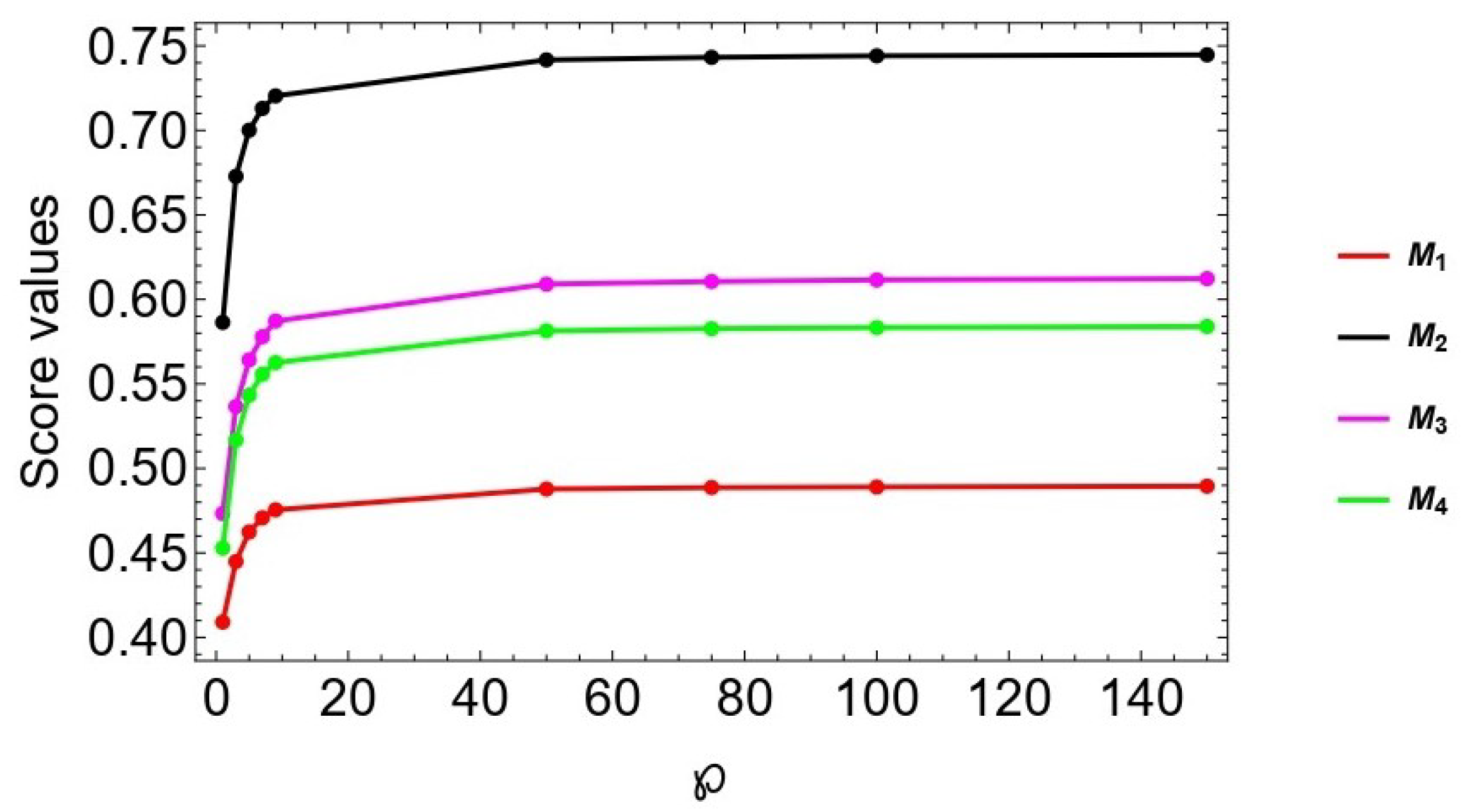
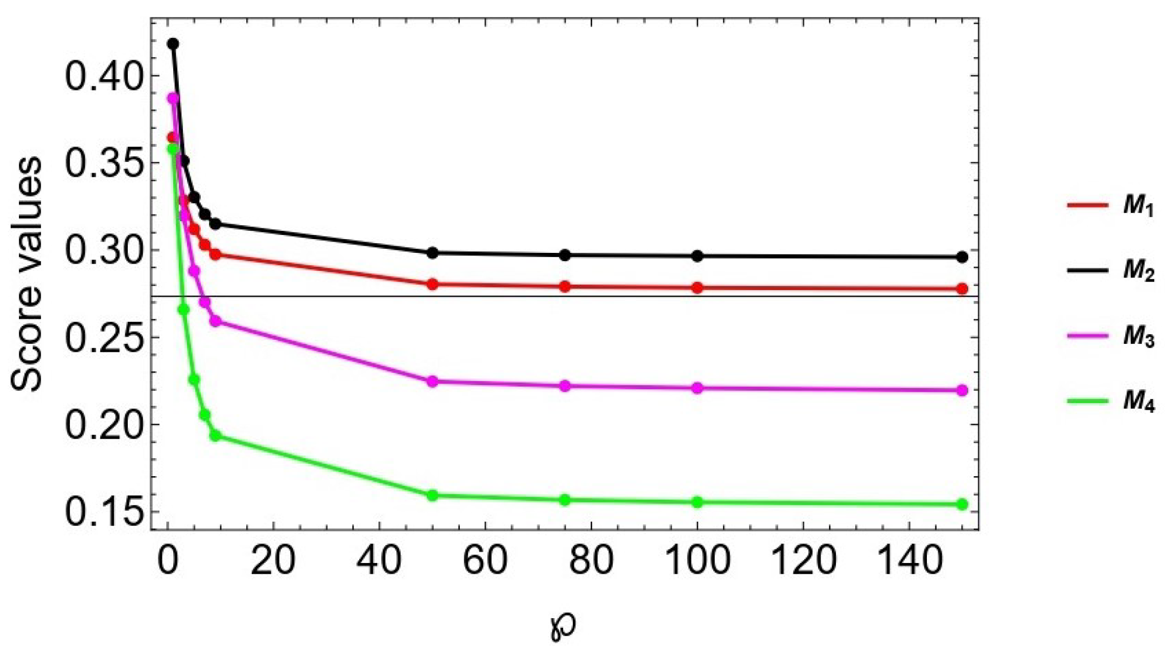
To examine the impacts of parameter in our proposed technique, a test was carried out using our case study with various values of this parameter; for = ( 1 , 3 , 5 , 7 , 9 , 50 , 75 , 100 , 150 ) . The influence of this parameter on ranking orders is depicted in Figure 4 and Figure 5. The score values of model M i ( i = 1 , 2 , , m ) based on the Ct-SFAAHA and Ct-SFAAHG operators are shown in Table 3 and Table 4, respectively. It is clear that as the value of for the Ct-SFAAHA operator increases, so do the score values of the accessible alternatives; however, when the magnitude of for the Ct-SFAAHG operator grows, the score values of the alternatives decrease. In both scenarios, the associated ranking results remain the same, indicating that the framed approach always has the isotonicity property, allowing DEs to select the optimal value according to their preferences. Based on these values and analysis, it is concluded that a DE may select the appropriate value of based on its decision-making behavior. For instance, if the DE is the most hopeful about the choice, he or she might select the Ct-SFAAHG operator with lower values. If, on the other hand, he/she selects the Ct-SFAAHA operator to aggregate the process, he/she may use bigger values for the parameters . Furthermore, if a DE deploys the Ct-SFAAHA operator throughout the aggregation process to obtain the most pessimistic choice, he or she might choose lower values of . The impact of values on decision-making increases the adaptability of our suggested technique since DEs are able to modify the parameters based on their preferences and actual scenarios. Furthermore, as seen in Figure 4 and Figure 5, even though the values of vary during the example, the outputs of the options seem to be the same, confirming the consistency of the provided operators.

7. Comparative Analysis

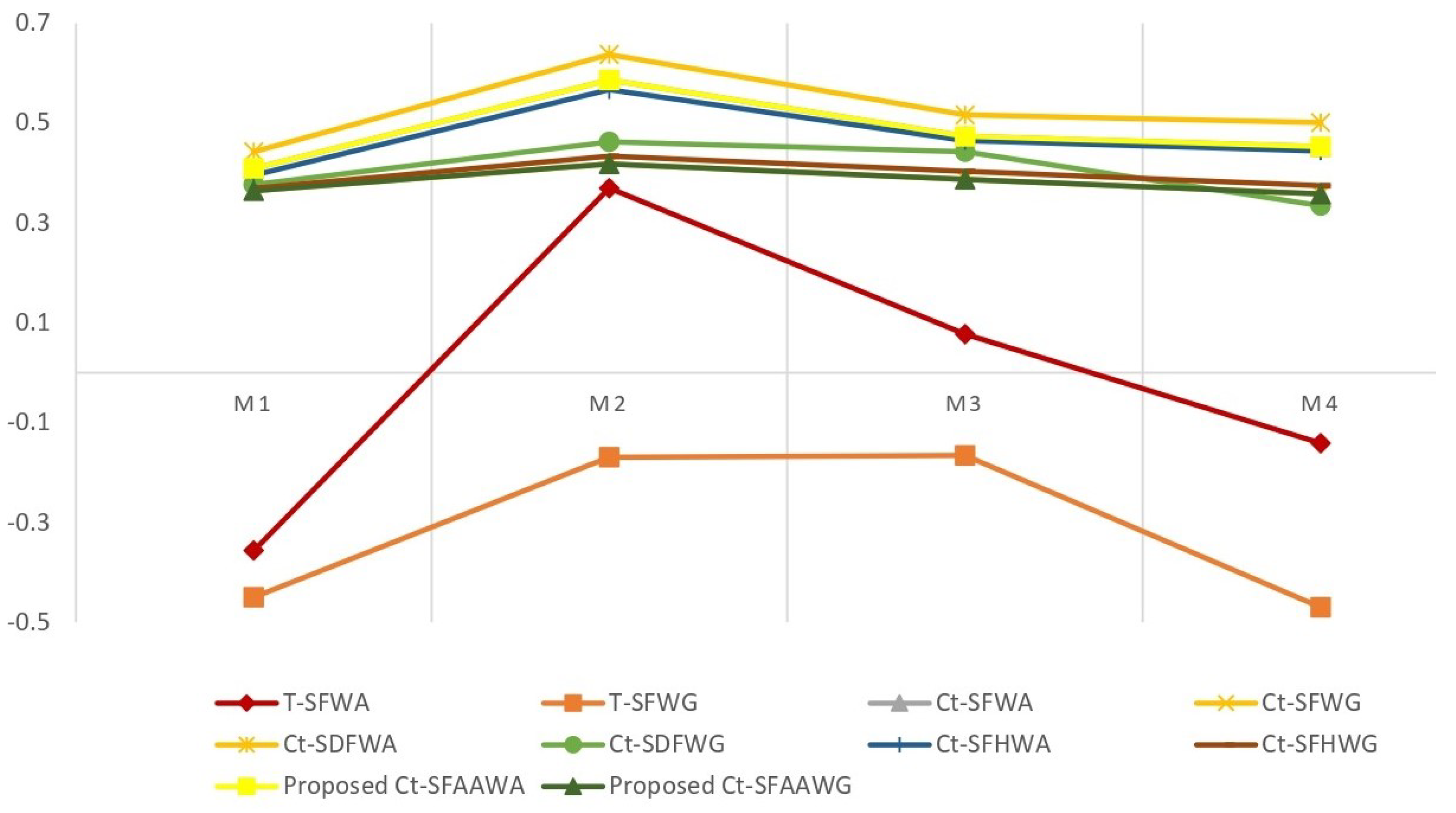
In this section, a comparative study with numerous existing spherical fuzzy decision approaches is implemented to demonstrate the efficacy and practicability of the proposed methodology. Our suggested ranking methodology is compared with existing operators, such as the t-spherical fuzzy weighted averaging (T-SFWA) operator [22], t-spherical fuzzy weighted geometric (T-SFWG) operator [22], complex t-spherical fuzzy weighted averaging (Ct-SFWA) operator [39], complex t-spherical fuzzy weighted geometric (Ct-SFWG) operator [39], complex t-spherical Dombi fuzzy weighted averaging (Ct-SDFWA) operator [42], complex t-spherical Dombi fuzzy weighted geometric (Ct-SDFWG) operator [42], complex t-spherical fuzzy Hamacher weighted averaging (Ct-SFHWA) operator [57], complex t-spherical fuzzy Hamacher weighted geometric (Ct-SFHWG) operator [57], and the technique for order of preference by similarity to the ideal solution (TOPSIS) [58] and TOPSIS [59]. To ensure the rationality of the comparison process, we used the weight vector determined in this research to solve the above vehicle model problem based on the listed methods. The ranks of models derived from the aforementioned methodologies are outlined in Table 5.
1. 
We compare our approach with the T-SFWA and T-SFWG operators suggested by Mahmood et al. [22], by taking parameter t = 3. The ranking result was derived by utilizing T-SFWG operators is M 3 M 2 M 4 M 1 . We have M 3 as the best model albeit M 3 is ranked as the second best model accordingly to our proposed and other existing models. This difference in the outcome is justified since the suggested technique assessed the alternatives by taking amplitude and phase factors into account simultaneously, while T-SFWA and T-SFWG took amplitude terms into account only during the aggregation step. It led to a loss of information regarding the duration of the influence of model M i ( i = 1 , 2 , 3 , 4 ) , since the phase terms in our studied problem represent the time span of the influence, as mentioned in Section 2. This debate leads to the conclusion that in time-periodic issues, ignoring the phase terms that offer information about periodicity and using the existing aggregation operators [22] in the t-spherical fuzzy environment do not provide practical answers. As a result, techniques in the t-spherical fuzzy environment are incapable of dealing with time-periodic and two-dimensional situations. The suggested technique, on the other hand, may be used to tackle MCDM issues in complex fuzzy settings. As a result, the methodology described here is more generic and successful in dealing with MCDM challenges.
2. 
From the listed results in Table 5 and Figure 6, it is clear that the ranking outcomes acquired by the Ct-SFWA and Ct-SFWG operators [39] based on algebraic operations totally match the proposed aggregation operators’ results. This similarity in the results is justifiable because Ct-SFWA and Ct-SFWG operators [39] are special instances of our initiated operators Ct-SFAAWA and Ct-SFAAWG, respectively, and these would be the cases for = 1 . The presented operators have the major benefit of having a flexible parameter that allows the DE to make judgments by altering its value. It is also seen that the existing operators [39] use score and accuracy functions, which have many weak aspects (see [42]). It is worth noting that for rational comparison, in the present study, we calculated the score values of the aggregated results supplied by Ct-SFWA and Ct-SFWG operators using the revised score function [42] since it works well and accurately distributes objects when the existing score function fails to do so.
3. 
Employing Ct-SDFWA and Ct-SDFWG [42] operators, the ranking outcomes are acquired as M 2 M 3 M 4 M 1 , which is the same as derived by our initiated Ct-SFAAWA operator. The existing operators [42] are based on the Dombi t-norm and t-conorm, and do not follow the property of isotonicity as can be seen from Tables 18 and 19 of Reference [42]. On the other hand, the proposed Ct-SFAAWA (Ct-SFAAWG) operator values grow (reduce) monotonically with the increase of parameter , allowing DEs to select the right value based on their risk preferences. If the DEs are risk preference, they may take the parameter value as low as fairly practicable; if the DEs are risk aversion, they can take the parameter value as high as reasonably achievable in the case of the Ct-SFAAWA operator, and vice versa for the Ct-SFAAWG operator. Thus, the DEs can use the appropriate parameter value based on their risk tolerance and real demands.
4. 
It can be noticed from Table 5 that the sorting outcomes of vehicle models through employing Zedam et al.’s [57] approach are basically the same as the proposed one. However, Zedam et al.’s approach, including the other previous approaches [22,39,42], presume that DEs would assign weights to criteria based on their subjective experiences, knowledge background, and cognitive capacities, which often place too much dependence on professional expertise and lead to illogical conclusions. In contrast, the suggested technique considers objective weight indicated by entropy, which increases the proposed strategy’s practicality in dealing with challenging situations. Furthermore, the work presented by [58,59] is a limited notion and can work only with complex spherical fuzzy data, i.e., 0 μ ( ) 2 + ϑ ( ) 2 + ν ( ) 2 1 , 0 ð μ 2 + ð ϑ 2 + ð ν 2 1 . From this restriction, it is clear that [58,59] approaches are not capable of handling the data given in Table 1. From Table 1, it is easy to see that μ 22 , ϑ 22 , ν 22 = 0.8 , 0.2 , 0.6 is not complex spherical fuzzy data because 0.8 2 + 0.2 2 + 0.6 2 1 . Due to this, the data provided in Table 1 cannot be handled by [58,59].
Aside from the comparisons mentioned above, we also compare certain essential properties of our proposed MCDM with the existing approaches. The symbol “✔” in the Table 6 indicates that the technique meets those requirements; the symbol “×” indicates that the related procedure fails.
Table 5. Ranking results based on different aggregation operators.
Operator S M 1 S M 2 S M 3 S M 4 Ranking
T-SFWA [22]−0.35650.36980.0774−0.1416 M 2 M 3 M 4 M 1
T-SFWG [22]−0.4502−0.1697−0.1659−0.4699 M 3 M 2 M 4 M 1
Ct-SFWA [39]0.40910.58640.47340.4529 M 2 M 3 M 4 M 1
Ct-SFWG [39]0.36450.41810.38700.3580 M 2 M 3 M 1 M 4
Ct-SDFWA [42]0.44260.63740.51680.5011 M 2 M 3 M 4 M 1
Ct-SDFWG [42]0.37720.46230.44290.3346 M 2 M 3 M 4 M 1
Ct-SFHWA [57]0.39570.56690.46450.4438 M 2 M 3 M 4 M 1
Ct-SFHWG [57]0.36940.43380.40370.3746 M 2 M 3 M 4 M 1
TOPSIS [58]Failed
TOPSIS [59]Failed
Proposed Ct-SFAAWA0.40910.58640.47330.4529 M 2 M 3 M 4 M 1
Proposed Ct-SFAAWG0.36450.41820.38700.3580 M 2 M 3 M 1 M 4
Table 6. Comparison of the proposed model with extant models in the literature.
ModelPeriodicityDetermination of Criteria WeightsHandles Optimistic as Well Pessimistic BehaviorBroader Uncertain SpaceExtra ParameterProperty of IsotonicityRepresents Two Dimensional Information
[22]××××××
[39]××××
[42]×××
[57]×××
[58]××××
[59]××××
Proposed
Figure 6. Comparative analysis with existing aggregation operators.
Symmetry 15 00085 g006

8. Conclusions and Future Work Plan

The core contributions of the study are summarized as follows:
(i)
In this study, we introduced the decision-making method based on AA aggregation operators to tackle the MCDM problems with unknown weight information. However, the uncertainties that exist in the data collection are managed with the aid of the Ct-SFS features. In the present work, we took the AA-weighted average and geometric operator to aggregate the different preferences of the alternatives. The main benefit of the considered AA operators is that they generalize the theories to more extended manners. Furthermore, the flexible parameters in the study help the DE to pick it depending on his/her own preferences. Moreover, the considered research equivalently manages the uncertainty with the change to the phase (periodicity) of the data.
(ii)
The aggregation operators, i.e., Ct-SFAAWA, Ct-SFAAOWA, Ct-SFAAHA, Ct-SFAAWG, Ct-SFAAOWG, and Ct-SFAAHG, are devised based on the proposed AA t-norm and t-conorm operational laws. These stated operators aggregate the different preferences of the DE into the collective number. Moreover, we studied that several of the existing studies are considered special cases. Furthermore, various desirable properties and peculiar instances are elaborated upon. In addition, the complex t-spherical fuzzy entropy measure is advanced to ascertain the weights of criteria. Following this, an innovative complex t-spherical fuzzy MCDM method is presented based on initiated operators and entropy measures to settle complex decision problems; this model can overcome the defects of the extant methods that only consider the weight information to be known.
(iii)
A practical problem about vehicle model selection is addressed to demonstrate the efficacy and viability of our proposed method. In addition, the parameter analysis and a comparison between our suggested technique and earlier spherical fuzzy decision methods were done to demonstrate the validity and outstanding advantages of the developed MCDM method. The results demonstrate that the proposed approach has a certain degree of accessibility and distinctive benefits.
However, the presented approach also has certain limitations: (a) it disregards the weight information of DEs; (b) it fails to take into account the consistency of DEs during expert information fusion; and (c) it presupposes that the DEs in the decision procedure are totally rational.
In light of the deficiencies in the provided scheme, future research on uncertain decision methods and applications will focus on the following aspects: (1) proposing several novel complex t-spherical fuzzy AA operators by combining power average operators, Muirhead mean, and partitioned hamy mean operators; (2) exploring and discussing the novel information measures, such as dissimilar measures, knowledge measures, and divergence measures to support complex t-spherical fuzzy decision analyses; and (3) using the proposed MCDM approach to address other realistic decision methods, such as a sustainable supply chain [60], enterprise resource planning [61], solid waste management [62], and an emergency scheme assessment [63]; (4) constructing a large-scale group-decision-making model based on consensus reaching [64].

Author Contributions

Conceptualization, J.A. and M.N.; methodology, J.A.; software, M.N.; validation, J.A.; formal analysis, J.A.; investigation, M.N.; resources, J.A.; data curation, M.N.; writing—original draft preparation, J.A.; writing—review and editing, J.A.; visualization, J.A.; supervision, M.N.; project administration, M.N.; funding acquisition, M.N. All authors have read and agreed to the published version of the manuscript.

Funding

The authors would like to thank the Deanship of Scientific Research at Umm Al-Qura University for supporting this work by Grant Code:(22UQU4310396DSR46).

Data Availability Statement

All data generated or analyzed during this study are included in this published article.

Acknowledgments

The authors thank the editor and the anonymous referees for their constructive comments and suggestions.

Conflicts of Interest

The authors declare no conflict of interest.

References

  1. Ali, J. Hesitant fuzzy partitioned Maclaurin symmetric mean aggregation operators in multi-criteria decision-making. Phys. Scr. 2022, 97, 075208. [Google Scholar] [CrossRef]
  2. Ali, J. A novel score function based CRITIC-MARCOS method with spherical fuzzy information. Comput. Appl. Math. 2021, 40, 280. [Google Scholar] [CrossRef]
  3. Ali, J.; Bashir, Z.; Rashid, T. On distance measure and TOPSIS model for probabilistic interval-valued hesitant fuzzy sets: Application to healthcare facilities in public hospitals. Grey Syst. Theory Appl. 2022, 12, 197–229. [Google Scholar] [CrossRef]
  4. Bashir, Z.; Ali, J.; Rashid, T. Consensus-based robust decision making methods under a novel study of probabilistic uncertain linguistic information and their application in Forex investment. Artif. Intell. Rev. 2021, 54, 2091–2132. [Google Scholar] [CrossRef]
  5. Ali, J.; Bashir, Z.; Rashid, T. WASPAS-based decision making methodology with unknown weight information under uncertain evaluations. Expert Syst. Appl. 2021, 168, 114143. [Google Scholar] [CrossRef]
  6. Zadeh, L.A. Fuzzy sets. Inf. Control 1965, 8, 338–353. [Google Scholar] [CrossRef] [Green Version]
  7. Yuan, K.; Xu, W.; Li, W.; Ding, W. An incremental learning mechanism for object classification based on progressive fuzzy three-way concept. Inf. Sci. 2022, 584, 127–147. [Google Scholar] [CrossRef]
  8. Ali, J.; Bashir, Z.; Rashid, T. Weighted interval-valued dual-hesitant fuzzy sets and its application in teaching quality assessment. Soft Comput. 2021, 25, 3503–3530. [Google Scholar] [CrossRef]
  9. Ayaz, T.; Al-Shomrani, M.M.; Abdullah, S.; Hussain, A. Evaluation of enterprise production based on spherical cubic Hamacher aggregation operators. Mathematics 2020, 8, 1761. [Google Scholar] [CrossRef]
  10. Bashir, Z.; Bashir, Y.; Rashid, T.; Ali, J.; Gao, W. A novel multi-attribute group decision-making approach in the framework of proportional dual hesitant fuzzy sets. Appl. Sci. 2019, 9, 1232. [Google Scholar] [CrossRef]
  11. Malik, M.; Bashir, Z.; Rashid, T.; Ali, J. Probabilistic hesitant intuitionistic linguistic term sets in multi-attribute group decision making. Symmetry 2018, 10, 392. [Google Scholar] [CrossRef] [Green Version]
  12. Saha, A.; Dutta, D.; Kar, S. Some new hybrid hesitant fuzzy weighted aggregation operators based on Archimedean and Dombi operations for multi-attribute decision making. Neural Comput. Appl. 2021, 33, 8753–8776. [Google Scholar] [CrossRef]
  13. Alaoui, M.K.; Alharbi, F.; Zaland, S. Novel Analysis of Fuzzy Physical Models by Generalized Fractional Fuzzy Operators. J. Funct. Spaces 2022, 2022, 2504031. [Google Scholar] [CrossRef]
  14. Atanassov, K. Intuitionistic fuzzy sets. Fuzzy Sets Syst. 1986, 20, 87–96. [Google Scholar] [CrossRef]
  15. Yager, R.R. Pythagorean fuzzy subsets. In Proceedings of the 2013 Joint IFSA World Congress and NAFIPS Annual Meeting (IFSA/NAFIPS), Edmonton, AB, Canada, 24–28 June 2013; pp. 57–61. [Google Scholar]
  16. Yager, R.R. Generalized orthopair fuzzy sets. IEEE Trans. Fuzzy Syst. 2016, 25, 1222–1230. [Google Scholar] [CrossRef]
  17. Wei, G.; Gao, H.; Wei, Y. Some q-rung orthopair fuzzy Heronian mean operators in multiple attribute decision making. Int. J. Intell. Syst. 2018, 33, 1426–1458. [Google Scholar] [CrossRef]
  18. Shu, X.; Ai, Z.; Xu, Z.; Ye, J. Integrations of q-rung orthopair fuzzy continuous information. IEEE Trans. Fuzzy Syst. 2019, 27, 1974–1985. [Google Scholar] [CrossRef]
  19. Khan, M.J.; Ali, M.I.; Kumam, P. A new ranking technique for q-rung orthopair fuzzy values. Int. J. Intell. Syst. 2021, 36, 558–592. [Google Scholar] [CrossRef]
  20. Ali, J.; Bashir, Z.; Rashid, T.; Mashwani, W.K. A q-rung orthopair hesitant fuzzy stochastic method based on regret theory with unknown weight information. J. Ambient. Intell. Humaniz. Comput. 2022, 1–18. [Google Scholar] [CrossRef]
  21. Cuong, B.C.; Kreinovich, V. Picture fuzzy sets. J. Comput. Sci. Cybern. 2014, 30, 409–420. [Google Scholar]
  22. Mahmood, T.; Ullah, K.; Khan, Q.; Jan, N. An approach toward decision-making and medical diagnosis problems using the concept of spherical fuzzy sets. Neural Comput. Appl. 2019, 31, 7041–7053. [Google Scholar] [CrossRef]
  23. Kutlu Gündoğdu, F.; Kahraman, C. Spherical fuzzy sets and spherical fuzzy TOPSIS method. J. Intell. Fuzzy Syst. 2019, 36, 337–352. [Google Scholar] [CrossRef]
  24. Kutlu Gundogdu, F.; Kahraman, C. Extension of WASPAS with spherical fuzzy sets. Informatica 2019, 30, 269–292. [Google Scholar] [CrossRef] [Green Version]
  25. Kutlu Gündoğdu, F.; Kahraman, C. A novel spherical fuzzy analytic hierarchy process and its renewable energy application. Soft Comput. 2020, 24, 4607–4621. [Google Scholar] [CrossRef]
  26. Ullah, K.; Garg, H.; Gul, Z.; Mahmood, T.; Khan, Q.; Ali, Z. Interval valued T-spherical fuzzy information aggregation based on Dombi t-norm and Dombi t-conorm for multi-attribute decision making problems. Symmetry 2021, 13, 1053. [Google Scholar] [CrossRef]
  27. Guleria, A.; Bajaj, R.K. T-spherical fuzzy graphs: Operations and applications in various selection processes. Arab. J. Sci. Eng. 2020, 45, 2177–2193. [Google Scholar] [CrossRef]
  28. Mahnaz, S.; Ali, J.; Malik, M.A.; Bashir, Z. T-spherical fuzzy Frank aggregation operators and their application to decision making with unknown weight information. IEEE Access 2021, 10, 7408–7438. [Google Scholar] [CrossRef]
  29. Akram, M.; Alsulami, S.; Khan, A.; Karaaslan, F. Multi-criteria group decision-making using spherical fuzzy prioritized weighted aggregation operators. Int. J. Comput. Intell. Syst. 2020, 13, 1429–1446. [Google Scholar] [CrossRef]
  30. Yang, W.; Pang, Y. T-Spherical Fuzzy Bonferroni Mean Operators and Their Application in Multiple Attribute Decision Making. Mathematics 2022, 10, 988. [Google Scholar] [CrossRef]
  31. Ramot, D.; Milo, R.; Friedman, M.; Kandel, A. Complex fuzzy sets. IEEE Trans. Fuzzy Syst. 2002, 10, 171–186. [Google Scholar] [CrossRef]
  32. Ramot, D.; Friedman, M.; Langholz, G.; Kandel, A. Complex fuzzy logic. IEEE Trans. Fuzzy Syst. 2003, 11, 450–461. [Google Scholar] [CrossRef]
  33. Alkouri, A.M.J.S.; Salleh, A.R. Complex intuitionistic fuzzy sets. In Proceedings of the AIP Conference Proceedings; American Institute of Physics: New York, NY, USA, 2012; Volume 1482, pp. 464–470. [Google Scholar]
  34. Rani, D.; Garg, H. Distance measures between the complex intuitionistic fuzzy sets and their applications to the decision-making process. Int. J. Uncertain. Quantif. 2017, 7, 423–439. [Google Scholar] [CrossRef]
  35. Rani, D.; Garg, H. Complex intuitionistic fuzzy power aggregation operators and their applications in multicriteria decision-making. Expert Syst. 2018, 35, e12325. [Google Scholar] [CrossRef]
  36. Garg, H.; Rani, D. Some generalized complex intuitionistic fuzzy aggregation operators and their application to multicriteria decision-making process. Arab. J. Sci. Eng. 2019, 44, 2679–2698. [Google Scholar] [CrossRef]
  37. Garg, H.; Rani, D. Generalized geometric aggregation operators based on t-norm operations for complex intuitionistic fuzzy sets and their application to decision-making. Cogn. Comput. 2020, 12, 679–698. [Google Scholar] [CrossRef]
  38. Ullah, K.; Mahmood, T.; Ali, Z.; Jan, N. On some distance measures of complex Pythagorean fuzzy sets and their applications in pattern recognition. Complex Intell. Syst. 2020, 6, 15–27. [Google Scholar] [CrossRef] [Green Version]
  39. Ali, Z.; Mahmood, T.; Yang, M.S. Complex T-spherical fuzzy aggregation operators with application to multi-attribute decision making. Symmetry 2020, 12, 1311. [Google Scholar] [CrossRef]
  40. Akram, M.; Kahraman, C.; Zahid, K. Group decision-making based on complex spherical fuzzy VIKOR approach. Knowl.-Based Syst. 2021, 216, 106793. [Google Scholar] [CrossRef]
  41. Nasir, A.; Jan, N.; Yang, M.S.; Khan, S.U. Complex T-spherical fuzzy relations with their applications in economic relationships and international trades. IEEE Access 2021, 9, 66115–66131. [Google Scholar] [CrossRef]
  42. Karaaslan, F.; Dawood, M.A.D. Complex T-spherical fuzzy Dombi aggregation operators and their applications in multiple-criteria decision-making. Complex Intell. Syst. 2021, 7, 2711–2734. [Google Scholar] [CrossRef]
  43. Khan, R.; Ullah, K.; Pamucar, D.; Bari, M. Performance measure using a multi-attribute decision making approach based on Complex T-spherical fuzzy power aggregation operators. J. Comput. Cogn. Eng. 2022, 1, 138–146. [Google Scholar] [CrossRef]
  44. Aczél, J.; Alsina, C. Characterizations of some classes of quasilinear functions with applications to triangular norms and to synthesizing judgements. Aequationes Math. 1982, 25, 313–315. [Google Scholar] [CrossRef]
  45. Wang, N.; Li, Q.; Abd El-Latif, A.A.; Yan, X.; Niu, X. A novel hybrid multibiometrics based on the fusion of dual iris, visible and thermal face images. In Proceedings of the 2013 International Symposium on Biometrics and Security Technologies, Chengdu, China, 2–5 July 2013; pp. 217–223. [Google Scholar]
  46. Senapati, T.; Chen, G.; Yager, R.R. Aczel-Alsina aggregation operators and their application to intuitionistic fuzzy multiple attribute decision making. Int. J. Intell. Syst. 2022, 37, 1529–1551. [Google Scholar] [CrossRef]
  47. Senapati, T.; Chen, G.; Mesiar, R.; Yager, R.R. Novel Aczel–Alsina operations-based interval-valued intuitionistic fuzzy aggregation operators and their applications in multiple attribute decision-making process. Int. J. Intell. Syst. 2022, 37, 5059–5081. [Google Scholar] [CrossRef]
  48. Senapati, T. Approaches to multi-attribute decision-making based on picture fuzzy Aczel–Alsina average aggregation operators. Comput. Appl. Math. 2022, 41, 1–19. [Google Scholar] [CrossRef]
  49. Naeem, M.; Ali, J. A novel multi-criteria group decision-making method based on Aczel–Alsina spherical fuzzy aggregation operators: Application to evaluation of solar energy cells. Phys. Scr. 2022, 97, 085203. [Google Scholar] [CrossRef]
  50. Ali, J.; Naeem, M. Complex q-Rung Orthopair Fuzzy Aczel–Alsina aggregation operators and its application to multiple criteria decision-making with unknown weight information. IEEE Access 2022, 10, 85315–85342. [Google Scholar] [CrossRef]
  51. Hussain, A.; Ullah, K.; Yang, M.S.; Pamucar, D. Aczel-Alsina Aggregation Operators on T-Spherical Fuzzy (TSF) Information with Application to TSF Multi-Attribute Decision Making. IEEE Access 2022, 10, 26011–26023. [Google Scholar] [CrossRef]
  52. Mahmood, T.; ur Rehman, U.; Ali, Z. Analysis and Application of Aczel-Alsina Aggregation operators Based on Bipolar Complex Fuzzy Information in Multiple Attribute Decision Making. Inf. Sci. 2022, 619, 817–833. [Google Scholar] [CrossRef]
  53. Menger, K. Statistical metrics. Proc. Natl. Acad. Sci. USA 1942, 28, 535. [Google Scholar] [CrossRef] [Green Version]
  54. Klement, E.P.; Mesiar, R.; Pap, E. Triangular Norms; Springer Science & Business Media: Dordrecht, The Netherlands, 2013; Volume 8. [Google Scholar]
  55. Alsina, C.; Schweizer, B.; Frank, M.J. Associative Functions: Triangular Norms and Copulas; World Scientific: Singapore, 2006. [Google Scholar]
  56. Garg, H.; Rani, D. New prioritized aggregation operators with priority degrees among priority orders for complex intuitionistic fuzzy information. J. Ambient. Intell. Humaniz. Comput. 2021, 1–27. [Google Scholar] [CrossRef]
  57. Zedam, L.; Pehlivan, N.Y.; Ali, Z.; Mahmood, T. Novel Hamacher Aggregation Operators Based on Complex T-Spherical Fuzzy Numbers for Cleaner Production Evaluation in Gold Mines. Int. J. Fuzzy Syst. 2022, 24, 2333–2353. [Google Scholar] [CrossRef]
  58. Ali, Z.; Mahmood, T.; Yang, M.S. TOPSIS method based on complex spherical fuzzy sets with Bonferroni mean operators. Mathematics 2020, 8, 1739. [Google Scholar] [CrossRef]
  59. Akram, M.; Kahraman, C.; Zahid, K. Extension of TOPSIS model to the decision-making under complex spherical fuzzy information. Soft Comput. 2021, 25, 10771–10795. [Google Scholar] [CrossRef]
  60. He, L.; Wu, Z.; Xiang, W.; Goh, M.; Xu, Z.; Song, W.; Ming, X.; Wu, X. A novel Kano-QFD-DEMATEL approach to optimise the risk resilience solution for sustainable supply chain. Int. J. Prod. Res. 2021, 59, 1714–1735. [Google Scholar] [CrossRef]
  61. Ullah, K. Picture fuzzy Maclaurin symmetric mean operators and their applications in solving multiattribute decision-making problems. Math. Probl. Eng. 2021, 2021, 1098631. [Google Scholar] [CrossRef]
  62. Garg, H.; Rani, D. An efficient intuitionistic fuzzy MULTIMOORA approach based on novel aggregation operators for the assessment of solid waste management techniques. Appl. Intell. 2022, 52, 4330–4363. [Google Scholar] [CrossRef]
  63. Huang, L.; Mao, L.X.; Chen, Y.; Liu, H.C. New method for emergency decision making with an integrated regret theory-EDAS method in 2-tuple spherical linguistic environment. Appl. Intell. 2022, 52, 13296–13309. [Google Scholar] [CrossRef]
  64. Wan, S.P.; Yan, J.; Dong, J.Y. Personalized individual semantics based consensus reaching process for large-scale group decision making with probabilistic linguistic preference relations and application to COVID-19 surveillance. Expert Syst. Appl. 2022, 191, 116328. [Google Scholar] [CrossRef]
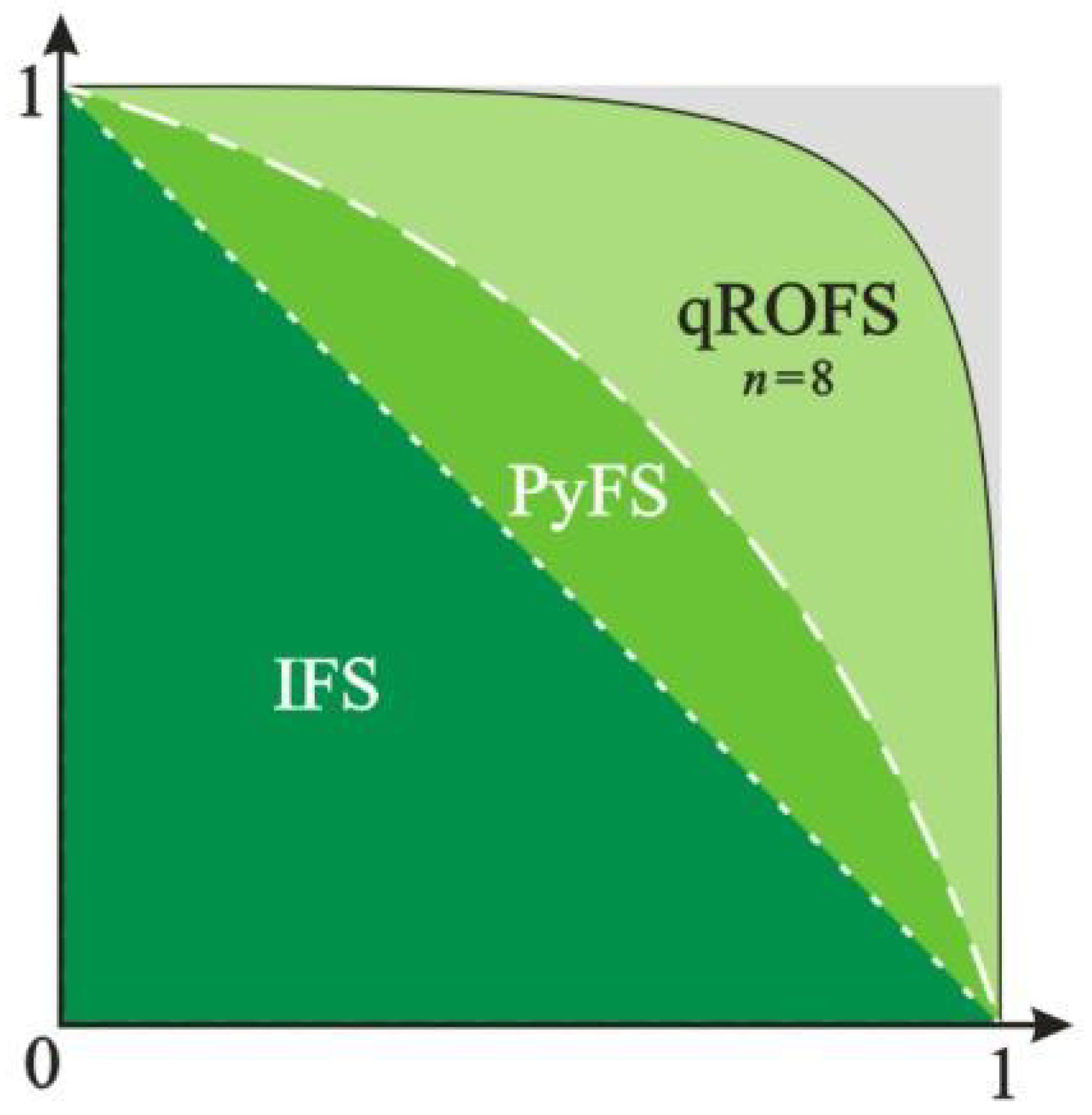
Figure 1. Evaluation of ranges of IFS, PyFS, and qROFS.
Symmetry 15 00085 g001
Figure 2. Evaluation of ranges of PFS, SFS, and t-SFS.
Symmetry 15 00085 g002
Figure 3. Flowchart of the presented method.
Symmetry 15 00085 g003
Figure 4. Ranking of alternatives for different values by the Ct-ROFAAWA operator.
Symmetry 15 00085 g004
Figure 5. Ranking of alternatives for different values by the Ct-ROFAAWG operator.
Symmetry 15 00085 g005
Table 1. Complex t-spherical fuzzy decision matrix C.
κ 1 κ 2 κ 3 κ 4
a l t 1 0.7 e i 2 π ( 5 12 ) , 0.2 e i 2 π ( 4 12 ) , 0.1 e i 2 π ( 2 12 ) 0.3 e i 2 π ( 4 12 ) , 0.4 e i 2 π ( 6 12 ) , 0.5 e i 2 π ( 2 12 ) 0.1 e i 2 π ( 5 12 ) , 0.4 e i 2 π ( 5 12 ) , 0.8 e i 2 π ( 7 12 ) 0.5 e i 2 π ( 5 12 ) , 0.3 e i 2 π ( 1 12 ) , 0.3 e i 2 π ( 3 12 )
a l t 2 0.4 e i 2 π ( 5 12 ) , 0.7 e i 2 π ( 7 12 ) , 0.2 e i 2 π ( 1 12 ) 0.8 e i 2 π ( 8 12 ) , 0.2 e i 2 π ( 1 12 ) , 0.6 e i 2 π ( 2 12 ) 0.9 e i 2 π ( 3 12 ) , 0.5 e i 2 π ( 7 12 ) , 0.3 e i 2 π ( 5 12 ) 0.3 e i 2 π ( 4 12 ) , 0.3 e i 2 π ( 2 12 ) , 0.2 e i 2 π ( 3 12 )
a l t 3 0.1 e i 2 π ( 2 12 ) , 0.6 e i 2 π ( 10 12 ) , 0.3 e i 2 π ( 4 12 ) 0.7 e i 2 π ( 6 12 ) , 0.2 e i 2 π ( 5 12 ) , 0.3 e i 2 π ( 4 12 ) 0.6 e i 2 π ( 7 12 ) , 0.5 e i 2 π ( 8 12 ) , 0.6 e i 2 π ( 3 12 ) 0.4 e i 2 π ( 2 12 ) , 0.7 e i 2 π ( 9 12 ) , 0.4 e i 2 π ( 3 12 )
a l t 4 0.9 e i 2 π ( 8 12 ) , 0.4 e i 2 π ( 3 12 ) , 0.4 e i 2 π ( 5 12 ) 0.7 e i 2 π ( 2 12 ) , 0.5 e i 2 π ( 4 12 ) , 0.3 e i 2 π ( 5 12 ) 0.4 e i 2 π ( 5 12 ) , 0.3 e i 2 π ( 3 12 ) , 0.6 e i 2 π ( 6 12 ) 0.5 e i 2 π ( 2 12 ) , 0.7 e i 2 π ( 3 12 ) , 0.2 e i 2 π ( 4 12 )
Table 2. Normalized complex t-spherical fuzzy decision matrix N.
κ 1 κ 2 κ 3 κ 4
a l t 1 0.1 e i 2 π ( 2 12 ) , 0.2 e i 2 π ( 4 12 ) , 0.7 e i 2 π ( 5 12 ) 0.3 e i 2 π ( 4 12 ) , 0.4 e i 2 π ( 6 12 ) , 0.5 e i 2 π ( 2 12 ) 0.1 e i 2 π ( 5 12 ) , 0.4 e i 2 π ( 5 12 ) , 0.8 e i 2 π ( 7 12 ) 0.3 e i 2 π ( 3 12 ) , 0.3 e i 2 π ( 1 12 ) , 0.5 e i 2 π ( 5 12 )
a l t 2 0.2 e i 2 π ( 1 12 ) , 0.7 e i 2 π ( 7 12 ) , 0.4 e i 2 π ( 5 12 ) 0.8 e i 2 π ( 8 12 ) , 0.2 e i 2 π ( 1 12 ) , 0.6 e i 2 π ( 2 12 ) 0.9 e i 2 π ( 3 12 ) , 0.5 e i 2 π ( 7 12 ) , 0.3 e i 2 π ( 5 12 ) 0.2 e i 2 π ( 3 12 ) , 0.3 e i 2 π ( 2 12 ) , 0.3 e i 2 π ( 4 12 )
a l t 3 0.3 e i 2 π ( 4 12 ) , 0.6 e i 2 π ( 10 12 ) , 0.1 e i 2 π ( 2 12 ) 0.7 e i 2 π ( 6 12 ) , 0.2 e i 2 π ( 5 12 ) , 0.3 e i 2 π ( 4 12 ) 0.6 e i 2 π ( 7 12 ) , 0.5 e i 2 π ( 8 12 ) , 0.6 e i 2 π ( 3 12 ) 0.4 e i 2 π ( 3 12 ) , 0.7 e i 2 π ( 9 12 ) , 0.4 e i 2 π ( 2 12 )
a l t 4 0.4 e i 2 π ( 5 12 ) , 0.4 e i 2 π ( 3 12 ) , 0.9 e i 2 π ( 8 12 ) 0.7 e i 2 π ( 2 12 ) , 0.5 e i 2 π ( 4 12 ) , 0.3 e i 2 π ( 5 12 ) 0.4 e i 2 π ( 5 12 ) , 0.3 e i 2 π ( 3 12 ) , 0.6 e i 2 π ( 6 12 ) 0.2 e i 2 π ( 4 12 ) , 0.7 e i 2 π ( 3 12 ) , 0.5 e i 2 π ( 2 12 )
Table 3. Ranking results by Ct-SFAAWA with various .
S M 1 S M 2 S M 3 S M 4 Ranking
= 1 0.40910.58640.47330.4529 M 2 M 3 M 4 M 1
= 3 0.44490.67280.53660.5168 M 2 M 3 M 4 M 1
= 5 0.46240.70010.56420.5433 M 2 M 3 M 4 M 1
= 7 0.47080.71300.57790.5557 M 2 M 3 M 4 M 1
= 9 0.47550.72040.58720.5626 M 2 M 3 M 4 M 1
= 50 0.48780.74170.60900.5814 M 2 M 3 M 4 M 1
= 75 0.48870.74320.61060.5827 M 2 M 3 M 4 M 1
= 100 0.48900.74410.61150.5833 M 2 M 3 M 4 M 1
= 150 0.48950.74470.61230.5840 M 2 M 3 M 4 M 1
Table 4. Ranking results by Ct-SFAAWG with various .
S M 1 S M 2 S M 3 S M 4 Ranking
= 1 0.36450.41820.38700.3580 M 2 M 3 M 1 M 4
= 3 0.32850.35110.31960.2659 M 2 M 3 M 1 M 4
= 5 0.31200.33030.28800.2258 M 2 M 3 M 1 M 4
= 7 0.30300.32050.27030.2056 M 2 M 3 M 1 M 4
= 9 0.29750.31500.25930.1937 M 2 M 3 M 1 M 4
= 50 0.28040.29840.22470.1594 M 2 M 3 M 1 M 4
= 75 0.27910.29710.22210.1568 M 2 M 3 M 1 M 4
= 100 0.27840.29660.22090.1555 M 2 M 3 M 1 M 4
= 150 0.27780.29600.21960.1543 M 2 M 3 M 1 M 4
Disclaimer/Publisher’s Note: The statements, opinions and data contained in all publications are solely those of the individual author(s) and contributor(s) and not of MDPI and/or the editor(s). MDPI and/or the editor(s) disclaim responsibility for any injury to people or property resulting from any ideas, methods, instructions or products referred to in the content.