Protectability of IBMQ Qubits by Dynamical Decoupling Technique

Abstract

We study the current effectiveness of the dynamical decoupling technique on a publicly accessible IBM quantum computer (IBMQ). This technique, also known as bang-bang decoupling or dynamical symmetrization, consists of applying sequences of pulses for protecting a qubit from decoherence by symmetrizing the qubit–environment interactions. Works in the field have studied sequences with different symmetries and carried out tests on IBMQ devices typically considering single-qubit states. We show that the simplest universal sequences can be interesting for preserving two-qubit states on the IBMQ device. For this, we considered a collection of single-qubit and two-qubit states. The results indicate that a simple dynamical decoupling approach using available IBMQ pulses is not enough for protecting a general single-qubit state without further care. Nevertheless, the technique is beneficial for the Bell states. This encouraged us to study logical qubit encodings such as $\left\{{|0⟩}_L\equiv |01⟩,{|1⟩}_L\equiv |10⟩\right\}$, where a quantum state has the form $|{\psi }_{ab}⟩=a{|0⟩}_L+b{|1⟩}_L$. Thus, we explored the effectiveness of dynamical decoupling with a large set of two-qubit $|{\psi }_{ab}⟩$ states, where a and b are real amplitudes. With this, we also determined that the $|{\psi }_{ab}⟩$ states most benefiting from this dynamical decoupling approach and slowed down the decay of their survival probability.

1. Introduction

During the last few years, there has been a notable development of error correction for quantum computing [1,2,3]. However, due to the scheduling of the operations in quantum algorithms and protocols, it is usual to find time intervals when a qubit may remain inactive. During these wait periods, decoherence is an important factor to consider, as it causes the loss of the quantum information stored in the qubits. The interaction with the environment is the main driver of this phenomenon [1].

An interesting and simple way of mitigating the effects of the environmental noise is dynamical decoupling [4,5], also known as bang-bang decoupling or dynamical symmetrization. This is a quantum control technique that consists of applying tailored sequences of pulses to the considered quantum system in order to cancel (or average out) the interaction with the environment [4]. This is achieved by replacing the system–environment interaction Hamiltonian by a sequence of pulse-generated Hamiltonians, which are symmetrized so that their total average is canceled [6]. This can be beneficial for complex quantum information algorithms, as demonstrated in [7], and communication protocols, such as the one explained in [8] requiring wait times.

A large collection of dynamical decoupling pulse sequences has been studied [5,6,9,10]. These sequences differ from each other, for example in the type of electromagnetic pulses being used, the time intervals between pulses, and the pulse ordering. These characteristics allow creating a large catalog of sequences with different symmetries and performances. In the ideal theoretical case, this quantum control technique requires very short and strong pulses separated by the shortest time interval possible. There are sequences that only cancel out some components of the qubit–environment interaction Hamiltonian, and there are also sequences that cancel all the interaction components. The latter are known as universal decoupling sequences [5]. Some simple examples of universal sequences in the theoretical case are the XYXY, XZXZ, and YZYZ sequences, where X, Y, and Z represent the Pauli gates.

However, in reality, the pulses will have a given time duration and finite amplitude, which may leave uncorrected environment noise or introduce further errors [5]. Thus, the design of the adequate dynamical decoupling sequences is an important task, and symmetry considerations play a key role [5,11]. The idea of using sequences of frequent, short, and intense pulses is similar to the approach described by the quantum Zeno effect [12]. This highlights the importance of the pulse duration, as in the worst case scenario, it may induce “anti-Zeno-like” effects, doing further damage to the system.

Nevertheless, it can be very interesting to combine dynamical decoupling with logical qubit encodings in decoherence-free subspaces such as, for example, $\{{|0⟩}_L\equiv |01⟩,{|1⟩}_L\equiv |10⟩\}$ [5,13,14]. Logical qubit encodings are a known tool for fighting against noise errors, but physical superconducting qubits such as the ones from IBM are influenced by the effects of thermal relaxation [15], which can destroy the logical encoding. For example, the aforementioned ${|0⟩}_L\equiv |01⟩$ and ${|1⟩}_L\equiv |10⟩$ states naturally tend to relax to the physical ground state |00⟩. Therefore, dynamical decoupling can be useful for preserving the qubit encoding and to avoid thermal relaxation, dephasing, or qubit crosstalk errors [16]. This may improve the quality of quantum-error-correcting codes, where dynamical decoupling would be useful during the undesired wait times in the circuit gate layers to preserve information and to fight against undesired crosstalk or interactions with the environment [16,17].

In this work, we tested the current effectiveness of simple dynamical decoupling on a public IBM quantum computer experimentally. The sequences considered were the universal XYXY, XZXZ, and YZYZ sequences. We started by using dynamical decoupling in an attempt to protect the basic single-qubit states |0⟩ and |1⟩ from decoherence. We did the same with the four two-qubit Bell states. Following [18], these states are denoted as:

$$\begin{array}{cc}|{\beta }_{00}⟩={\displaystyle \frac{1}{\sqrt{2}}}\left(|00⟩+|11⟩\right),\hfill & |{\beta }_{01}⟩={\displaystyle \frac{1}{\sqrt{2}}}\left(|01⟩+|10⟩\right),\hfill \\ |{\beta }_{10}⟩={\displaystyle \frac{1}{\sqrt{2}}}\left(|00⟩-|11⟩\right),\hfill & |{\beta }_{11}⟩={\displaystyle \frac{1}{\sqrt{2}}}\left(|01⟩-|10⟩\right).\hfill \end{array}$$

(1)

Although the results indicate that this simple approach to the technique cannot fully protect an unknown state, we observed that dynamical decoupling is beneficial for Bell states: their survival probability decay can be slowed down within the times considered. $|{\beta }_{01}⟩$ and $|{\beta }_{11}⟩$ are included in the set of states with the form $|{\psi }_{ab}⟩=a|01⟩+b|10⟩$, where a and b are real values. Thus, we performed further tests by considering the set of states $|{\psi }_{ab}⟩$, which also included the aforementioned ${|0⟩}_L\equiv |01⟩$ and ${|1⟩}_L\equiv |10⟩$ states. With this, we indicate the $|{\psi }_{ab}⟩$ states most benefiting from dynamical decoupling in the IBM five-qubit quantum computer.

2. Materials and Methods

To carry out the experiments, we employed the ibmq_lima device from IBM, which makes use of superconducting qubit technology. The computer has a 5-qubit Falcon r4T quantum processing unit with quantum volume 8 and Version Number 1.0.39 [19]. It is publicly accessible with the help of the IBM Quantum cloud services [19] and Qiskit [20].

This device uses the following gate basis: $\{I,R_z,\sqrt{X},X,\mathrm{CNOT}\}$, where I is the identity gate implemented as a wait interval and $R_z\left(\theta \right)$ are general rotations of angle $\theta$ about the z axis of the Bloch sphere implemented virtually [15,20,21]. The different types of gates are implemented as a combination of the elements of this basis.

We selected the qubit with Index 4 from the quantum processing unit for carrying out the single-qubit tests, as it has the lowest coherence times ($\sim 20$ μs [19]), in order to test the effectiveness of dynamical decoupling on a relatively fragile qubit. In a similar fashion, for the two-qubit tests, we selected Qubits 3 and 4, where Qubit 3 was selected because it is the one that has direct connectivity with Qubit 4 [19].

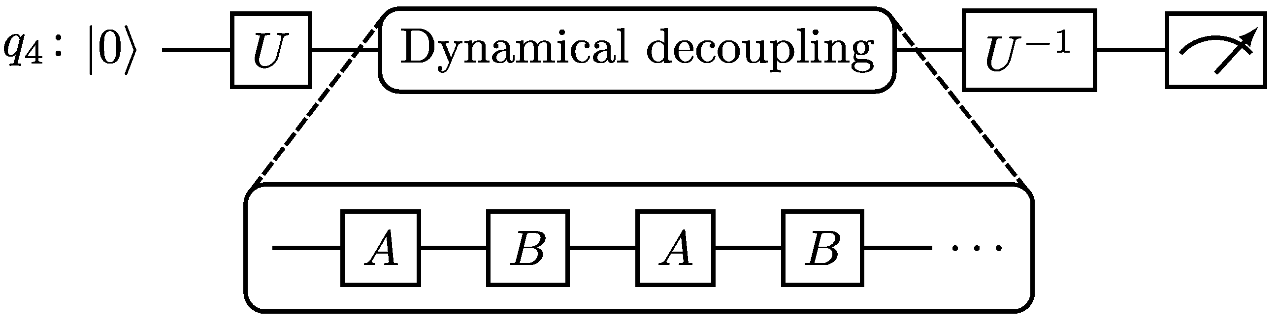
The experiment circuits can be divided into four main parts: state preparation, dynamical decoupling, state decoding, and measurement. We denote the state preparation step with the gate U, which will have a form that will depend on the state being prepared. The state decoding step will consist of applying $U^{-1}$, the inverse of the preparation gate. For the single-qubit tests, we considered the states |0⟩ and |1⟩. In this case, U will be $U=X$ for the |1⟩ state, while no U gate will be required for the |0⟩ state. The circuits used for carrying out the single-qubit experiments are shown schematically in Figure 1.

In said figure, the $U^{-1}$ gate theoretically returns the qubit back to the |0⟩ state. With it, if we obtain the |0⟩ state at the measurement part, we know that the state has been successfully protected. Therefore, we will consider the following fidelity metric for the single-qubit experiments:

$${\mathcal{F}}_{sq}={\displaystyle \frac{C_0}{N_s}},$$

(2)

where $N_s$ is the number of shots (i.e., the number of times that the circuit is executed) and $C_0$ is the number of those shots in which we measure the |0⟩ state (i.e., the |0⟩ counts). This can be interpreted as ${\mathcal{F}}_{sq}$ representing the survival probability of the state.

It is important to note that, in Figure 1, we do not introduce any time interval between the sequence gates. This was done in order to stay as close as possible to the ideal conditions of dynamical decoupling, which requires frequent pulses. In addition, free evolution is equivalent to the $A=B=I$ case (an IIII sequence), as the identity gate is implemented as a waiting time interval in which nothing is done to the qubit.

Visualizing the pulse schedule of the circuits with Qiskit [20], we can check that there is indeed no undesired wait time between the sequence pulses, unless explicitly specified. Thus, the sequence duration will be given by the duration of all the gates. As the number of $AB$ gate pairs must be even, we used 4 gate blocks of the form $ABAB$ to build the dynamical decoupling parts. To construct the circuits, we set a given sequence time $\tau$. Considering that ${\tau }_b=2({\tau }_A+{\tau }_B)$ is the time duration of a 4-gate block, with ${\tau }_A$ and ${\tau }_B$ being the duration of the A and B gates, respectively, the number $N_b$ of blocks to be put in the circuit will be given by the following expression:

$$N_b=⌊{\displaystyle \frac{\tau }{{\tau }_b}}⌋.$$

(3)

The resulting sequence may have a total duration different than $\tau$, due to the floor rounding operation in Equation (3). Thus, we calculate the real sequence time ${\tau }_s$ used when plotting the results as

$${\tau }_s=N_b{\tau }_b.$$

(4)

All of this is performed in order to compare results from different gate sequences at similar points in time, as different types of gates may have different durations. The duration of the gates used for the sequences is shown in

Table 1. Duration of the identity gate I and the different Pauli gates used for building the circuit sequences. Here, $dt=2/9$ ns is the finest time resolution of the pulses and the cycle time of the system [19,20]. The duration in nanoseconds is rounded to two decimal places.

Gate Name	Duration in $\mathit{d}\mathit{t}$ Units	Duration in Nanoseconds
I	160	$35.56$
$\sqrt{X}$	160	$35.56$
X	160	$35.56$
Y	320	$71.11$
Z	0	0

, including the duration of the identity gate I used for building the free evolution circuits.

In Table 1, the duration of the Y gate corresponds to its raw decomposition into native basis gates:

$$Y=R_z\left(\frac{\pi }{2}\right)\sqrt{X}{R}_z\left(2\pi \right)\sqrt{X}{R}_z\left(\frac{7\pi }{2}\right),$$

(5)

which is applied from left to right and is the form used in the circuit sequences. As the Z gate is implemented virtually as an offset added to pulsed gates such as the X or $\sqrt{X}$ gates [21], it has an effective duration of 0 ns [15,19,20,21]. It is decomposed into native gates as $Z=R_z\left(-\pi \right)$ [20]. In addition, it is also important to note that sequences consisting only of virtual Z gates and optional wait intervals would not be effective for dynamical decoupling. This is because these virtual gates are not implemented natively as a microwave pulse as dynamical decoupling requires. A sequence of offsets applied to the wave generator would not produce any effect on the physical qubits if no subsequent pulses are sent to them.

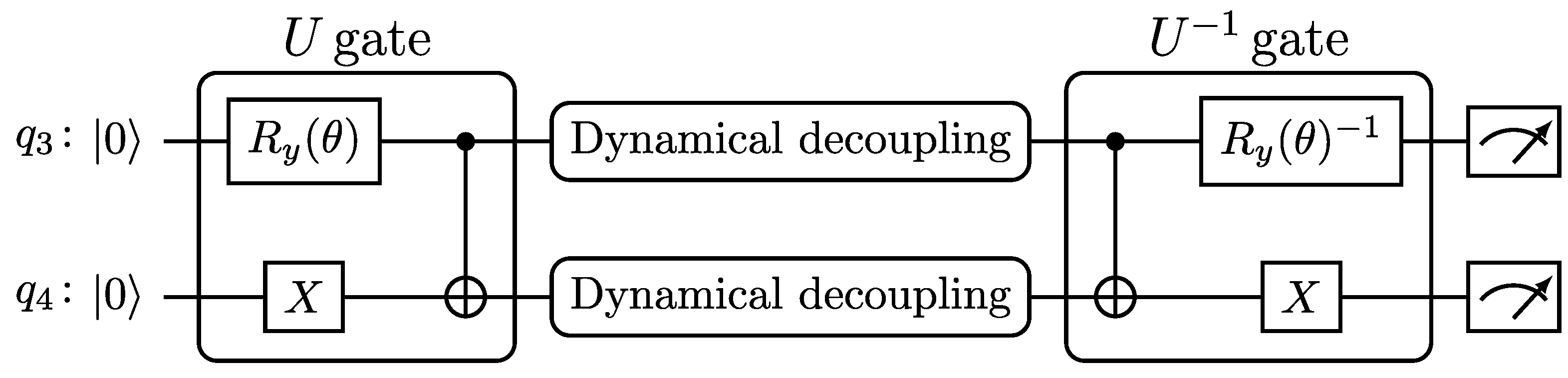
In the two-qubit tests, we followed the same circuit building approach. We started by considering the maximally entangled Bell states $|{\beta }_{ij}⟩$ previously shown in Equation (1). The circuits used for carrying out dynamical decoupling tests with them are presented in Figure 2.

The fidelity metric considered for this case is very similar to the one used in the single-qubit case. The difference is that, this time, its expression depends on the |00⟩ state counts denoted as $C_{00}$. Thus, the two-qubit fidelity will be

$${\mathcal{F}}_{tq}={\displaystyle \frac{C_{00}}{N_s}}.$$

(6)

In addition to the Bell states, we considered the more general case with states of the form

$$|{\psi }_{ab}⟩=a|01⟩+b|10⟩.$$

(7)

The real probability amplitudes a and b are related through the normalization condition $a^2+b^2=1$. Therefore, we took a as the independent parameter and considered equidistant values in the $[0,1]$ and $[-1,0]$ intervals. b will always remain positive.

These states can be prepared with the help of the $R_y\left(\theta \right)$ gates, which are rotations of angle $\theta$ about the y axis of the Bloch sphere and are implemented as [20]

$$R_y\left(\theta \right)=\left(\begin{array}{cc}cos\left(\theta /2\right)& -sin\left(\theta /2\right)\\ sin\left(\theta /2\right)& cos\left(\theta /2\right)\end{array}\right).$$

(8)

The decomposition of the $R_y\left(\theta \right)$ gate into native basis gates can be obtained using Qiskit [20]. The decomposition, as the one of the Y gate, follows the general SU(2) form presented in [21], and it is

$$R_y\left(\theta \right)=R_z\left(0\right)\sqrt{X}{R}_z(\pi -\theta )\sqrt{X}{R}_z\left(3\pi \right).$$

(9)

Having that

$$R_y\left(\theta \right)|0⟩=\left(\begin{array}{cc}cos\left(\theta /2\right)& -sin\left(\theta /2\right)\\ sin\left(\theta /2\right)& cos\left(\theta /2\right)\end{array}\right)\left(\begin{array}{c}1\\ 0\end{array}\right)=cos\left({\displaystyle \frac{\theta }{2}}\right)|0⟩+sin\left({\displaystyle \frac{\theta }{2}}\right)|1⟩,$$

(10)

we considered $a=cos(\theta /2)$ and $b=sin(\theta /2)$. This way, a and b are real and satisfy $a^2+b^2=1$. To obtain the circuits used, we considered a as the independent parameter and generated a set of 30 evenly spaced values of a between $a=0$ and $a=1$, as previously mentioned. From this, we obtained the $\theta$ values by using $\theta =2arccos\left(a\right)$. Then, we repeated the process with the case where a and b have opposite signs with $-1\le a\le 0$.

It is important to mention the ket ordering convention used by Qiskit. For example, considering Qubits 3 ($q_3$) and 4 ($q_4$), with the former being in the |1⟩ state and the latter in the |0⟩ state, the notation of the Qiskit ket would be $|q_4{q}_3⟩=|01⟩$. That is, the state label of Qubit 4 is written first inside the ket. In Equation (7), we used the convention followed in the classical textbook [18], where we would have $|q_3{q}_4⟩=|10⟩$ with the state label of Qubit 3 written first. As we worked with Qiskit, we used its ket ordering convention. Thus, the $a=1$ case would correspond to $|{\psi }_{ab}⟩=|10⟩$ using the ket ordering from Qiskit.

With this in mind, we can write the U gate that prepares the $|{\psi }_{ab}⟩$ state and build the circuits as shown in Figure 3. For these experiments we also considered the two-qubit fidelity expression shown in Equation (6).

In all the circuits from the three situations mentioned above (single-qubit, Bell states, and $|{\psi }_{ab}⟩$ states), we used $N_s=2^{13}=8192$ shots for running each circuit and repeated each experiment 10 times to obtain an idea of the variability of the results. From the values obtained during the repetitions, we set the maximum and minimum values as the error bar limits, and the plotted points represent the average values obtained in the repetitions. In the case of the $|{\psi }_{ab}⟩$ states, the results are shown in the form of heat map landscapes. In said heat maps, the error bars cannot be directly shown as in the other plots. Thus, we show the “fidelity error amplitude” obtained as the difference between the upper and lower limits of the respective error bar. This was done to keep track of the variability of the results.

3. Results and Discussions

We begin the Results Section by presenting the single-qubit case, following with the Bell two-qubit case, and lastly, with the more general $|{\psi }_{ab}⟩$ two-qubit case. In the two former cases and with the |10⟩ and |01⟩ states, we performed exponential decay fits of the data. These fits have the form

$$F\left(\tau \right)=e^{-\tau /T}+C,$$

(11)

where $\tau$ is the duration of the sequence (sequence time), T is the time scale of the decay, and C is a fitting constant. The values of all the fit parameters are available in Appendix A.

The results of the single-qubit experiments are shown in Figure 4. In this figure, we see that applying the dynamical decoupling sequences on the ground state |0⟩ induces a fidelity decay in comparison with the free evolution given by the I-only sequence. This alone would already mean that the experimental pulses are not suitable for this particular simple dynamical decoupling approach, as an unknown state would not be able to be protected without taking further care. With the |1⟩ state, the decoherence process is so quick that the application of the sequences slows down the process, even with the experimental imperfections of the pulses. It can also be noted that the evolution under the XYXY sequence seems to be equivalent in both states. This may be due to the |0⟩ and |1⟩ states’ continuous flipping on the Bloch sphere, as both states travel between the poles of the Bloch sphere during the execution of the sequences.

The results with the ground state |0⟩ seen in Figure 4 are consistent with the results of previous works on the subject [10]. In [10], it is indicated that dynamical decoupling is worse than free evolution for states close to the ground state in this kind of device. This means that the application of dynamical decoupling pulse sequences is not useful at all for preserving the ground state |0⟩ in time.

In addition, it has been demonstrated that the quantum Zeno effect is equivalent to “bang-bang” decoupling (i.e., dynamical decoupling) [12]. Thus, a possible hypothesis would be that the induced decay obtained for the |0⟩ state is the product of different factors. These factors may be the accumulation of pulse errors, the magnitude of the noise components uncorrected by the real pulse sequences, and an “anti-Zeno-like” effect due to the pulses not being short enough. The trajectory of the state on the Bloch sphere during the execution of the sequences is another of these factors, as states closer to the ground state |0⟩ are naturally more stable than the ones closer to the excited state |1⟩ [6,10], which is susceptible to thermal relaxation.

All of this indicates that simple dynamical decoupling cannot be applied in the device in order to fully protect an unknown state without further care for the sequence design. However, we observed that dynamical decoupling is able to slow down the fidelity decay of other states considered.

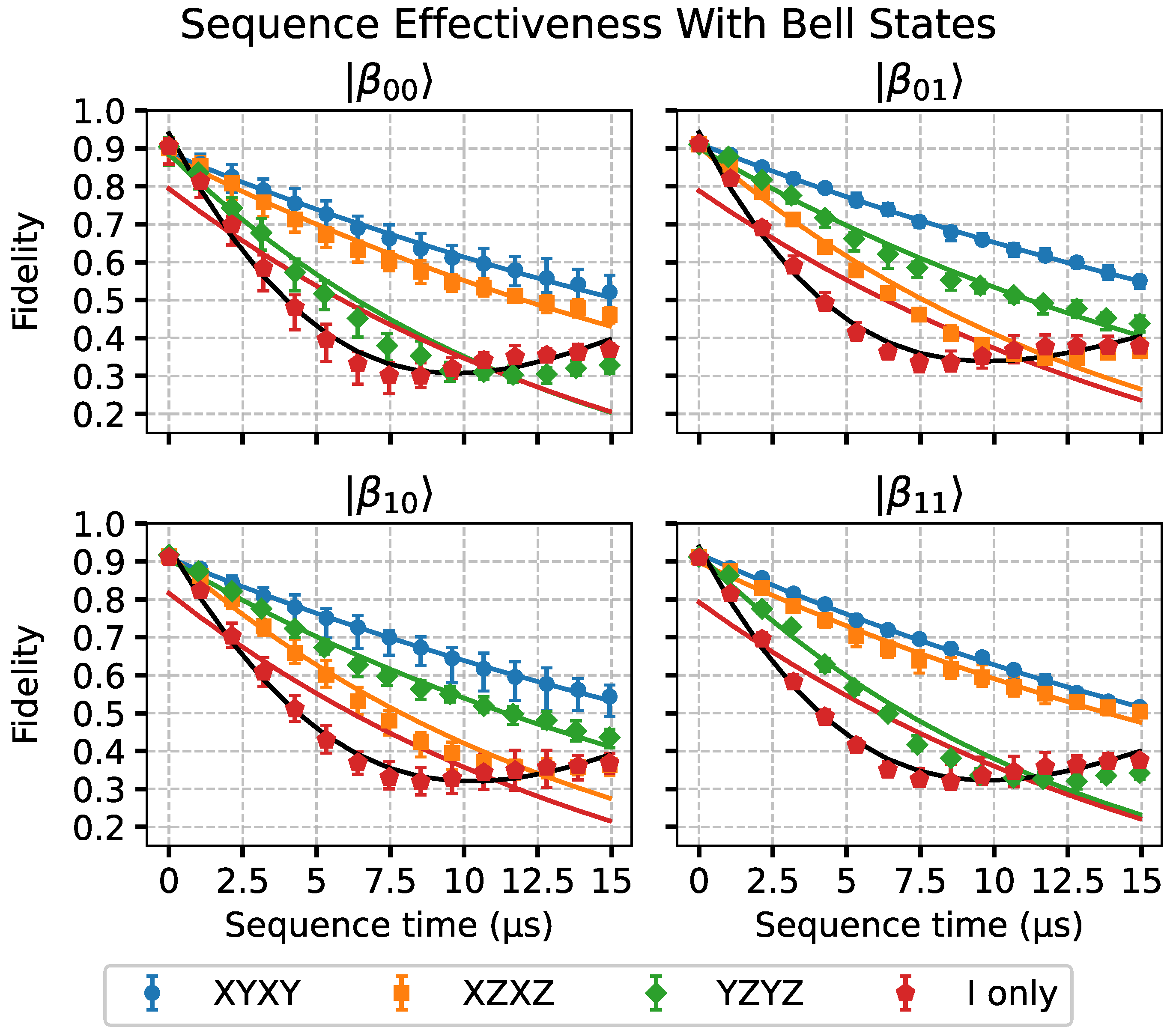
In Figure 5, the results with the Bell states are presented. In said figure, we performed an additional fit of the free evolution data. This fit follows a damped cosine expression such as

$$F_{\mathit{free}}\left(\tau \right)=e^{-\tau /T}cos\left(2\pi f\tau +\varphi \right)+C,$$

(12)

where $\tau$, T, and C have the same meaning as in Equation (11) and f and $\varphi$ are also fitting parameters representing a frequency and a phase, respectively. We can note that, for long sequence times, the dynamical decoupling pulses will not be better than free evolution. In this large sequence time region, it can be noted that the free evolution dynamics shows non-Markovian behavior, as the fidelity points do not adjust well to the exponential decay behavior. This makes the damped cosine fit a better choice than the exponential decay fit to describe the data. We obtained that the dynamical decoupling sequences mitigate the non-Markovian component of the two-qubit evolution dynamics, as observed in [10], for single-qubit states in an IBMQ device. This was achieved at least within the sequence times considered. In [22], it is discussed that these non-Markovian effects may arise from different sources, such as: noise from the external pulse controls, residual Hamiltonian terms, slow environmental fluctuations, undesired qubit crosstalk, or coupling to magnetic impurities. However, for short times, there is a clear benefit in using the sequences with these maximally entangled states. It can also be observed that, with all four states, the XYXY sequence is the best among the three.

Lastly, in Figure 6, Figure 7 and Figure 8, the results from the more general case with the two-qubit $|{\psi }_{ab}⟩$ states are presented. In Figure 6, we can see the results considering |10⟩ and |01⟩ as initial states. These kets are written using the Qiskit ket ordering notation [20]. The |10⟩ state would correspond to the $a=0$ case, while |01⟩ would correspond to $a=1$. We can observe that, for these separable quantum states, there seems to be no clear advantage in using dynamical decoupling with respect to free evolution. However, for the |01⟩ state, the decay slightly slows down with the XYXY sequence.

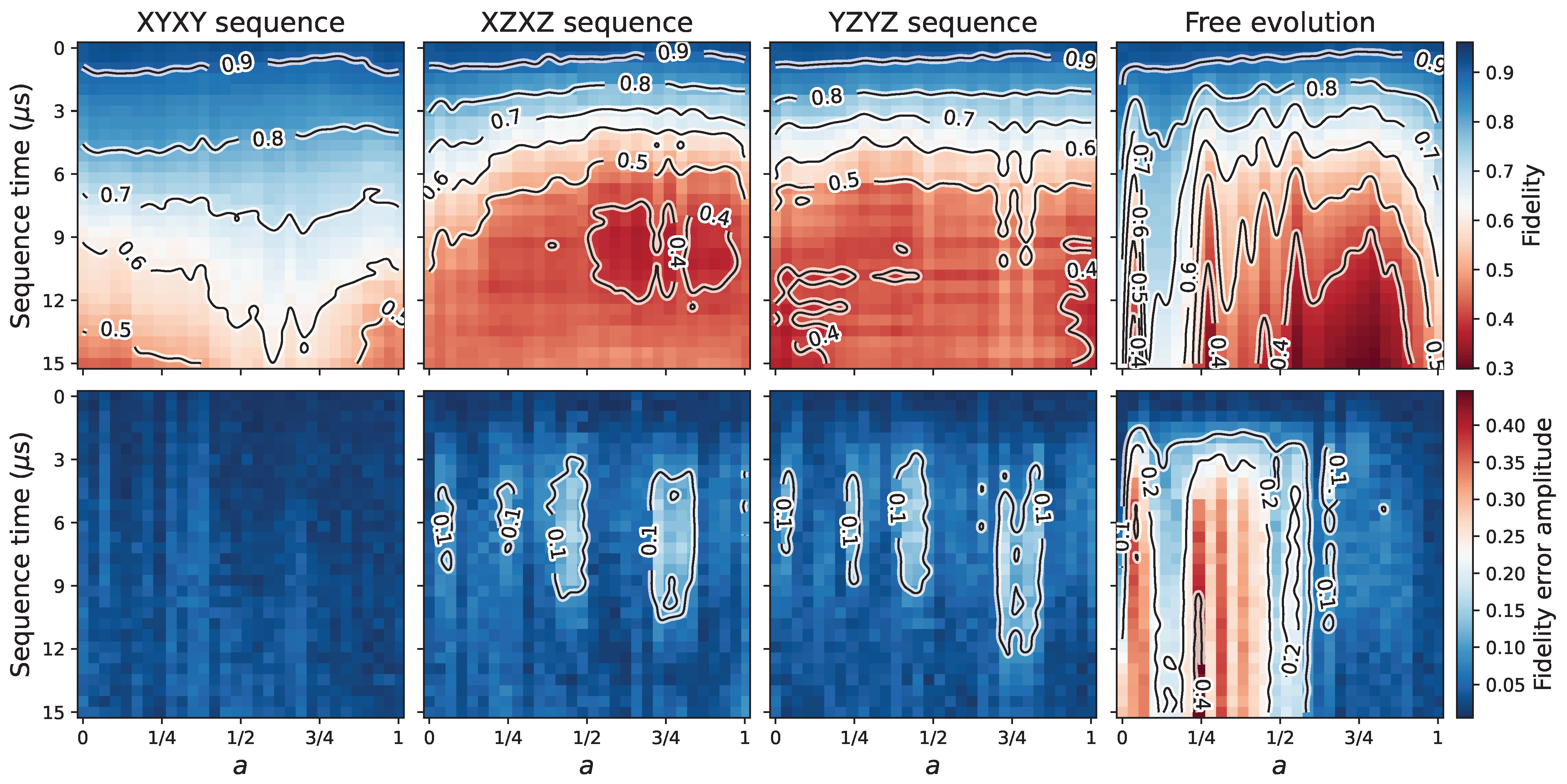
In Figure 7 and Figure 8, the $|{\beta }_{01}⟩$ and $|{\beta }_{11}⟩$ states would correspond to the $a=1/\sqrt{2}\approx 0.71$ and $a=-1/\sqrt{2}\approx -0.71$ values, respectively. At the top row of the subplots of these figures, the fidelity data represented using color are shown as a function of the a parameter and the sequence time. At the bottom row of the subplots, the figures show the amplitude of the error bars, named “fidelity error amplitude”, as explained at the end of the Section 2. In both figures, we used the same limits for the color bars of the “fidelity” plots. That is, the maximum and minimum values were taken considering the fidelity data from both positive a and negative a situations for comparison purposes. The contours on the figures are shown qualitatively, in order to make the reading of the data easier. It is also important to mention that the results in Figure 7 and Figure 8 will depend on factors such as the device, the qubits used, and their robustness against environmental noise.

The first thing that we can note from these results is that the XYXY sequence is generally more beneficial than the other sequences and free evolution. However, we can observe that free evolution is better than dynamical decoupling for sates close to the $a\approx 0$ states. Nevertheless, roughly speaking, the states most benefiting from this simple decoupling approach are the ones with a values approximately in the $\pm [1/4,1]$ intervals with the XYXY sequence.

The largest variability of the results (i.e., fidelity error amplitude) was obtained for the positive a free evolution case (Figure 7), for states with $0\le a\lesssim 1/2$. In Figure 7, with the XZXZ and YZYZ sequences, the larger variability is localized in regions with centers close to the $a=0$, $a=1/4$, $a\approx 0.45$, and $a=3/4$ states. In Figure 8, we can still observe some traces of these higher variability regions. In this case, they appear mainly around the $a\approx -0.45$ and $a=-3/4$ points. Generally and with respect to free evolution, we can note that the sequences reduce the variability.

4. Conclusions

We tested the effectiveness of different sequences of native IBMQ quantum gates for dynamical decoupling. It was also shown that the XYXY gate sequence is generally the best one among the three universal sequences that we applied on the ibmq_lima device from IBMQ [19]: XYXY, XZXZ, and YZYZ. This XYXY sequence in general slows down the decay of the survival probability (i.e., the fidelity metric) of a large subset of the states considered.

No perfect quantum control against decoherence has been achieved experimentally, so an unknown quantum state will not be able to be completely protected without taking further care in the sequence design. The results show that the IBMQ native gates are currently not ideal for their use in dynamical decoupling (as can be noted, for example, with the |0⟩ state), or at least for how the technique is implemented in the present work. We hypothesize that one of the reasons for this is the duration of the gate pulses. Furthermore, a relatively long duration of the pulsed gates used as bang-bang operations may serve as an open door for the influence of an “anti-Zeno-like” effect [12]. Thermal relaxation happening during the execution of the sequences is an important factor to consider. The large amount of gate pulses used in order to achieve long wait times may also introduce additional errors due to the accumulation of the imperfections of individual pulses.

We explored the effectiveness of the three dynamical decoupling sequences considered with a relatively large collection of two-qubit states, which includes the maximally entangled Bell states and the $|{\psi }_{ab}⟩=a|10⟩+b|01⟩$ states (using Qiskit’s ket ordering convention) with real a and b parameters. These results are of interest for logical qubit encodings such as $\{{|0⟩}_L\equiv |01⟩,1_L\equiv |10⟩\}$, which may tend to be broken due to thermal relaxation to the physical |00⟩ state and where the states may have the form of $|{\psi }_{ab}⟩$. With the device and qubits used, we observed that, for states near the $a\approx 0$ region, dynamical decoupling is not useful in comparison to free evolution. Nevertheless, we also showed that states approximately in the $a\in \pm [1/4,1]$ intervals are clearly the most benefiting from the XYXY sequence, which is generally the sequence with the best performance in our case.

References

1. Lidar, D.A.; Brun, T.A. Quantum Error Correction; Cambridge University Press: Cambridge, UK, 2013. [Google Scholar] [CrossRef] [Green Version]
2. Gyongyosi, L.; Imre, S. A Survey on quantum computing technology. Comput. Sci. Rev. 2019, 31, 51–71. [Google Scholar] [CrossRef]
3. Georgescu, I. 25 years of quantum error correction. Nat. Rev. Phys. 2020, 2, 519. [Google Scholar] [CrossRef]
4. Viola, L. Introduction to quantum dynamical decoupling. In Quantum Error Correction; Lidar, D.A., Brun, T.A., Eds.; Cambridge University Press: Cambridge, UK, 2013; pp. 105–125. [Google Scholar] [CrossRef]
5. Lidar, D.A. Review of Decoherence-Free Subspaces, Noiseless Subsystems, and Dynamical Decoupling. In Quantum Information and Computation for Chemistry; John Wiley & Sons, Ltd.: New York, NY, USA, 2014; pp. 295–354. [Google Scholar] [CrossRef] [Green Version]
6. Ezzell, N.; Pokharel, B.; Tewala, L.; Quiroz, G.; Lidar, D.A. Dynamical decoupling for superconducting qubits: A performance survey. arXiv 2022, arXiv:2207.03670. [Google Scholar] [CrossRef]
7. Pokharel, B.; Lidar, D.A. Demonstration of algorithmic quantum speedup. arXiv 2022, arXiv:2207.07647. [Google Scholar] [CrossRef]
8. Wu, L.A.; Lidar, D. Quantum malware. Quantum Inf. Process. 2006, 5, 69–81. [Google Scholar] [CrossRef]
9. Smith, P.E.; Bensky, G.; Álvarez, G.A.; Kurizki, G.; Frydman, L. Shift-driven modulations of spin-echo signals. Proc. Natl. Acad. Sci. USA 2012, 109, 5958–5961. [Google Scholar] [CrossRef] [PubMed] [Green Version]
10. Pokharel, B.; Anand, N.; Fortman, B.; Lidar, D.A. Demonstration of fidelity improvement using dynamical decoupling with superconducting qubits. Phys. Rev. Lett. 2018, 121, 220502. [Google Scholar] [CrossRef] [PubMed]
11. Souza, A.M.; Álvarez, G.A.; Suter, D. Robust dynamical decoupling. Philos. Trans. R. Soc. A Math. Phys. Eng. Sci. 2012, 370, 4748–4769. [Google Scholar] [CrossRef] [PubMed] [Green Version]
12. Facchi, P.; Lidar, D.A.; Pascazio, S. Unification of dynamical decoupling and the quantum Zeno effect. Phys. Rev. A 2004, 69, 032314. [Google Scholar] [CrossRef] [Green Version]
13. Wu, L.A.; Lidar, D.A. Creating Decoherence-Free Subspaces Using Strong and Fast Pulses. Phys. Rev. Lett. 2002, 88, 207902. [Google Scholar] [CrossRef] [PubMed] [Green Version]
14. Pyshkin, P.; Luo, D.W.; Jing, J.; You, J.; Wu, L.A. Expedited holonomic quantum computation via net zero-energy-cost control in decoherence-free subspace. Sci. Rep. 2016, 6, 1–6. [Google Scholar] [CrossRef] [PubMed] [Green Version]
15. Krantz, P.; Kjaergaard, M.; Yan, F.; Orlando, T.P.; Gustavsson, S.; Oliver, W.D. A quantum engineer’s guide to superconducting qubits. Appl. Phys. Rev. 2019, 6, 021318. [Google Scholar] [CrossRef] [Green Version]
16. Tripathi, V.; Chen, H.; Khezri, M.; Yip, K.W.; Levenson-Falk, E.; Lidar, D.A. Suppression of Crosstalk in Superconducting Qubits Using Dynamical Decoupling. Phys. Rev. Appl. 2022, 18, 024068. [Google Scholar] [CrossRef]
17. Wu, L.A.; Liu, Y.X.; Nori, F. Universal existence of exact quantum state transmissions in interacting media. Phys. Rev. A 2009, 80, 042315. [Google Scholar] [CrossRef] [Green Version]
18. Nielsen, M.A.; Chuang, I.L. Quantum Computation and Quantum Information: 10th Anniversary Edition; Cambridge University Press: Cambridge, UK, 2010. [Google Scholar] [CrossRef] [Green Version]
19. IBM Quantum. 2022. Available online: https://quantum-computing.ibm.com/ (accessed on 11 October 2022).
20. Anis, M.S.; Abraham, H.; AduOffei, R.A.; Agliardi, G.; Aharoni, M.; Akhalwaya, I.; Aleksandrowicz, G.; Alexander, T.; Amy, M.; Anagolum, S.; et al. Qiskit: An Open-Source Framework for Quantum Computing. 2022. Available online: https://zenodo.org/record/6560959#.Y6kVXhVBxPY (accessed on 11 October 2022).
21. McKay, D.C.; Wood, C.J.; Sheldon, S.; Chow, J.M.; Gambetta, J.M. Efficient Z gates for quantum computing. Phys. Rev. A 2017, 96, 022330. [Google Scholar] [CrossRef] [Green Version]
22. Zhang, H.; Pokharel, B.; Levenson-Falk, E.; Lidar, D. Predicting Non-Markovian Superconducting-Qubit Dynamics from Tomographic Reconstruction. Phys. Rev. Appl. 2022, 17, 054018. [Google Scholar] [CrossRef]
23. Newville, M.; Otten, R.; Nelson, A.; Ingargiola, A.; Stensitzki, T.; Allan, D.; Fox, A.; Carter, F.; Michał; Osborn, R.; et al. lmfit/lmfit-py: 1.0.3. 2021. Available online: https://zenodo.org/record/5570790#.Y6kVJhVBxPY (accessed on 11 October 2022).
Figure 1. Circuits used for the single-qubit state experiments. The q 4 tag indicates that Qubit 4 is being used. The qubit starts in the |0⟩ state, and the U gate represents the preparation step. A and B correspond to the unitary gates that form the sequence, and the number of A B pairs must be even. For example, A = X and B = Y for the XYXY sequence.
Symmetry 15 00062 g001
Figure 2. Circuits used for the two-qubit state experiments with Bell states. The i , j = 0 , 1 powers on the X gates correspond to the indexes of the | β i j state being prepared, and H is the Hadamard gate. The general structure of the circuit is the same as the one shown in Figure 1.
Symmetry 15 00062 g002
Figure 3. Circuits used for the two-qubit state experiments with the | ψ a b states. The circuit is analogous to the one shown in Figure 2, but with a different preparation gate U.
Symmetry 15 00062 g003
Figure 4. Results of the single-qubit case. Here, the fidelity data are shown as a function of the duration of the dynamical decoupling sequences (sequence time). Each state considered is indicated as the title of the respective subplot. Free evolution is represented by the I-only sequence.
Symmetry 15 00062 g004
Figure 5. Results of the two-qubit case with Bell states using Qubits 3 and 4 of the ibmq_lima quantum processing unit. The fidelity data are shown as a function of the duration of the sequences. An additional damped cosine fit of the data, indicated in black color, was performed in the free evolution case (I-only sequence).
Symmetry 15 00062 g005
Figure 6. Results of the two-qubit case with the |10⟩ and |01⟩ states. Fidelity data are shown as a function of the duration of the dynamical decoupling sequences. Exponential decay fits of the data are also shown. The states are noted following the Qiskit ket ordering notation, as mentioned in the Section 2 (i.e., | q 4 q 3 ). |10⟩ corresponds to a = 0 and |01⟩ to a = 1 .
Symmetry 15 00062 g006
Figure 7. Results of the | ψ a b | tests using Qubits 3 and 4 of the ibmq_lima quantum processing unit and positive values of the a parameter. At the top row of the subplots, the fidelity data represented in color are shown as a function of the sequence time and the a parameter defining | ψ a b . At the bottom row, the amplitude of the error bars (denoted as “fidelity error amplitude”) of the top row subplots is shown. The qualitative contour lines are shown to facilitate reading the values of the plots.
Symmetry 15 00062 g007
Figure 8. Analogous to Figure 7, but considering negative values of a. Both figures share the same color bar limits in the fidelity subplots. These limits were taken from the minimum and maximum values of the combined fidelity data. This was performed to facilitate the comparison of the fidelity results from both figures.
Symmetry 15 00062 g008