

Absolute 3D Human Pose Estimation Using Noise-Aware Radial Distance Predictions

Abstract
1. Introduction
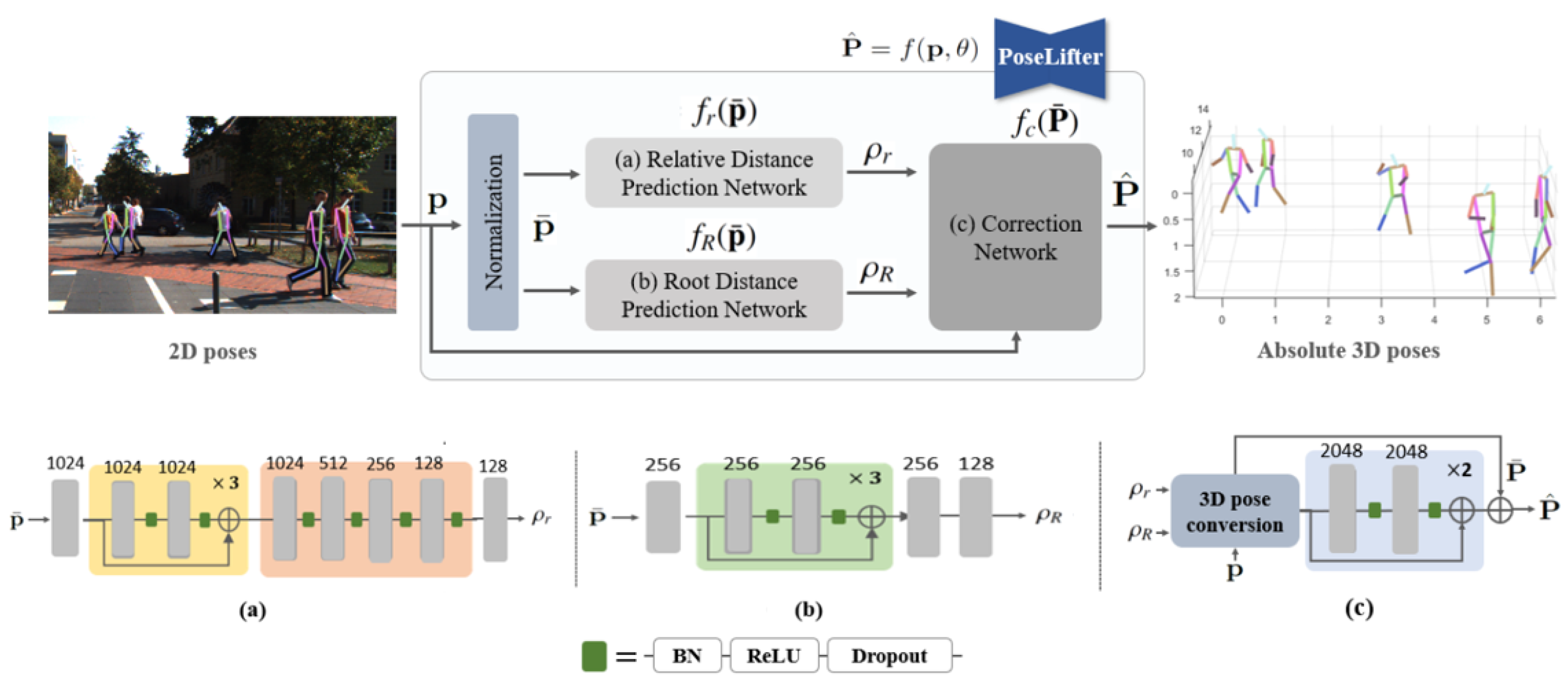
- The previous methods directly perceive absolute 3D joints from 2D joint keypoints as input i.e., , but our method predicts both one-dimensional root distance and root-relative distance of other joints using two regression networks i.e., . Afterwards, a simple 3D conversion function computes an initial absolute 3D pose using the input and the predicted distances. Thanks to lower-dimensional output, we can efficiently reduce the number of network parameters while keeping the performance competitive with state-of-the-art methods. This is because the radial distance prediction indirectly avoids perspective projection errors by disentangling the depth ambiguity caused by horizontal and vertical components.
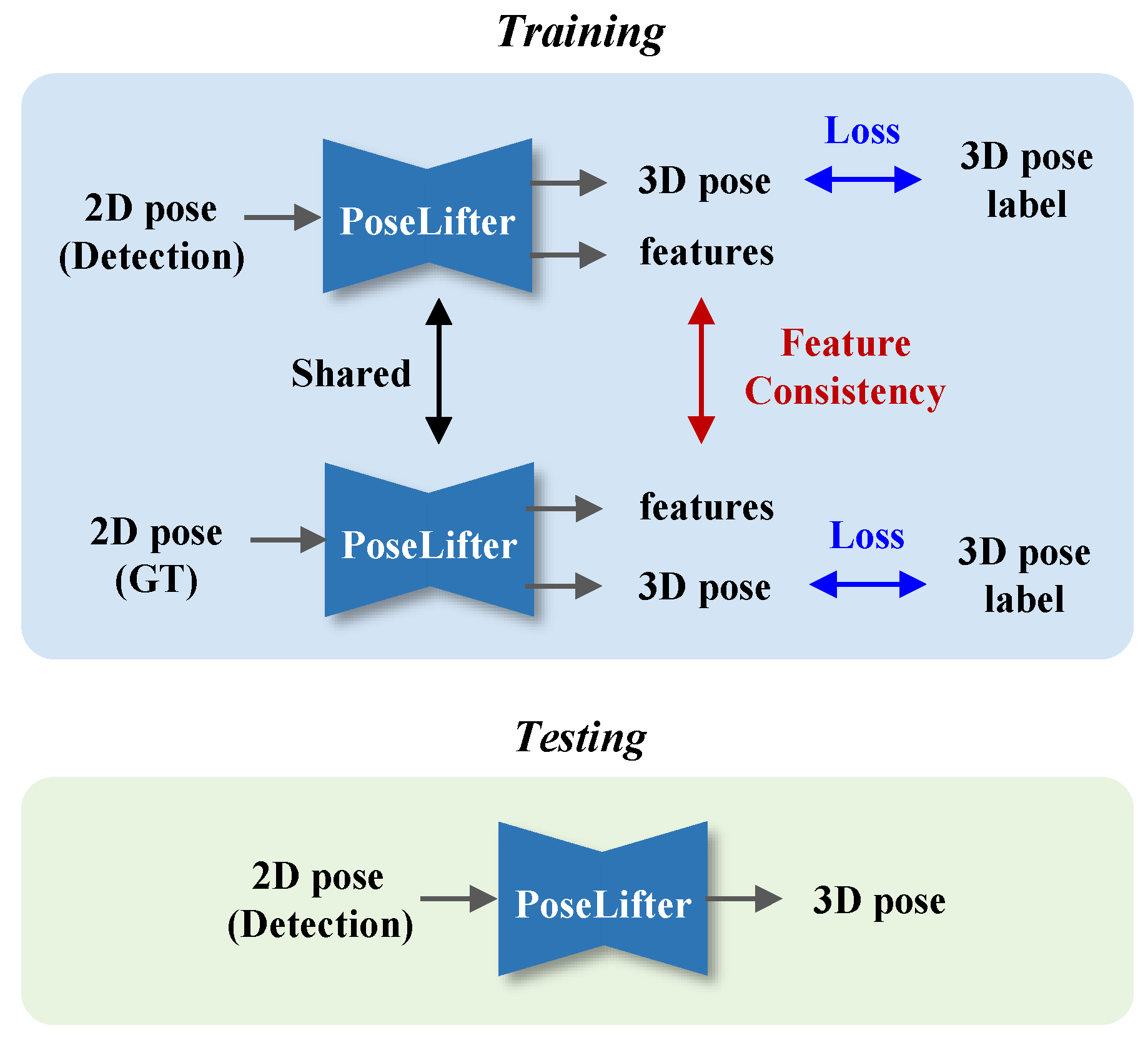
- We propose to use a correction network to reduce the absolute 3D pose uncertainties, affected by input noise. When the ground truth of 2D joint keypoints are available, we adopt a Siamese architecture [28] that shares the network for noisy and clean inputs. By applying the feature consistency for different inputs, we reduce the influence of detection noise implicitly. Contrarily to our approach, the existing study [20] augments training data using synthesized errors generated from the error statistics.
2. Related Work
2.1. Absolute 2D-to-3D Pose Lifting
2.2. Root-Relative 2D-to-3D Pose Lifting
3. Methodology
3.1. Problem Formulation
3.2. Absolute 3D Pose from Distances
3.3. Proposed Pipeline
3.4. Training via Siamese Architecture
4. Experimental Results
4.1. Implementation
4.2. Datasets
4.3. Evaluation Metrics
4.4. Ablation Study
4.5. Evaluation on Different Parameter Sizes
4.6. Quantitative and Qualitative Results
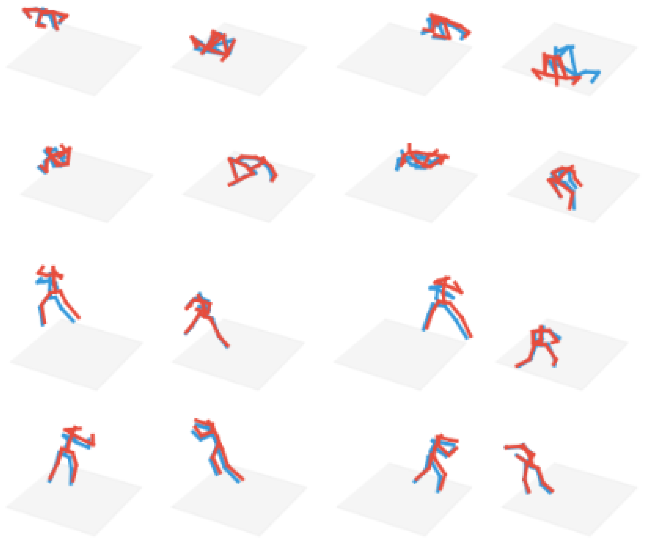
4.6.1. Human3.6M
4.6.2. MPI-3DHP
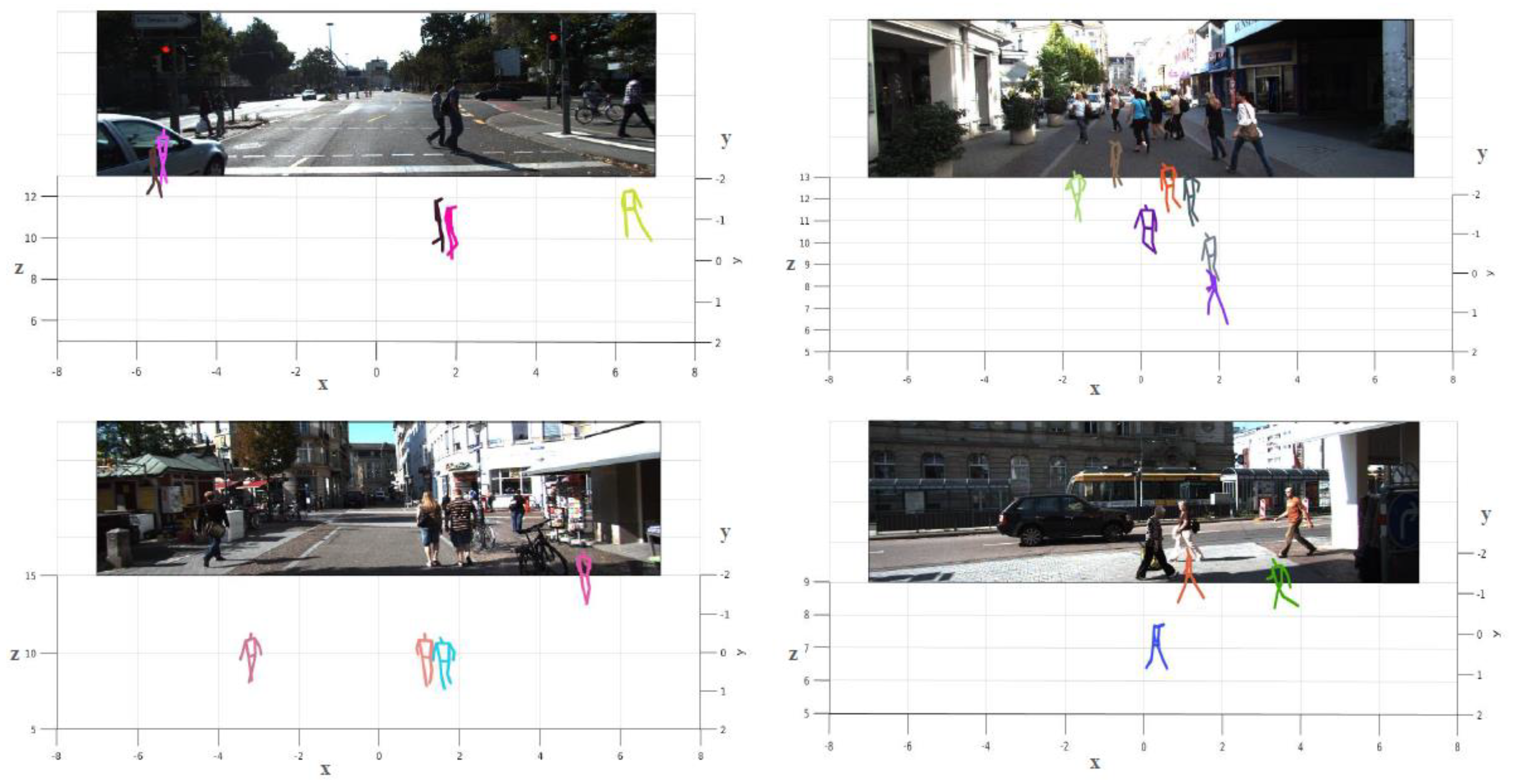
4.6.3. KITTI
4.7. Limitations
5. Conclusions
Author Contributions
Funding
Institutional Review Board Statement
Informed Consent Statement
Data Availability Statement
Acknowledgments
Conflicts of Interest
References
- Optitrack. Available online: https://www.optitrack.com/ (accessed on 1 January 2022).
- Qualisys. Available online: https://www.qualisys.com/ (accessed on 1 January 2022).
- Liu, W.; Bao, Q.; Sun, Y.; Mei, T. Recent Advances in Monocular 2D and 3D Human Pose Estimation: A Deep Learning Perspective. arXiv 2021, arXiv:2104.11536. [Google Scholar] [CrossRef]
- Wu, Y.; Ma, S.; Zhang, D.; Sun, J. 3D Capsule Hand Pose Estimation Network Based on Structural Relationship Information. Symmetry 2020, 12, 1636. [Google Scholar] [CrossRef]
- Moon, G.; Chang, J.Y.; Lee, K.M. Camera distance-aware top-down approach for 3d multi-person pose estimation from a single rgb image. In Proceedings of the ICCV, Seoul, Republic of Korea, 27 October–2 November 2019. [Google Scholar]
- Lin, J.; Lee, G.H. HDNet: Human depth estimation for multi-person camera-space localization. In Proceedings of the ECCV, Seattle, WA, USA, 13–19 June 2020. [Google Scholar]
- Cheng, Y.; Wang, B.; Yang, B.; Tan, R.T. Graph and temporal convolutional networks for 3d multi-person pose estimation in monocular videos. In Proceedings of the AAAI, Palo Alto, CA, USA, 22–24 March 2021. [Google Scholar]
- Cheng, Y.; Wang, B.; Yang, B.T.; Tan, R. Monocular 3D Multi-Person Pose Estimation by Integrating Top-Down and Bottom-Up Networks. In Proceedings of the CVPR, Nashville, TN, USA, 20–25 June 2021. [Google Scholar]
- Chen, Y.; Wang, Z.; Peng, Y.; Zhang, Z.; Yu, G.; Sun, J. Cascaded pyramid network for multi-person pose estimation. In Proceedings of the CVPR, Salt Lake City, UT, USA, 18–23 June 2018. [Google Scholar]
- Kreiss, S.; Bertoni, L.; Alahi, A. PifPaf: Composite fields for human pose estimation. In Proceedings of the CVPR, Long Beach, CA, USA, 15–20 June 2019. [Google Scholar]
- Cao, Z.; Hidalgo Martinez, G.; Simon, T.; Wei, S.; Sheikh, Y.A. OpenPose: Realtime multi-person 2D pose estimation using part affinity fields. IEEE Trans. Pattern Anal. Mach. Intell. 2019, 43, 172–186. [Google Scholar] [CrossRef]
- Martinez, J.; Hossain, R.; Romero, J.; Little, J.J. A Simple yet effective baseline for 3d human pose estimation. In Proceedings of the ICCV, Venice, Italy, 22–29 October 2017. [Google Scholar]
- Tome, D.; Russell, C.; Agapito, L. Lifting from the deep: Convolutional 3d pose estimation from a single image. In Proceedings of the CVPR, Honolulu, HI, USA, 21–26 July 2017. [Google Scholar]
- Fang, H.S.; Xu, Y.; Wang, W.; Liu, X.; Zhu, S.C. Learning pose grammar to encode human body configuration for 3d pose estimation. In Proceedings of the AAAI, New Orleans, LA, USA, 2–7 February 2018. [Google Scholar]
- Wang, M.; Chen, X.; Liu, W.; Qian, C.; Lin, L.; Ma, L. DRPose3D: Depth ranking in 3d human pose estimation. In Proceedings of the IJCAI, Stockholm, Sweden, 13–19 July 2018. [Google Scholar]
- Li, Y.; Li, K.; Jiang, S.; Zhang, Z.; Huang, C.; Da X., R.Y. Geometry-driven self-supervised method for 3D human pose estimation. In Proceedings of the AAAI, New York, NY, USA, 7–12 February 2020. [Google Scholar]
- Liu, S.; Lv, P.; Zhang, Y.; Fu, J.; Cheng, J.; Li, W.; Zhou, B.; Xu, M. Semi-dynamic hypergraph neural network for 3d pose estimation. In Proceedings of the IJCAI, Yokohama, Japan, 7–15 January 2020. [Google Scholar]
- Zhan, Y.; Li, F.; Weng, R.; Choi, W. Ray3D: Ray-based 3D human pose estimation for monocular absolute 3D localization. In Proceedings of the CVPR, New Orleans, LA, USA, 19–20 June 2022. [Google Scholar]
- Li, S.; Ke, L.; Pratama, K.; Tai, Y.; Tang, C.; Cheng, K.T. Cascaded deep monocular 3d human pose estimation with evolutionary training data. In Proceedings of the CVPR, Seattle, WA, USA, 16–18 June 2020. [Google Scholar]
- Chang, J.Y.; Moon, G.; Lee, K.M. PoseLifter: Absolute 3d human pose lifting network from a single noisy 2D human pose. arXiv 2019, arXiv:1910.12029. [Google Scholar]
- Bertoni, L.; Kreiss, S.; Alahi, A. MonoLoco: Monocular 3d pedestrian localization and uncertainty estimation. In Proceedings of the ICCV, Seoul, Republic of Korea, 27 October–2 November 2019. [Google Scholar]
- Bertoni, L.; Kreiss, S.; Alahi, A. Perceiving Humans: From Monocular 3D Localization to Social Distancing. IEEE Trans. Intell. Trans. Sys. 2021, 23, 7401–7418. [Google Scholar] [CrossRef]
- Mehta, D.; Rhodin, H.; Casas, D.; Fua, P.; Sotnychenko, O.; Xu, W.; Theobalt, C. Monocular 3d human pose estimation in the wild using improved CNN supervision. In Proceedings of the 3DV, Qingdao, China, 10–12 October 2017. [Google Scholar]
- Pavlakos, G.; Zhou, X.; Derpanis, K.G.; Daniilidis, K. Coarse-to-fine volumetric prediction for single-image 3D human pose. In Proceedings of the CVPR, Honolulu, HI, USA, 21–26 July 2017. [Google Scholar]
- Tekin, B.; Rozantsev, A.; Lepetit, V.; Fua, P. Direct prediction of 3d body poses from motion compensated sequences. In Proceedings of the CVPR, Las Vegas, NV, USA, 27–30 June 2016. [Google Scholar]
- Sun, X.; Xiao, B.; Wei, F.; Liang, S.; Wei, Y. Integral human pose regression. In Proceedings of the ECCV, Munich, Germany, 8–14 September 2018. [Google Scholar]
- Habibie, I.; Xu, W.; Mehta, D.; Pons-Moll, G.; Theobalt, C. In the wild human pose estimation using explicit 2d features and intermediate 3d representations. In Proceedings of the CVPR, Long Beach, CA, USA, 15–20 June 2019. [Google Scholar]
- Chopra, S.; Hadsell, R.; LeCun, Y. Learning a similarity metric discriminatively, with application to face verification. In Proceedings of the CVPR, Washington, DC, USA, 20–26 June 2005. [Google Scholar]
- Akhter, I.; Black, M.J. Pose-conditioned joint angle limits for 3D human pose reconstruction. In Proceedings of the CVPR, Boston, MA, USA, 7–12 June 2015. [Google Scholar]
- Moreno-Noguer, F. 3d human pose estimation from a single image via distance matrix regression. In Proceedings of the CVPR, Honolulu, HI, USA, 21–26 July 2017. [Google Scholar]
- Sun, X.; Shang, J.; Liang, S.; Wei, Y. Compositional human pose regression. In Proceedings of the ICCV, Venice, Italy, 22–29 October 2017. [Google Scholar]
- Pavllo, D.; Feichtenhofer, C.; Grangier, D.; Auli, M. 3D Human Pose Estimation in Video With Temporal Convolutions and Semi-Supervised Training. In Proceedings of the CVPR, Long Beach, CA, USA, 15–20 June 2019. [Google Scholar]
- Sun, J.; Wang, M.; Zhao, X.; Zhang, D. Multi-View Pose Generator Based on Deep Learning for Monocular 3D Human Pose Estimation. Symmetry 2020, 12, 1116. [Google Scholar] [CrossRef]
- Kipf, T.N.; Welling, M. Semi-supervised classification with graph convolutional networks. arXiv 2016, arXiv:1609.02907. [Google Scholar]
- Shan, W.; Lu, H.; Wang, S.; Zhang, X.; Gao, W. Improving robustness and accuracy via relative information encoding in 3D human pose estimation. In Proceedings of the ACM MM, New York, NY, USA, 20–24 October 2021. [Google Scholar]
- Zheng, C.; Zhu, S.; Mendieta, M.; Yang, T.; Chen, C.; Ding, Z. 3d human pose estimation with spatial and temporal transformers. In Proceedings of the ICCV, Montreal, QC, Canada, 10–17 October 2021. [Google Scholar]
- Li, S.; Chan, A.B. 3d human pose estimation from monocular images with deep convolutional neural network. In Proceedings of the ACCV, Singapore, 1–5 November 2014. [Google Scholar]
- Zhou, X.; Zhu, M.; Leonardos, S.; Derpanis, K.; Daniilidis, K. Sparseness meets deepness: 3d human pose estimation from monocular video. In Proceedings of the CVPR, Las Vegas, NV, USA, 27–30 June 2016. [Google Scholar]
- Arnab, A.; Doersch, C.; Zisserman, A. Exploiting temporal context for 3D human pose estimation in the wild. In Proceedings of the CVPR, Long Beach, CA, USA, 15–20 June 2019. [Google Scholar]
- Kingma, D.P.; Jimmy, B. Adam: A Method for Stochastic Optimization. In Proceedings of the ICLR, San Diego, CA, USA, 7–9 May 2015. [Google Scholar]
- He, K.; Zhang, X.; Ren, S.; Sun, J. Delving deep into rectifiers: Surpassing human-level performance on imagenet classification. In Proceedings of the ICCV, Santiago, Chile, 7–13 December 2015. [Google Scholar]
- Geiger, A.; Lenz, P.; Stiller, C.; Urtasun, R. Vision meets robotics: The kitti dataset. Int. J. Rob. Res. 2013, 32, 1231–1237. [Google Scholar] [CrossRef]
- Ionescu, C.; Papava, D.; Olaru, V.; Sminchisescu, C. Human3.6m: Large scale datasets and predictive methods for 3d human sensing in natural environments. IEEE Trans. Pattern Anal. Mach. Intell. 2014, 36, 1325–1339. [Google Scholar] [CrossRef] [PubMed]
- Mehta, D.; Sotnychenko, O.; Mueller, F.; Xu, W.; Sridhar, S.; Pons-Moll, G.; Theobalt, C. Single-shot multi-person 3d pose estimation from monocular rgb. In Proceedings of the 3DV, Verona, Italy, 5–8 September 2018. [Google Scholar]
- Yang, W.; Ouyang, W.; Wang, X.; Ren, J.; Li, H.; Wang, X. 3d human pose estimation in the wild by adversarial learning. In Proceedings of the CVPR, Salt Lake City, UT, USA, 18–23 June 2018. [Google Scholar]
- Zhou, X.; Huang, Q.; Sun, X.; Xue, X.; Wei, Y. Towards 3d human pose estimation in the wild: A weakly-supervised approach. In Proceedings of the ICCV, Venice, Italy, 22–29 October 2017. [Google Scholar]
- Luo, C.; Chu, X.; Yuille, A. Orinet: A fully convolutional network for 3d human pose estimation. arXiv 2018, arXiv:1811.04989. [Google Scholar]
- Ci, H.; Wang, C.; Ma, X.; Wang, Y. Optimizing network structure for 3d human pose estimation. In Proceedings of the CVPR, Long Beach, CA, USA, 15–20 June 2019. [Google Scholar]


| Conf. | Input | MRPE | MPJPE | P-MPJPE |
|---|---|---|---|---|
| B | CPN | 109.4 | 64.4 | 48.9 |
| +RC | CPN | 109.3 | 59.3 | 45.7 |
| +F | CPN | 107.3 | 60.6 | 46.3 |
| +RC+F | CPN | 107.2 | 58.8 | 45.2 |
| +RC+F+C | CPN | 103.2 | 56.7 | 43.1 |
| Method | MRPE | # of Parameters (M = ×106) | |||
|---|---|---|---|---|---|
| Root | Relative | Correct | Full | ||
| PoseLifter | 135.1 | - | - | - | 67.0M |
| PoseFormer | 127.7 | - | - | - | 18.2M |
| Ray3D | 105.0 | - | - | - | 45.8M |
| Ours w/o C | 107.2 | 0.24M | 4.92M | - | 5.2M |
| Ours (L = 512) | 105.8 | 0.24M | 4.92M | 0.57M | 5.8M |
| Ours (L = 1024) | 104.5 | 0.24M | 4.92M | 2.20M | 7.4M |
| Ours (L = 2048) | 103.2 | 0.24M | 4.92M | 8.59M | 13.8M |
| Abs-MPJPE | Direct | Discuss | Eating | Greet | Phone | Photo | Pose | Purch. | Sit | SitD. | Smoke | Wait | Walk | WalkD. | WalkT. | Avg |
|---|---|---|---|---|---|---|---|---|---|---|---|---|---|---|---|---|
| [35] (f = 9) | 143.2 | 133.2 | 143.9 | 142.7 | 110.9 | 151.4 | 125.9 | 98.4 | 136.4 | 273.4 | 127.5 | 138.9 | 126.8 | 107.3 | 116.0 | 138.4 |
| [36] (f = 9) | 112.6 | 137.1 | 117.6 | 145.8 | 113.0 | 166.0 | 125.5 | 113.8 | 128.8 | 245.7 | 122.7 | 144.8 | 125.0 | 118.9 | 129.3 | 136.5 |
| [32] (f = 9) | 128.9 | 125.4 | 124.4 | 138.2 | 108.2 | 155.5 | 116.6 | 101.1 | 135.8 | 287.6 | 128.6 | 130.9 | 122.1 | 101.6 | 110.7 | 134.4 |
| [18] (f = 9) | 92.9 | 97.4 | 139.8 | 118.6 | 113.8 | 105.9 | 84.5 | 74.9 | 148.6 | 165.7 | 116.6 | 113.9 | 98.2 | 83.6 | 87.9 | 109.5 |
| [20] (f = 1) | 140.9 | 113.2 | 139.9 | 148.2 | 122.0 | 155.3 | 121.5 | 121.1 | 170.0 | 267.6 | 139.2 | 142.9 | 146.4 | 132.1 | 135.2 | 146.4 |
| [18] (f = 1) | 80.1 | 100.8 | 123.8 | 125.5 | 110.7 | 111.8 | 96.1 | 99.3 | 129.4 | 176.3 | 106.8 | 129.2 | 120.4 | 109.1 | 106.6 | 115.1 |
| Ours (f = 1) | 105.4 | 114.6 | 99.1 | 123.1 | 100.9 | 145.0 | 106.8 | 96.7 | 115.5 | 193.7 | 113.9 | 121.2 | 104.1 | 118.1 | 106.2 | 117.6 |
| MRPE | Direct | Discuss | Eating | Greet | Phone | Photo | Pose | Purch. | Sit | SitD. | Smoke | Wait | Walk | WalkD. | WalkT. | Avg |
| [35] (f = 9) | 139.1 | 124.5 | 129.9 | 133.1 | 99.2 | 141.4 | 116.3 | 93.5 | 124.0 | 265.9 | 118.4 | 131.3 | 117.1 | 100.4 | 109.2 | 129.6 |
| [36] (f = 9) | 104.7 | 134.7 | 103.9 | 137.4 | 99.6 | 154.6 | 119.8 | 108.9 | 108.2 | 233.7 | 111.1 | 141.1 | 116.2 | 117.9 | 123.8 | 127.7 |
| [32] (f = 9) | 124.2 | 115.9 | 111.0 | 127.3 | 97.6 | 141.9 | 105.7 | 96.4 | 122.0 | 276.5 | 119.6 | 123.3 | 111.3 | 94.0 | 101.6 | 124.6 |
| [18] (f = 9) | 83.7 | 86.8 | 128.9 | 104.8 | 109.3 | 91.6 | 75.0 | 65.2 | 143.9 | 150.5 | 108.6 | 105.7 | 88.4 | 73.9 | 77.8 | 99.6 |
| [20] (f = 1) | 134.7 | 102.3 | 126.9 | 135.7 | 109.9 | 138.5 | 110.7 | 110.9 | 170.0 | 252.4 | 128.4 | 133.9 | 139.4 | 121.6 | 124.4 | 135.1 |
| [18] (f = 1) | 67.3 | 91.7 | 113.6 | 111.8 | 104.5 | 96.3 | 85.8 | 94.6 | 124.4 | 161.7 | 97.6 | 119.5 | 110.9 | 100.9 | 94.8 | 105.0 |
| Ours (f = 1) | 86.7 | 100.1 | 82.9 | 107.3 | 91.2 | 126.6 | 89.1 | 91.4 | 97.6 | 172.0 | 101.3 | 109.2 | 93.9 | 103.9 | 94.0 | 103.2 |
| Method | Training | MRPE | ||
|---|---|---|---|---|
| Yang [45] | H36M+MPII | 69.0 | 32.0 | - |
| Zhou [46] | H36M+MPII | 69.2 | 32.5 | - |
| Martinez [12] | H36M | 42.5 | 17.0 | - |
| Mehta [23] | H36M | 64.7 | 31.7 | - |
| Luo [47] | H36M | 65.6 | 33.2 | - |
| Habibie [27] | H36M | 70.4 | 36.0 | - |
| Ci [48] | H36M | 74.0 | 36.7 | - |
| Liu [17] | H36M | 74.9 | 37.5 | - |
| Chang [20] | H36M | 76.5 | 40.2 | 421.3 |
| Ours | H36M | 77.0 | 43.2 | 280.3 |
| Ours | MPI | 92.3 | 61.0 | 192.7 |
Disclaimer/Publisher’s Note: The statements, opinions and data contained in all publications are solely those of the individual author(s) and contributor(s) and not of MDPI and/or the editor(s). MDPI and/or the editor(s) disclaim responsibility for any injury to people or property resulting from any ideas, methods, instructions or products referred to in the content. |
© 2022 by the authors. Licensee MDPI, Basel, Switzerland. This article is an open access article distributed under the terms and conditions of the Creative Commons Attribution (CC BY) license (https://creativecommons.org/licenses/by/4.0/).
Share and Cite
Chang, I.; Park, M.-G.; Kim, J.W.; Yoon, J.H. Absolute 3D Human Pose Estimation Using Noise-Aware Radial Distance Predictions. Symmetry 2023, 15, 25. https://doi.org/10.3390/sym15010025
Chang I, Park M-G, Kim JW, Yoon JH. Absolute 3D Human Pose Estimation Using Noise-Aware Radial Distance Predictions. Symmetry. 2023; 15(1):25. https://doi.org/10.3390/sym15010025
Chicago/Turabian StyleChang, Inho, Min-Gyu Park, Je Woo Kim, and Ju Hong Yoon. 2023. "Absolute 3D Human Pose Estimation Using Noise-Aware Radial Distance Predictions" Symmetry 15, no. 1: 25. https://doi.org/10.3390/sym15010025
APA StyleChang, I., Park, M.-G., Kim, J. W., & Yoon, J. H. (2023). Absolute 3D Human Pose Estimation Using Noise-Aware Radial Distance Predictions. Symmetry, 15(1), 25. https://doi.org/10.3390/sym15010025