Article

Toward Efficient Intrusion Detection System Using Hybrid Deep Learning Approach

Telecommunication Engineering Department, Ahlia University, Manama P.O. Box 10878, Bahrain
Symmetry 2022, 14(9), 1916; https://doi.org/10.3390/sym14091916
Submission received: 27 June 2022 / Revised: 5 September 2022 / Accepted: 6 September 2022 / Published: 13 September 2022
(This article belongs to the Special Issue Deep Learning and Symmetry)

Abstract

:
The increased adoption of cloud computing resources produces major loopholes in cloud computing for cybersecurity attacks. An intrusion detection system (IDS) is one of the vital defenses against threats and attacks to cloud computing. Current IDSs encounter two challenges, namely, low accuracy and a high false alarm rate. Due to these challenges, additional efforts are required by network experts to respond to abnormal traffic alerts. To improve IDS efficiency in detecting abnormal network traffic, this work develops an IDS using a recurrent neural network based on gated recurrent units (GRUs) and improved long short-term memory (LSTM) through a computing unit to form Cu-LSTMGRU. The proposed system efficiently classifies the network flow instances as benign or malevolent. This system is examined using the most up-to-date dataset CICIDS2018. To further optimize computational complexity, the dataset is optimized through the Pearson correlation feature selection algorithm. The proposed model is evaluated using several metrics. The results show that the proposed model remarkably outperforms benchmarks by up to 12.045%. Therefore, the Cu-LSTMGRU model provides a high level of symmetry between cloud computing security and the detection of intrusions and malicious attacks.

1. Introduction

The ability to enact cloud-based threats and attacks has enabled a high-quality strategy for cyber intruders, attackers, and hackers worldwide, meaning that they can drastically affect the quality of the cloud environment. Cloud computing is vulnerable to several types of attacks. These include data loss, data breaches, insecure interfaces and APIs, malicious insiders, unknown risk profiles, and identity theft [1]. Cloud-based threats, such as DoS/DDoS, can rapidly deactivate a victim and initiate huge income losses. Regardless of the huge presence of available traditional solutions for threat detection, there remains significant and continuous growth in threats and attacks, with an extended volume and criticality. In cybersecurity, an intruder is an entity that seeks to exploit system vulnerabilities. Intrusion can be detected using signature-based or anomaly-based techniques. Outdated signature-based intrusion detection systems cannot respond to novel attacks, whereas the anomaly-based technique, which compares user patterns against known patterns, suffers from a high false positive rate of detection. However, this can be solved using an effective classification method. In many cases, it is not viable to test the efficiency of the developed IDS on a live dataset; hence, a predefined dataset that consists of real-time network traffic is used to examine IDS performance. The most well-known dataset of this kind is the KDD CUP 99 dataset, which has been considered by many researchers [1,2,3,4]. The optimized version of it is the NSL-KDD dataset, which has been employed by [5,6,7,8,9,10,11], among others. However, these datasets are vulnerable to a few types of attacks. In addition, these two datasets suffer from a limited number of features, which makes them unreliable when it comes to testing an IDS with new and emerging security threats and strategies used by attackers and intruders. From this point of view, it is crucial to apply IDSs on more recent datasets with a bigger number of features and more types of attacks, such as CICIDS2018.
Cybersecurity issues put users’ data security and data privacy at major risk. The openness of cloud environments needs more effective and intelligent solutions to tackle emerging security threats and attacks. Outdated signature-based intrusion detection systems cannot respond to novel attacks.
Network intrusion detection systems (NIDSs) expand machine learning procedures and are being increasingly used to address the restrictions of current interpretations. In this classification, machine learning (ML)– and deep learning (DL)–driven schemes have been developed to be highly effective in the detection of evolving cyberattacks. DL in particular is a subclass of machine learning. According to [12], three main reasons are behind the superiority of DL over other approaches. The first is that its processing abilities have increased sharply. The second reason is that the computing hardware is becoming more affordable. The third reason is the breakthrough in ML research.
DL has an important influence in several applications, such as language, audio, image, video, graphical modelling, pattern recognition, speech recognition [13], energy prediction [14], diagnosis of chest radiography [15], natural language, and signal processing [12]. Among the various neural network models that have been developed, recurrent neural networks are characterized by the possibility of transmitting information between neurons in the same layer, unlike in traditional neural networks; therefore, RNNs are considered superior and are used as the basis for the proposed model. The advancements in deep learning algorithms have been applied to IDSs to improve the detection rate and lower the false alarm rate.
Cloud-based threats and attacks have enabled a high-quality strategy for cyber intruders, a number of attackers, and hackers worldwide; therefore, they can drastically affect the quality of the cloud environment. Cloud computing is vulnerable to several types of attacks. These include data loss, data breaches, insecure interfaces and APIs, malicious insiders, unknown risk profiles, and identity theft [16].
Regardless of the huge presence of available traditional solutions for threat detection, there is still a significant continuous growth in frequent threats and attacks, with an extended volume and criticality [17].
According to [16,18], the detection of evolving cyber threats to the cloud computing environment has become a huge motivation of researchers’ studies and works. On that basis, the main target of this research is to develop an efficient IDS system that is proficient in the detection of evolving cloud-based cyberattacks and is also an innovative state-of-the-art deep-learning-enabled architecture for the effective identification of multiclass threats in cloud computing.
The importance of this study is described in the following:
  • The development of an innovative yet effective, robust, and proficient threat detection system, which implements IDS using a recurrent neural network based on gated recurrent units (GRUs) and improved long short-term memory (LSTM) through a computing unit.
  • Clearly explains the purpose of time units in memory elements of LSTM and GRUs in attack detection, which is not present in similar studies, to the best of our knowledge.
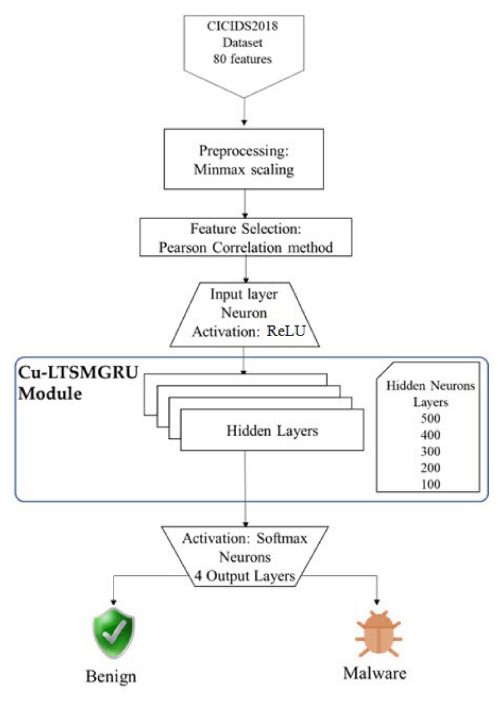
  • This system is applied to the optimum set of features of the latest CICIDS2018 dataset containing multiple types of cyber threats and attacks. This is to ensure the efficiency of the proposed IDS model in terms of accuracy and optimal complexity.
  • Massive evaluation metrics are used for an exhaustive assessment of the proposed technique, including the precision, recall, detection accuracy, F1-score, true positive rate (TPR), true negative rate (TNR), and negative predictive value (NPV).
  • The results are benchmarked with several prominent research studies to demonstrate the promising results of the proposed model.
  • Finally, the proposed approach has recorded the highest accuracy and negligible FAR compared with many current studies.
The rest of this paper is organized as follows: Section 2 provides an overview of the current IDS and related studies using different types of recurrent deep learning. The proposed approach of IDS is presented in Section 3. The system implementation and explanation of the experiments and data preprocessing are delineated in Section 4. Section 5 elaborates on the results and analysis. Finally, Section 6 concludes the work and highlights future work.

2. Related Work

Due to wide usage of cloud services, detecting attacks and malicious traffic has attracted researchers to develop a highly efficient mechanism for intrusions detection.
Researchers have developed and adopted various methods and techniques derived from deep learning. In recent years, different DL algorithms have been applied or combined to produce high-performance IDSs. Examples include auto-encoder-based IDS schemes [19,20,21], RBM-based IDS schemes [22,23], DBM-based IDSs [24,25], DNN-based IDS schemes [26,27], CNN-based IDS schemes [8,28], and LSTM-based IDS schemes [16,29]. Hybrid IDS schemes include the AE and CNN hybrid [30], the AE and DBN hybrid [31], the CNN and LSTM hybrid [32], the DNN and RNN hybrid [33], the AE and GAN hybrid [34], the AE and LSTM hybrid [35], the CNN and LSTM hybrid [36], and finally, the Variational Laplace Auto-encoder and DNN. hybrid [37].
In addition, these approaches are applied to well-known datasets, such as KDD CUP 99, NLS KDD, ISCX 2012, and CICIDS2017, and the most recent dataset, CICIDS2018.
Examples of researchers who adopted GRUs and LSTM in RNNs are as follows:
Xu et al. in [2] proposed a deep-learning-based IDS. Their model consists of four layers: a GRU, LSTM, multilayer perceptron, and SoftMax regression. The model was evaluated using two well-known datasets: KDD 99 and NSL-KDD. The achieved detection rate was 99.42% for the first dataset and 99.31% for the second dataset with false positive rates of 0.05% and 0.84%, respectively.
A machine-learning-based cooperative IDS is proposed in [1]. Among the building blocks of the deep neural network model is a denoising autoencoder. In the aforementioned study, the maximum number of hidden unites was 350. The results when applying this model to the manipulated KDD Cup 99 dataset showed that the model achieved a detection accuracy of 95%.
The IDS proposed in [4] extracted features from network data using a deep confidence neural network. Intrusion types were classified using the back propagation neural network as the top level. The KDD CUP′99 dataset was used to validate this model, and the results showed improvement over the traditional machine learning accuracy.
Riyaz and Ganapathy in [8] used conditional random fields and a linear-correlation-coefficient-based feature selection algorithm in their proposed IDS to classify features using a convolutional neural network. They reported a 98.88% accuracy using the KDD CUP′99 dataset.
Li et at. [11] proposed an IDS using a multiconvolutional neural network in which feature data were classified into four parts according to the correlation. The results showed that this model outperformed traditional machine learning and recent deep learning methods when using the NSL-KDD dataset.
The approach proposed in [38] combined both ML and DL, where both types of ML were applied: supervised learning (naive Bayes) and unsupervised learning (self-organizing maps). DL is represented by the CNN and used for feature extraction. The best DR achieved was 93%.
The authors of [39] used deep learning in their developed IDS architecture. This model was used to classify both partitioned and user-defined multiclasses. This system obtained an accuracy of 95% using the UNSW-NB15 dataset.
Tang et al. [5] proposed the gated recurrent unit recurrent neural network as an IDS for a software-defined network. The proposed model was evaluated using the NSL-KDD dataset with six features and produced an accuracy of 89%.
The IDS model developed in [10] started with a feature extraction stage. In the feature extraction process, the sequential forward selection (SFS) algorithm and decision tree (DT) model hybrid was applied. Then, a deep learning model based on both LSTM and GRUs was applied to identify two types of attacks, namely, remote-to-local (R2L) and user-to-root (U2R). The results were evaluated using the NSL-KDD 2010 and ISCX 2012 and showed an improved accuracy and detection rate over other DL models.
Few researchers have considered recent datasets, CICIDS2017 and CICIDS2018, in evaluating their DL-based IDSs. Among them, in [29], the authors implemented three DL models in their developed IDS, which are deep neural networks (DNNs), long short-term memory recurrent neural networks (LSTM-RNNs), and deep belief networks (DBNs). The system was examined using both NSL-KDD and CICIDS2017 datasets. The best accuracy for multiclass classification reported for DBN was 98.95% using the CICIDS2017 dataset and 98.77% using the NSL-KDD dataset.
Fernandez and Xu [40] applied a DNN to detect anomaly transactions in both ISCX IDS 2012 and CICIDS2017. The model was compared with other machine learning techniques, such as naive Bayes, a hybrid decision tree, and rule-based IDS and random forest. It outperformed these models since the true positive rate (TPR) was 99.93% when including the IP feature and 96.77% without using the IP address.
Choraś and Pawlicki [41] investigated different hyperparameters of artificial neural networks when applied to common datasets, NSL-KDD and CICIDS2017. These parameters include activation, optimizers, batch size, epochs, layers, and neurons. The best accuracy achieved was 99.9% when the parameter values were tanh, Adam, 100, 300, 1, and 25, respectively. However, the accuracy decreased drastically down to 5.64% for the other parameters, indicating that the ANN model is very sensitive to the parameter values.
The NIDS proposed by Chen et al. [42] was based on a convolutional neural network. The analysis was conducted on a featured dataset and raw traffic dataset extracted from CICIDS2017. The results outperformed both the support vector machine (which is a type of machine learning technique) and the deep belief network (DBN) (which is a type of deep learning technique). Their proposed approach achieved a high accuracy of 99.56% for the row dataset but 96.55% for the featured dataset.
Nayyar et al. [43] built an intrusion detection system that aimed to strike a balance between enhancing accuracy and prediction time. The model was built using an LSTM mechanism. Their system consists of three types of activation for the three layers: tanh for the LSTM layer, ReLU for the hidden layers, and sigmoid for the output layer. This model was examined using CICIDS2017, and the lowest obtained accuracy was 96.7%.
In their DL-IDS model, Bharati and Tamane [44] used a multilayer perceptron in the neural system for feed forward with a minimum of one layer between data. Their model was implemented using 100 neurons in a particular layer. The test accuracy achieved using the CICIDS2018 dataset was 95%.
The main objective of the IDS model of [45] was to detect DDoS while maintaining both speed of action and robustness against adversarial examples. The proposed model used the fast gradient sign method (FGSM) of a neural network to generate an adversarial example and to compute the gradients of a loss function with respect to the input data. The performance of the system was evaluated in terms of robustness score and recall, where the achieved recall was 98.2%.
Feature selection is one of the important stages when the data have high dimensionality. It reduces the model complexity, thus minimizing the computational cost. In addition, it simplifies the model debugging, thus enhancing the model interpretation of the learning results. Amjad et al. [13] applied the openSMILE toolkit to extract the low-level acoustic characteristics that are more suitable for the suggested speech recognition based on a deep neural network.
From the above literature of DL-based IDSs, several observations can be made. First, less importance is assigned to feature selection, since it helps reduce the complexity of the classification and identification of attacks in real time [1,2,4,7,39,40,42,43,44]. Second, although the false alarm rate (FAR) is one of the typical indicators of IDS efficiency [46], most similar works do not include it as a measure. On the other hand, those who considered it produce a high FAR [5,6,9,11,29,40,47], where the FAR ranges from 0.5% to 1.73%. Additionally, the conducted studies basically limit the evaluation to the accuracy and detection rate. Improving the accuracy, among other measures, and reducing the false discovery rate (FDR) result in reducing the workload of network experts and making the system practical and reliable for real-life implementation.

3. Methodology

The system, as depicted in Figure 1, starts by preprocessing the input data to be consistent for the later stages. In preprocessing, samples with null values are removed, textual data are converted into consistent presentation, and features are normalized. The next stage is feature selection. In this stage, the Pearson correlation method is used. The third stage is the core of the model. At this stage, the activation function ReLU is applied by the input layer to train the data. The multilayer perceptron (MLP) is also utilized at this stage to further enhance the detection accuracy. The output layer consists of four neurons with the activation function SoftMax. One of these neurons is for the benign class, and the others three are for the attack classes (FTP—BruteForce attack; SSH—BruteForce; and DoS attacks—GoldenEye).
The dataset is split randomly into an 80:20 ratio, where 80% is assigned to training and 20% is assigned to testing. The average results of 10 folds of sample data are considered to avoid bias in the results. Following splitting the data, the proposed Cu-LSTMGRU model is applied for the training process. Once the training process is completed, the trained model is utilized for the testing phase using the remaining 20%. It is used for the prediction and evaluation of performance. Details of these stages and modules are described in the following subsections:

3.1. Feature Selection

Due to the high dimensionality of the selected dataset, it is recommended to limit the number of features to reduce the training time, on the one hand [48,49], and to avoid model overfitting, on the other [50]. In addition, feature selection results in the removal of redundant and pointless features [51,52]. Feature selection plays an important role in any IDS approach. It reduces the model complexity, thus minimizing the computational cost. Further, it simplifies the model debugging, thus enhancing the model interpretation of the learning results. Additionally, it massively reduces the model training time and improves the training accuracy [49].
There are several measures for feature selection based on the correlation between features, such as Spearman’s product moment. It is also referred to as parametric statistics because it quantifies correlations on interval scales and ratios. Nonparametric statistics include the Kendall correlation coefficient, gamma correlation coefficient, and Spearman rank correlation coefficient, are another correlation coefficients [53].
For this model, the commonly used Pearson correlation formula is applied to find highly correlated features so that they can be eliminated to enhance the accuracy of the model. What features the Pearson correlation coefficient method is the dimensionless measure of the covariance of the coefficient since it ranges from −1 to 1, facilitating the interpretation, unlike the absolute value of the variance, which is difficult to interpret [54]
The Pearson correlation coefficient between two features, fi and fj, is calculated as shown in Equation (1) [55]:
P f i , f j = c o v f i , f j v a r f i × v a r f j
where cov(fi, fj) is the covariance between two features, var(fi) is the variance of fi, and var(fj) is the variance of fj. Details of calculating both covariance and variance can be found in [56].
The range of correlation coefficient values is <−1, 1>. A value of 1 means a positive correlation. A value of −1 means a negative correlation, values close to 0 represent weaker correlations, and a value of exactly 0 implies no correlation. The high correlation between features implies that these features are redundant as they carry a similar amount of information. If the feature is not relevant to other features but relevant to the output class, it is considered a good feature. Hence, highly correlated features need to be eliminated [57]. The correlation is studied based on the significance value and is also known as the p-value, which is based on the 95% confidence level. For a relationship to have a significance, the p-value should be 0.05 or less. Accordingly, 39 features are selected, and the remaining 41 features are discarded.

3.2. System Components

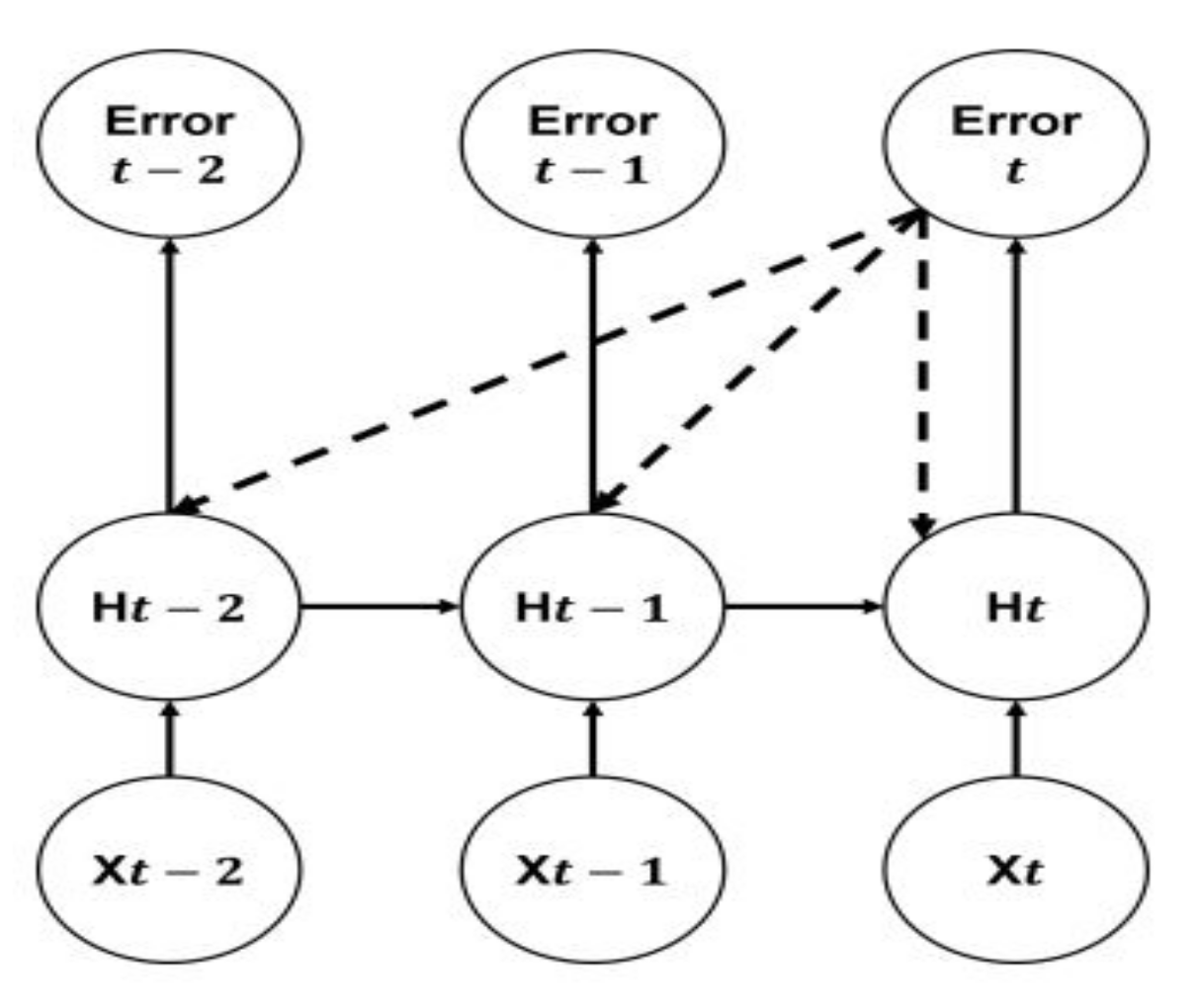
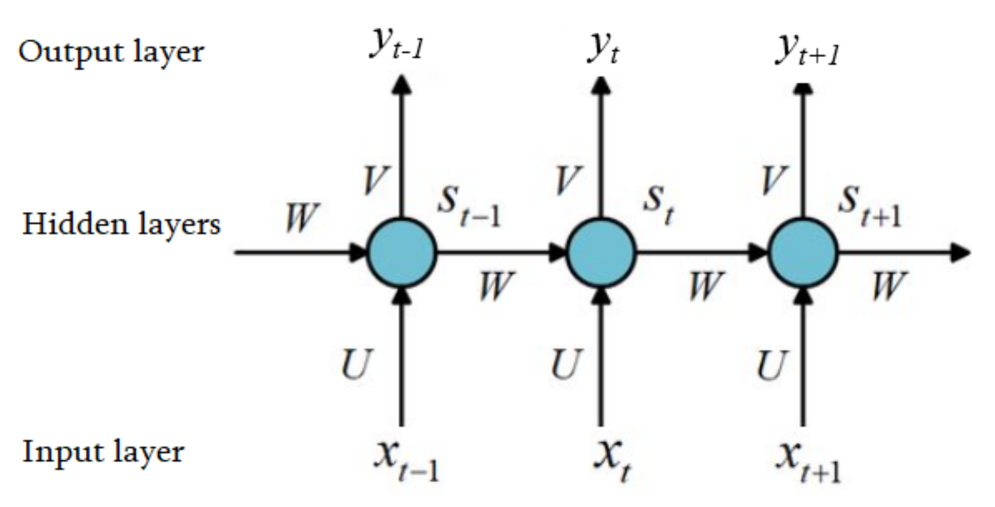
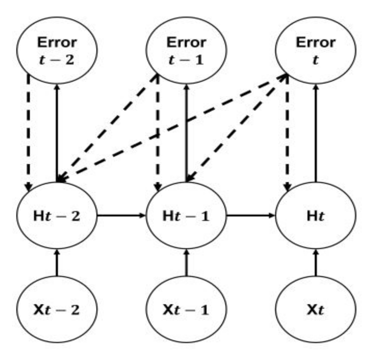
3.2.1. Recurrent Neural Network

Neurons in the same layer in a recurrent neural network (RNN) can transmit information to one another, unlike in the traditional neural network; therefore, RNN is considered superior.
RNN works according to the time sequence, thereby making it an advantageous method for performing time series tasks. Figure 2 depicts a structure diagram of the recurrent neural network.
In Figure 2, x is the input; S is the hidden state; y is the prediction result; U, V, and W are the input–hidden, hidden–output, and hidden–hidden weight matrices, respectively. Since the RNN is a time series model, the behavior and state of the network are analyzed in terms of time. Both the current input xt of the network and the previous time state St−1 determine the neuron state S at time t and are calculated as follows:
S t = F U x t 1 + W S t 1 + b h
where F is the activation function and bh is a bias term. The neuron state St is used as the output at time t and as the input of the network state at the next time t + 1 at the same time. Since St cannot be directly output as a result, it needs to be multiplied by a coefficient V, then added to the offset. This step is represented by the following mathematical formula [35]:
y t = A c t V S t + b y
where Act is the activation function and by is a bias term.

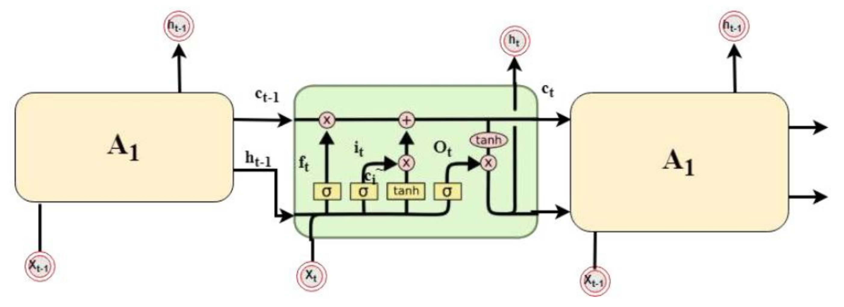
3.2.2. LSTM Neural Network

LSTM is an approach that can create a model with long-term memory, and at the same time, it can forget the unimportant information in the training data. LSTM, as depicted in Figure 3, has three differences from the classical RNN [58]:
  • LSTM has two types of activation functions: The first one is tanh, which is the most common one. Its output values range from −1 to 1. This function regulates the network data flow and avoids the exploding gradient phenomena. The t a n h function is defined as follows:
    t a n h x = e x e x e x + e x
    The second type of activation function is the sigmoid activation functions. Its output values range from −1 to 1 to allow irrelevant information to be discarded by the neural network. The sigmoid activation function is defined as follows:
    σ x = 1 1 + e x
  • Hidden state and cell state: The hidden state in the classical RNN architecture has two usages: it is used as a memory of the network and as an output of the hidden layer of the network. In addition to the hidden stats, the LSTM networks implement a cell state. The hidden state in RNN serves as a short-term working memory, while in LSTM, the cell state is used as a long-term memory to store important data from the past.
  • Gates: The values of the status in LSTM can be modified through mechanisms called gates. As shown in Figure 4, LSTM has four gates: the forget gate f, the input gate i, the cell state candidate gate c, and the output gate o. More information on these gates can be found in [53].

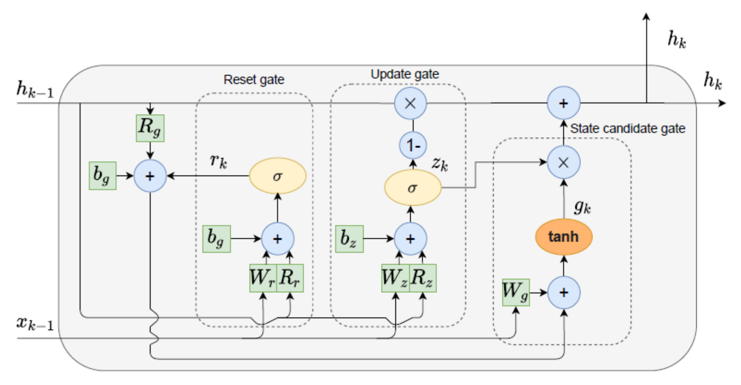
3.2.3. Gated Recurrent Unit

A GRU is derived from LSTM, with no output gate. The input gate and forget gate are combined into a single gate. Additionally, it merges the hidden state and the cell state into one state. Hence, the GRU is simpler than LSTM [16] and becomes more preferable due to its simplicity and faster training phase compared with LSTMs [8]. Figure 4 shows the architectural details of a single GRU cell [58]. The current hidden stat h(k) is calculated as follows.
If the information on a previous hidden state or the input value needs to be discarded, then the reset gate r(k) is used. The amount of information that needs to be kept and passed to the next step is controlled by the update gate z(k). The unimportant information from the previous state can be forgotten by multiplying the reset gate’s output by the previous state. In other words, if the output of the update gate z is close to zero, the current state will contain more new information. However, if the output of the update gate z is close to one, the current information is remembered from the previous time iteration.
The following calculations formulate the details explained above at the sampling time k:
r k = σ W r x k + R r h k 1 + b r
z k = σ W z x k + R z h k 1 + b z  
g k = t a n h W g x k + z k × R g h k 1 + b g
h k = 1 n N × 1 z k × g k + z k × h k 1
where r, z, g, and h are the reset gate, the update gate, the activation function, and the candidate activation, respectively. σ is the logistic sigmoid function, and × is an element-wise multiplication. W and R are learned weight matrices.

3.3. The Cu-Enabled LSTM + GRU (Cu-LTSMGRU)

The proposed framework of the IDS is composed of the LSTM and GRU, with an additional component called the computing unit, which implements two new concepts: the multipacket detection mechanism (MPDP) and many on one and many on many, as explained below.
Intrusion detection through Multipacket Detection Mechanism (MPDM): Network intrusions contain patterns corresponding to their categories. Mostly, these patterns do not occur in a packet, but spread across multiple packets. However, most of the earlier ML algorithms for IDS failed to identify these traits and do not have the capability to identify patterns that occur in multiple packets. If the identification of a DOS threat is required, this could be difficult since a DOS attack transmits numerous requests and packets, which are similar to the normal packets. This concern is not limited to DOS attacks only, but is also applicable to other kinds of attacks. Therefore, it is essential to deal with multiple packets instead of a single packet.
If we consider DOS as an example, there are several highly correlated features that contribute to forming a DOS attack. These include the source address, destination port, packet length, flow duration, timestamp, and header length. Bear in mind that the packet itself could be a normal packet, but the traffic flow style generates the attack. This flow style requires utilizing the memory elements to identify this type of attack. Each neuron at the input layer is responsible for one feature.
This proposed system will employ DL to identify whether the packet is normal or not by considering the prior packets. The prior packets and the current packets are placed in the model as an input. This could be carried out by training the model with the last label equivalent to the current packet or with all labels of previous and current packets. Consequently, the MPDM will classify the packets into abnormal or benign.
To implement this, the LSTM and GRU are featured by the memory elements, which can be used to keep the required information from the previous layer, ignore it, or combine it partially with its own input value to be passed to the next layer with specific processing according to Equations (6)–(9).
Memorizing these values and passing them to the following layers allows the better identification of this type of attack; hence, they can be propagated to the output layer through the proper classification neuron. The dense layers of the proposed model have a high number of neurons. These neurons can pass the required information horizontally (from layer to layer) or vertically (neurons within the same layer). Passing them horizontally between layers is useful for predicting related packets, which form DOS. Passing the information vertically allows the prediction of packets of a standalone attack, where the attack is not related to the prior packet to form an attack. Figure 5 illustrates this concept; the dashed lines represent the information passed horizontally from layer to layer, whereas continuous lines represent information collected vertically to classify the type of traffic.
Many on One and Many on Many: It is worth mentioning that the model can perform “many on one” kinds of classification, which classifies the current input by sequential packets, as shown in Figure 6. In this model, many inputs are given, and the output is decided only at the last step. At each time step, the model accepts a packet as input and produces a prediction output. Therefore, it is better to train the model using the previous error.
Nevertheless, it is feasible to utilize all the errors for the training; as shown in Figure 7, since the labels of the prior packets contain data that speed up the training procedure, this is called “many on many” trainings. This can identify the attack types of all prior packets simultaneously, rather than the attack type of the targeted packet alone. To achieve this concept in the present work, four additional dense layers are added before the output layer. These layers consist of 500, 400, 200, and 50 neurons. It is implemented in a way that each neuron obtains input from all neurons from the previous layer.

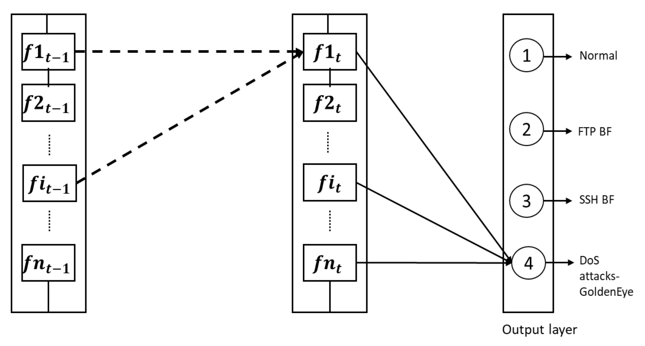
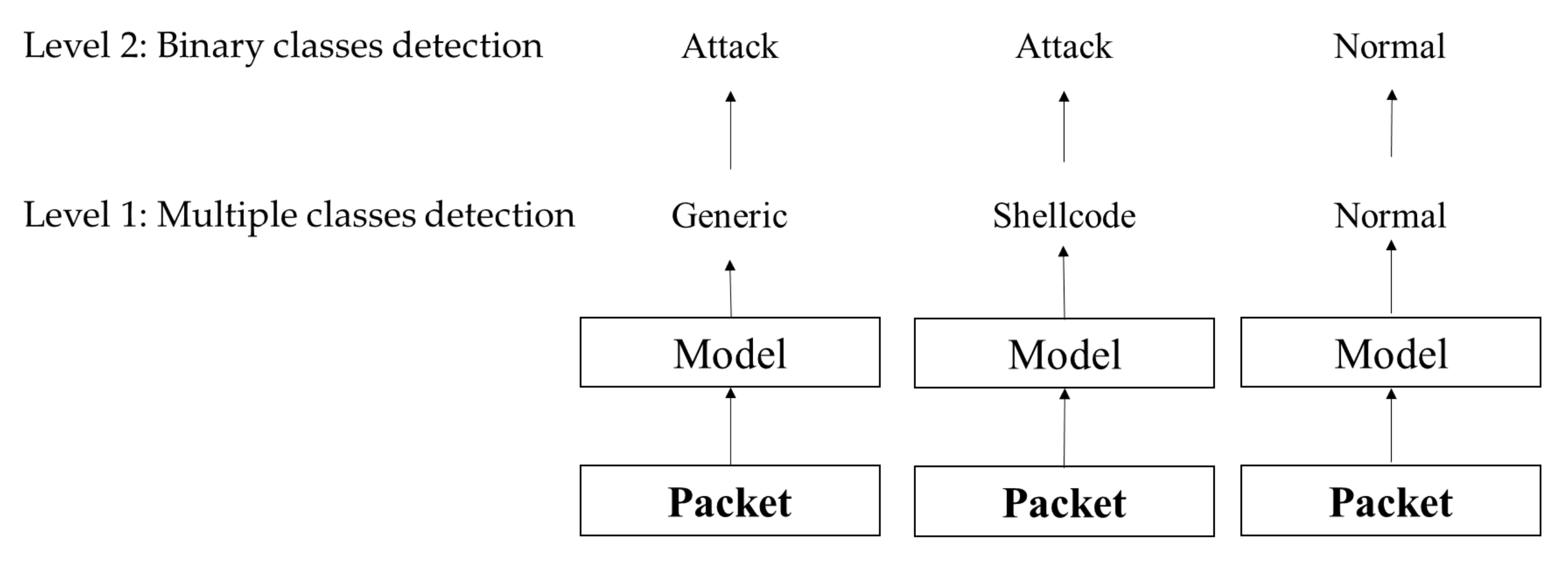
3.4. Multiple Classes and Binary Class Detection

Different types of intrusions can occur; therefore, multiclassification is needed. This is applicable when the intrusion detection system is going to react differently for each type of attack. In this case, the model is trained for different classifications, and its performance is measured using the confusion matrix of multiclass classification. The values of the true detections in this matrix are in the diagonal of the matrix, while the inaccurate detection values are in the remaining rows and columns of the matrix.
On the other hand, when all intrusions are treated equally, the different attack types of packets could be transformed into one attack type prior to the training process. Then, packets can be binary classified into abnormal or benign through model training. Otherwise, the model is trained for different classifications; then the predictions are combined into a binary classification. Performing the classification at level 1, as shown in Figure 8, represents multiple class detection, whereas performing the classification at level 2 represents binary classification (attacks or normal).

4. Implementation

The system starts by dataset preprocessing at the first stage. In the second stage, the optimal features are selected. In the third stage, three experiments are conducted to demonstrate the superiority of the proposed Cu-LTSMGRU model over LSTM and GRU.

4.1. Dataset and Preprocessing

The dataset used in this work is the one collected and prepared recently by the Canadian Institute for Cybersecurity. It was collected in 2018 and is known as CICIDS2018 [60]. The data utilized in this model were collected on 14 and 15 February 2018. These data are unbalanced since 95% of the data belong to the normal class. The sampling was performed via the Python packages SMOT (to avoid oversampling) and RandomUnderSampler (to avoid under sampling). This type of sampling was applied to avoid bias in the training dataset, which can influence the classification results.
Through the preprocessing stage, the dataset underwent two main steps: cleaning and normalization. The cleaning step consisted of several operations. First, infinite values were replaced with “nan”. Then, all records containing null and “nan” values were deleted. Next, textual values were converted into numerical values, so the data became consistent. The second step is normalization, which is a technique used to standardize the variety of features of data. The normalization here was performed through the following min–max formula:
x s = x m i n m a x m i n
This formula downscales the minimum value to 0 and the maximum value to 1. Other values are represented in decimals between 0 and 1. Therefore, Equation (10) is applied to all features in all records of the dataset as a preparation for the stage of feature selection. The preprocessing stage is shown in Algorithm 1.
Algorithm 1. Data preprocessing
1.  Begin
2.  Load data from 14 and 15 February 2018
  ## clean data
3.  Remove null values
4.  Remove infinite values
5.  Convert text into numerical format
a.  Normalize data using Equation (10)
  #Perform feature selection using Pearson correlation formula
6.  For I = 1 to N − 1 do ##N is the number of features in the dataset
a.   P f i , f i + 1 = c o v f i , f i + 1 v a r f i × v a r f i + 1
  ## Fetch the features with high correlation that represent the upper left side of the correlation matrix
7.  Relevant Features] = Correlation [Correlation > 0.9]
8.  For all features fi
9.  If fi ∉ [Relevant Features]
10.   Drop fi
11.  End For
12.  Sample_dataset = Pick 10% of the normalized dataset
13.  Sample_dataset = SMOT (Sample_dataset)      ##to avoid oversampling
14.  Sample_dataset = RandomUnderSampler (Sample_dataset) ##to avoid undersampling
15.  end
To demonstrate the superiority of the proposed model over the LSTM and GRU, three experiments were conducted, and the results were analyzed through the obtained confusion matrix as follows.

4.2. Experiment 1: LSTM Implementation and Predictions

The neurons and the layers utilized for the model-training phase were arranged in the following manner. First, the deployment of the LSTM layer with 600 neurons was performed. The second and third layers consisted of the 500 and 400 neurons, respectively; all three layers with the sequence were set to true. The fourth layer of the LSTM model was set to false because the return sequence was 100 neurons. Furthermore, the four dense layers were utilized with 400, 300, 200 and 50 neurons in a similar sequence. The activation function rectified linear unit (ReLU) was utilized for the entire layers in order not to change the volume size of each layer [8]. This function outputs the input directly if it is positive; otherwise, it outputs zero. Definite cross entropy was utilized as the loss function for the DL models.
The optimizer Adam is a procedure used to update network weights iteratively based on training data; it is preferable to other optimizers as it avoids overfitting [36]. The adoption of both ReLU and Adam is based on the extensive experiments performed by [41,58]. It was employed for the model optimization with a batch size of 32 for the reiterations of 10 epochs. Hence, the last layer of the model consisted of four neurons, one for the benign class (label 0) and three for the attack classes. The LSTM algorithm structure is shown in Table 1. Figure 9 shows that all models converge with a loss of less than 0.1 after the third epoch, and 10 epochs are enough.

4.3. Experiment 2: The GRU Implementation and Prediction

The structure of the layers and neurons utilized for the model-training phase is described as follows: The initial layer of the model contained 600 neurons. The second layer consisted of 500 neurons. The third layer was composed of 400 neurons, while the fourth layer contained 100 neurons. The employment of the first three layers with a return sequence was set as true, and the return sequence of the fourth layer was set as false. Furthermore, the four dense layers were utilized with neurons of 400, 300, 200, and 50 in the similar sequence.
The activation function ReLU was utilized for all these layers, and categorical cross entropy was utilized for the loss function (LF) of the DL models. The optimizer Adam was employed for the model optimization with a batch size of 32 for the reiterations of 10 epochs. Hence, the last layer of the model consisted of four neurons, one for the benign class and the other three for the multiclass attacks. The GRU algorithm structure is shown in Table 2.

4.4. Experiment 3: The Cu-LSTMGRU Implementation and Prediction

The structure of the layers and neurons utilized for the model training phase is as follows: All four layers of LSTMGRU with the four dense layers and a single output layer were employed. The model, GPU-enabled LSTMGRU, consisted of the following layers: The first layer consisted of 700 neurons. The second layer contained 600 neurons. The third layer contained 500 neurons, whereas the fourth layer consisted of 200 neurons. The return sequence was true for the first three layers and false for the last LSTM layer. Furthermore, four dense layers were utilized with the neurons of 500, 400, 200, and 50 in the correct sequence. The activation function ReLU was utilized for all these layers, and definite cross entropy was utilized for the loss function of the DL models.
The optimizer Adam was employed for the model optimization with a batch size of 32 for the reiterations of 10 epochs. Hence, the last layer of the model consisted of four neurons, one for the normal class and three for the prediction of the three classes of attack. The Cu-LSTMGRU algorithm structure is shown in Table 3, and the structure is shown in Figure 10.

5. Results and Analysis

This section describes two types of analysis. The first one is to benchmark the results of the proposed Cu-LSTMGRU model against the GRU and LSTM models. The second type of analysis is to benchmark the obtained results of the Cu-LSTMGRU model with the existing DL models based on similar RNN models. The comparison was performed using the common metrics used in similar studies conducted on network IDSs based on machine learning and deep learning.

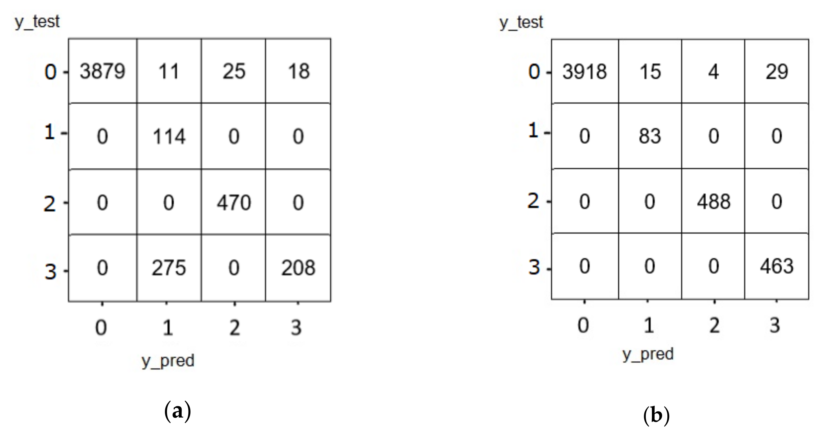
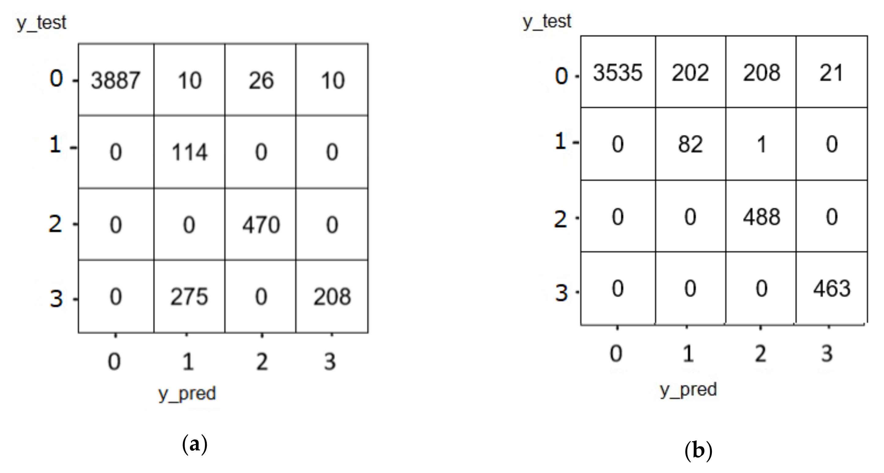
5.1. Confusion Matrices

Confusion matrix is a matrix that summarizes the performance of a classification technique where rows represent the predicted classes and columns represent the actual classes or vice versa [61].
After conducting the experiments explained in the previous section, the following results were obtained, represented as confusion matrix.

5.1.1. Confusion Matrix of LSTM

Figure 11a exhibits the confusion matrix of the results with feature selection, and Figure 11b shows those without feature selection. Labels 0, 1, 2, and 3 refer to the normal traffic, FTP—BruteForce attack, SSH—BruteForce, and DoS GoldenEye attacks, respectively. The values of the true detections are shown in the diagonal of the matrix, while the inaccurate detection values are shown in the remaining rows and columns. These figures provide an overview of the scores obtained by the model along with the types of errors made. The weighted average accuracy of LSTM with feature selection (w/FS) achieved 98%, while the accuracy without FS was 85%. It is worth noting the positive effect of using feature selection: using feature selection reduces both processing time and memory utilization. Focusing on Figure 9a, the incorrectly predicted attacks are asymmetric above and below the diagonal, where majority of the last class are classified as normal compared with seven normal records classified as DoS GoldenEye attacks. On the other hand, 664 records are classified as attacks while they are normal. Therefore, this model needs to be improved to increase the accuracy of prediction and reduce the off-diagonal errors.

5.1.2. Confusion Matrix of GRU

The classification confusion matrix of the GRU model is displayed in Figure 12. (The labels are the same as in the previous figure.) The weighted average accuracy of the GRU with feature selection (w/FS) achieved 97%, while the accuracy without FS was 99%. It is noted that off-diagonal errors are reduced compared with the LSTM model, and this complies with the expectation from the GRU model as it is an enhancement of LSTM.

5.1.3. Confusion Matrix of Cu-LSTMGRU

The confusion matrix of the Cu-LSTMGRU model presents our knowledge of the inaccuracies of the trained model and the types of the errors made, as depicted in Figure 13. The average accuracy with FS was 99.76%, while the accuracy without FS was 95%. Despite the high accuracy achieved and shown in the diagonal of the matrix in Figure 13a, the misclassification of the three types of attacks above the diagonal is very small compared with the misprediction of the third type of attack (DoS GoldenEye attacks). This classification bias may be caused by the existence of a unidirectional confusion between the categories, which could be resolved by providing more training for the model and to ensure the balance of the training and testing sets in terms of the number of records of each type of attacks to avoid such bias.
The above three experiments show the effect of feature selection on the average accuracy. Except for the GRU, the average accuracy was enhanced using feature selection for both LSTM and Cu-LSTMGRU. While its effect was higher in LSTM than in Cu-LSTMGRU, FS was improved by approximately 10% in LSTM, while in Cu-LSTMGRU, it was improved by almost 5%. In the case of the GRU, the usage of different sample sizes affected the accuracy negatively. However, the effect of no feature selection was minor in this case.

5.2. Evaluation Metrics

Several metrics could be considered to evaluate the performance, where each one reflects certain measurement criteria, such as MAE (mean absolute error), MAPE (mean absolute percentage error), SEP (standard error of prediction), REP% (relative error of prediction), RMSE (root-mean-square error), APV (average prediction variance), TSE (total squared error), and APMSE (average prediction mean squared error) [62]. However, the most popular metrics are accuracy, precision, detection rate, false positive rate, and F1-score.
Accuracy represents the proportion of the total number of records that are correctly classified by the trained model. Precision, which is also called the positive predictive value (PPV), is the number of actual attacks as a proportion of the number classified as attacks. It is used to measure how reliable the model is in classifying samples as positive. Recall, which is also called the detection rate (DR), is the number classified as attacks as a proportion of the number of actual attacks. It is used to measure the model’s ability to detect positive samples. The false positive rate (FPR) is the number classified as attacks as a proportion of the number of all normal records. The F1-score, also termed the F1-measure, is a more effective measure than accuracy. It is the balance between the precision and recall metrics to express the performance of the model. The formulas of these measures are presented in Equation (11).
A c c u r a c y = T P + T N T P + F N + F P + T N P r e c i s i o n = T P T P + F P R e c a l l D e t e c t i o n R a t e = T P T P + F N f a l s e p o s i t i v e r a t e F P R = F P F P + T N F 1 s c o r e = 2 × P r e c i s i o n × R e c a l l P r e c i s i o n + R e c a l l

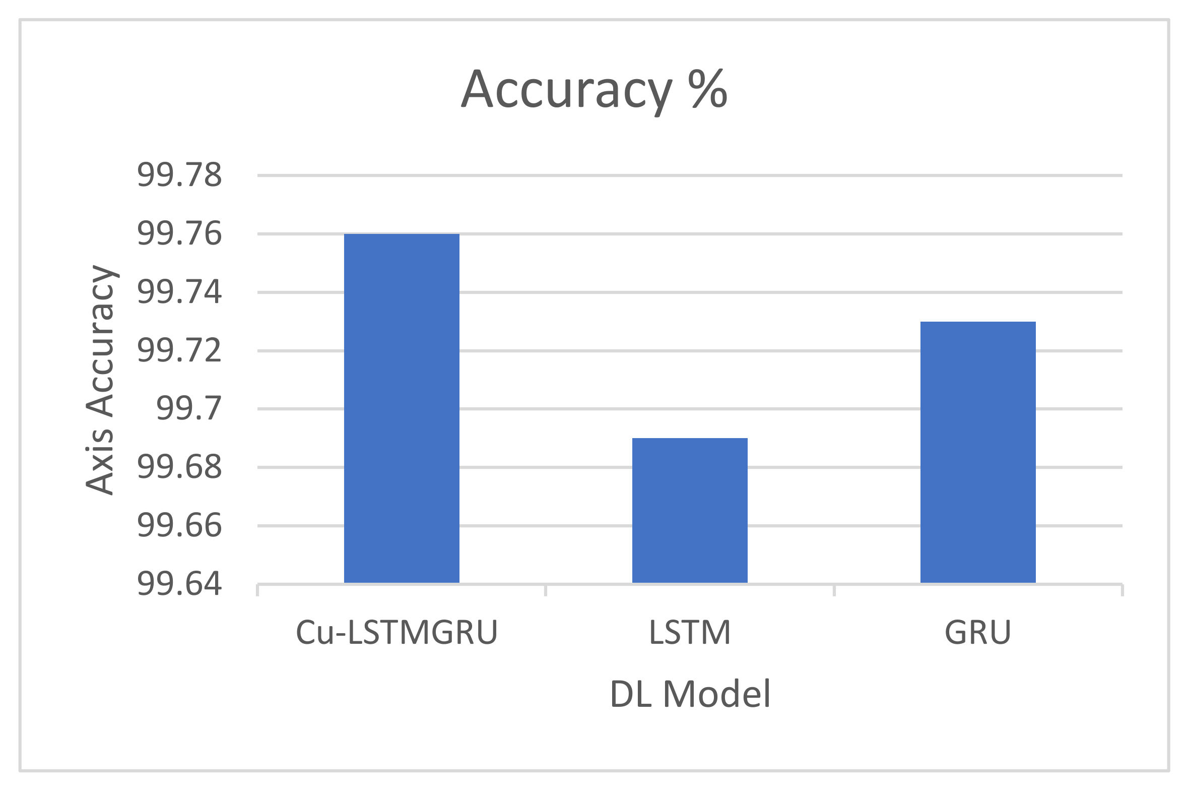
5.3. Comparison between the Proposed Cu-LSTMGRU Model, GRU, and LSTM

The first type of evaluation of the proposed GPU-enabled Cu-LSTMGRU model was compared with the two RNN models, the GRU and LSTM, in terms of accuracy. As shown in Figure 14, the Cu-LSTMGRU model achieved an accuracy of 99.76%, slightly outperforming both the LSTM (99.69%) and GRU (99.73%).
In addition to accuracy, different evaluation metrics of the system are illustrated in Figure 15, where the common metrics (TPR, precision, recall, and F1-score) are presented. The Cu-LSTMGRU model attained a high true positive rate (TPR) of approximately 86%, outperforming the other two models. Moreover, the proposed model outperformed the other two DL models by obtaining the highest precision, recall, and F1-score—98.5%, 98.5%, and 94.3%, respectively—whereas the LSTM and GRU showed a lower efficiency and attained less than 90% across all metrics except for precision of the GRU, which was 93.25%.
Furthermore, for the improved evaluation of the proposed mechanism, the assessment of the true negative rate (TNR), true positive rate (TPR), and negative predictive value (NPV) is displayed in Table 4. TNR represents the completely classified negative ratio, which demonstrates that the bigger value specifies the trained scheme with better performance. In comparison with TNR, TPR is the ratio of the completely classified positives, whereas NPV denotes the proportion of the positive and negative classification values, which eventually demonstrate the ratio between the TN and TP values.
Other metrics, including the FPR, FNR, and false discovery rate (FDR), were also analyzed for the further evaluation of the proposed model. The ratio of the inaccurately classified positive samples showed the false negative rate (FNR). The false positive rate (FPR), which is also known as the false alarm rate (FAR), describes the proportion of negative samples that have been inaccurately classified and the entire number of negative samples. The false discovery rate (FDR) measures the cause supplementation of the NPV and PPV. Their formals can simply be expressed as follows:
F N R = 1 R e c a l l A t t a c k = 1 D e t e c t i o n R a t e
FPR = 1 − Precision(Attack)
F D R = F P F P + T P
The values of the FPR, FNR, and FDR of the proposed scheme, as illustrated in Table 5, were in the range of 0.003 and 0.45, which is suitable for cloud-based attack detection in the cloud environments [63]. It is clearly noted that the FNR and FDR of the proposed model were much better than those of the other models, indicating the efficiency of the Cu-LSTMGRU model in correctly detecting the intrusion and discrimination between normal and malicious traffic.
Obviously, the proposed Cu-LSTMGRU model outperformed both the LSTM and GRU in terms of all considered measures. The experiments conducted on the optimal selected features of the CICIDS2018 dataset demonstrated the efficiency of the proposed model as a network intrusion detection system.

5.4. Benchmarking with State-of-the-Art Models

The development of network intrusion detection systems has attracted numerous researchers. The approaches vary in both the mechanisms and datasets used in the evaluation process. In particular, the benchmarking in this section was performed with those that adopt deep learning algorithms as a basis for their IDS models. In addition, the results were compared with those using the recent datasets, CICIDS2017 and CICIDS2018 (Table 4).
For the simplicity of observing the improvement of our model in terms of accuracy, the last column in Table 6 presents the improved percentage compared with each model using the same dataset. This shows that the improvement ranged from 0.16% up to 12.05%. This satisfies the objective of this work to improve the accuracy of the NIDS using an RNN-based IDS.
The model proposed by [45], which uses a convolution neural network, achieved a very similar accuracy to our model; however, the dataset used in their approach is a row dataset. When they applied the featured data, the accuracy dropped to 96.5%, and when they used a mixed dataset, the accuracy increased to 99.07%. This demonstrates the importance of feature selection, which forms one of the stages of the proposed Cu-LSTMGRU model. Another point worth noting is that models utilizing LSTM have a relatively low accuracy, ranging from 93% to 96.7%, compared with our model, which has LSTM as one component; yet its accuracy is 99.76%. This demonstrates the powerful design of Cu-LSTMGRU since it is combined with the GRU to empower its functionality.
Other measures are not fully considered by all approaches. Considering precision, for example, in [12], the lowest precision was obtained, 86.47%. However, their model performs better for other datasets, such as KF-ISAC, where the precision reaches 97%, indicating the sensitivity of the model to the dataset used. The most important achievement in the proposed Cu-LSTMGRU model is the very low FPR, which is only 0.003%. Many researchers do not consider it in their system evaluation. Having high FPR results generates a huge number of alarms, most of which are false alarms. This reduces the efficiency of the IDS. In addition, these high numbers of alarms cannot be managed by the human analyst [64].
The F1-score is another important metric used to evaluate IDSs. It is a weighted average of precision and recall. Good NIDSs should have high precision and, at the same time, high recall; however, the improvement of these two evaluation metrics is contradictory. Increasing the precision affects the recall negatively and vice versa. Therefore, the F1-score is the b average of precision and recall. According to the results presented in Table 6, few researchers consider this metric in their analysis. In [41], an F1-score of 98% is obtained as a result of the high precision and recall. A similar result is obtained in [29], which shows a precision as high as 98.86%. Nevertheless, this model lags in recall, since it is 95%; hence, the F1-score drops to 97.37%. On the other hand, the work presented in [12] has low recall (76.83%), which cannot compete with other RNN models. Hence, its F1-score is 81.36%, making it less effective. The proposed Cu-LSTMGRU model is superior to all these models. This model can report recall as high as 99.6% and a precision of 99%, producing an F1-score as high as 99.3%.
Furthermore, several researchers have implemented the GRU using different datasets. In [5], the GRU-RNN was implemented using the NSL-KDD dataset. The accuracy achieved was 89%. Although it outperforms many stat-of-the-art algorithms, it lags behind our model by more than 10%. One of the reasons for this is that the dataset has 41 features, out of which 6 are selected based on their software-defined network-related nature without any algorithm.
A similar dataset was used by Le et al. [10]. They implemented an IDS using three models, the RNN, LSTM, and GRU, separately. The accuracy was 89.6%, 92%, and 91.8%, respectively. The feature selection model was a hybrid of the decision tree and sequential forward selection models. The results of the Cu-LSTMGRU model exceeded those of this model by up to 11.3%. The results of the Cu-LSTMGRU model without feature selection were still higher than those of their model, showing the benefit of adding several dense layers.

6. Conclusions

In this work, we designed a DL-based approach for the detection of cloud computing attacks. This work employed the Cu-LSTMGRU model, which uses dense layers to develop an efficient attack detection mechanism. Experiments on the well-known recent CICIDS2018 dataset showed that the system has leading performance. Massive measures were analyzed to compare LSTM, the GRU, and the Cu-LSTMGRU model. These included the accuracy, recall, precision, F1-score, TPR, TNR, NVR, FPR, FNR, and FDR. The proposed model shows superiority over other recently published methods. We showed that the Cu-LSTMGRU outperforms other state-of-the-art algorithms with an accuracy of 99.76% and a minimal number of features using the Pearson correlation formula. This enhances the computational efficiency for real-time detection. The proposed scheme showed a very low FPR of only 0.003%. This significantly reduces the number of alarms and, hence, reduces the alarms to be managed by the human analyst, making the system practical for real-life implementation and applicable to big data in other fields.
In the future, we are interested in testing the system using different numbers of features and different mechanisms for feature selection. Other types of neural network techniques that consider both memory utilization and time complexity could be considered for further enhancement to enable a more efficient real-time detection of intrusions and attacks.

Funding

This research received no external funding.

Institutional Review Board Statement

Not applicable.

Informed Consent Statement

Not applicable.

Data Availability Statement

CSE-CIC-IDS. (2018). Datasets Research from Canadian Institute for Cybersecurity j UNB, 2018. [Online]. Available: https://www:unb:ca/cic/datasets/ids-2018:html (accessed on 5 March 2022).

Conflicts of Interest

The author declares no conflict of interest.

References

  1. Abusitta, A.; Bellaiche, M.; Dagenais, M.; Halabi, T. A deep learning approach for proactive multi-cloud cooperative intrusion detection system. Future Gener. Comput. Syst. 2019, 98, 308–318. [Google Scholar] [CrossRef]
  2. Xu, C.; Shen, J.; Du, X.; Zhang, F. An Intrusion Detection System Using a Deep Neural Network with Gated Recurrent Units. IEEE Access 2018, 6, 48697–48707. [Google Scholar] [CrossRef]
  3. Khan, M.A.; Ghazal, T.M.; Lee, S.-W.; Rehman, A. Data Fusion-Based Machine Learning Architecture for Intrusion Detection. Comput. Mater. Contin. 2021, 70, 3399–3413. [Google Scholar] [CrossRef]
  4. Peng, W.; Kong, X.; Peng, G.; Li, X.; Wang, Z. Network Intrusion Detection Based on Deep Learning. In Proceedings of the 2019 International Conference on Communications, Information System and Computer Engineering (CISCE), Haikou, China, 5–7 July 2019; pp. 431–435. [Google Scholar] [CrossRef]
  5. Tang, T.A.; Mhamdi, L.; McLernon, D.; Zaidi, S.A.R.; Ghogho, M. Deep Recurrent Neural Network for Intrusion Detection in SDN-based Networks. In Proceedings of the 2018 4th IEEE Conference on Network Softwarization and Workshops (NetSoft), Montreal, QC, Canada, 25–29 June 2018; pp. 202–206. [Google Scholar] [CrossRef]
  6. Elsherif, A. Automatic Intrusion Detection System Using Deep Recurrent Neural Network Paradigm. J. Inf. Secur. Cybercrimes Res. 2018, 1, 21–31. [Google Scholar] [CrossRef]
  7. Ambusaidi, M.A.; He, X.; Nanda, P.; Tan, Z. Building an intrusion detection system using a filter-based feature selection algorithm. IEEE Trans. Comput. 2016, 65, 2986–2998. [Google Scholar] [CrossRef]
  8. Riyaz, B.; Ganapathy, S. A deep learning approach for effective intrusion detection in wireless networks using CNN. Soft Comput. 2020, 24, 17265–17278. [Google Scholar] [CrossRef]
  9. Almiani, M.; AbuGhazleh, A.; Al-Rahayfeh, A.; Atiewi, S.; Razaque, A. Deep recurrent neural network for IoT intrusion detection system. Simul. Model. Pract. Theory 2020, 101, 102031. [Google Scholar] [CrossRef]
  10. Le, T.-T.-H.; Kim, Y.; Kim, H. Network Intrusion Detection Based on Novel Feature Selection Model and Various Recurrent Neural Networks. Appl. Sci. 2019, 9, 1392. [Google Scholar] [CrossRef] [Green Version]
  11. Li, Y.; Xu, Y.; Liu, Z.; Hou, H.; Zheng, Y.; Xin, Y.; Zhao, Y.; Cui, L. Robust detection for network intrusion of industrial IoT based on multi-CNN fusion. Measurement 2020, 154, 107450. [Google Scholar] [CrossRef]
  12. Kim, A.; Park, M.; Lee, D.H. AI-IDS: Application of Deep Learning to Real-Time Web Intrusion Detection. IEEE Access 2020, 8, 70245–70261. [Google Scholar] [CrossRef]
  13. Amjad, A.; Khan, L.; Chang, H.-T. Semi-Natural and Spontaneous Speech Recognition Using Deep Neural Networks with Hybrid Features Unification. Processes 2021, 9, 2286. [Google Scholar] [CrossRef]
  14. Phyo, P.P.; Byun, Y.-C. Hybrid Ensemble Deep Learning-Based Approach for Time Series Energy Prediction. Symmetry 2021, 13, 1942. [Google Scholar] [CrossRef]
  15. Sahlol, A.; Elaziz, M.A.; Jamal, A.T.; Damaševičius, R.; Hassan, O.F. A Novel Method for Detection of Tuberculosis in Chest Radiographs Using Artificial Ecosystem-Based Optimisation of Deep Neural Network Features. Symmetry 2020, 12, 1146. [Google Scholar] [CrossRef]
  16. Amara, N.; Zhiqui, H.; Ali, A. Cloud Computing Security Threats and Attacks with Their Mitigation Techniques. In Proceedings of the 2017 International Conference on Cyber-Enabled Distributed Computing and Knowledge Discovery (CyberC), Nanjing, China, 12–14 October 2017; pp. 244–251. [Google Scholar] [CrossRef]
  17. Maeda, S.; Kanai, A.; Tanimoto, S.; Hatashima, T.; Ohkubo, O. A Botnet Detection Method on SDN using Deep Learning. In Proceedings of the 2019 IEEE International Conference on Consumer Electronics (ICCE), Las Vegas, NV, USA, 11–13 January 2019; pp. 1–6. [Google Scholar] [CrossRef]
  18. Ashraf, N.; Ahmad, W.; Ashraf, R. A Comparative Study of Data Mining Algorithms for High Detection Rate in Intrusion Detection System. Ann. Emerg. Technol. Comput. 2018, 2, 49–57. [Google Scholar] [CrossRef]
  19. Sadaf, K.; Sultana, J. Intrusion Detection Based on Autoencoder and Isolation Forest in Fog Computing. IEEE Access 2020, 8, 167059–167068. [Google Scholar] [CrossRef]
  20. Louati, F.; Ktata, F.B. A deep learning-based multi-agent system for intrusion detection. SN Appl. Sci. 2020, 2, 675. [Google Scholar] [CrossRef] [Green Version]
  21. Mighan, S.N.; Kahani, M. A novel scalable intrusion detection system based on deep learning. Int. J. Inf. Secur. 2020, 20, 387–403. [Google Scholar] [CrossRef]
  22. Mayuranathan, M.; Murugan, M.; Dhanakoti, V. Best features based intrusion detection system by RBM model for detecting DDoS in cloud environment. J. Ambient. Intell. Humaniz. Comput. 2019, 2, 3609–3619. [Google Scholar]
  23. Masdari, M.; Khezri, H. Efficient VM migrations using forecasting techniques in cloud computing: A comprehensive review. Clust. Comput. 2020, 23, 2629–2658. [Google Scholar] [CrossRef]
  24. Yang, H.; Qin, G.; Ye, L. Combined Wireless Network Intrusion Detection Model Based on Deep Learning. IEEE Access 2019, 7, 82624–82632. [Google Scholar] [CrossRef]
  25. Wang, Z.; Zeng, Y.; Liu, Y.; Li, D. Deep Belief Network Integrating Improved Kernel-Based Extreme Learning Machine for Network Intrusion Detection. IEEE Access 2021, 9, 16062–16091. [Google Scholar] [CrossRef]
  26. Thamilarasu, G.; Chawla, S. Towards Deep-Learning-Driven Intrusion Detection for the Internet of Things. Sensors 2019, 19, 1977. [Google Scholar] [CrossRef]
  27. Zhang, J.; Li, F.; Zhang, H.; Li, R.; Li, Y. Intrusion detection system using deep learning for in-vehicle security. Ad Hoc Netw. 2019, 95, 101974. [Google Scholar] [CrossRef]
  28. Hu, Z.; Wang, L.; Qi, L.; Li, Y.; Yang, W. A Novel Wireless Network Intrusion Detection Method Based on Adaptive Synthetic Sampling and an Improved Convolutional Neural Network. IEEE Access 2020, 8, 195741–195751. [Google Scholar] [CrossRef]
  29. Elmasry, W.; Akbulut, A.; Zaim, A.H. Evolving deep learning architectures for network intrusion detection using a double PSO metaheuristic. Comput. Netw. 2020, 168, 107042. [Google Scholar] [CrossRef]
  30. Xu, X.; Li, J.; Yang, Y.; Shen, F. Towards Effective Intrusion Detection Using Log-Cosh Conditional Variational Autoencoder. IEEE Internet Things J. 2021, 8, 6187–6196. [Google Scholar] [CrossRef]
  31. Yang, L.; Li, J.; Yin, L.; Sun, Z.; Zhao, Y.; Li, Z. Real-Time Intrusion Detection in Wireless Network: A Deep Learning-Based Intelligent Mechanism. IEEE Access 2020, 8, 170128–170139. [Google Scholar] [CrossRef]
  32. Zhang, G.; Wang, X.; Li, R.; Song, Y.; He, J.; Lai, J. Network Intrusion Detection Based on Conditional Wasserstein Generative Adversarial Network and Cost-Sensitive Stacked Autoencoder. IEEE Access 2020, 8, 190431–190447. [Google Scholar] [CrossRef]
  33. Tang, T.A.; Mhamdi, L.; McLernon, D.; Zaidi, S.A.R.; Ghogho, M.; El Moussa, F. DeepIDS: Deep Learning Approach for Intrusion Detection in Software Defined Networking. Electronics 2020, 9, 1533. [Google Scholar] [CrossRef]
  34. Hara, K.; Shiomoto, K. Intrusion Detection System using Semi-Supervised Learning with Adversarial Auto-encoder. In Proceedings of the NOMS 2020-2020 IEEE/IFIP Network Operations and Management Symposium, Budapest, Hungary, 20–24 April 2020; pp. 1–8. [Google Scholar] [CrossRef]
  35. Zhang, Y.; Zhang, Y.; Zhang, N.; Xiao, M. A network intrusion detection method based on deep learning with higher accuracy. Procedia Comput. Sci. 2020, 174, 50–54. [Google Scholar] [CrossRef]
  36. Zhang, C.; Costa-P’erez, X.; Patras, P. Tiki-taka: Attacking and defending deep learning-based intrusion detection systems. In Proceedings of the 2020 ACM SIGSAC Conference on Cloud Computing Security Workshop, Virtual Event, USA, 9 November 2020; pp. 27–39. [Google Scholar]
  37. Azmin, S.; Islam, A.M.A.A. Network intrusion detection system based on conditional variational Laplace AutoEncoder. In Proceedings of the 7th International Conference on Networking, Systems and Security, Dhaka, Bangladesh, 22–24 December 2020; pp. 82–88. [Google Scholar] [CrossRef]
  38. Kumar, P.; Kumar, A.A.; Sahayakingsly, C.; Udayakumar, A. Analysis of intrusion detection in cyber attacks using DEEP learning neural networks. Peer-To-Peer Netw. Appl. 2021, 14, 2565–2584. [Google Scholar] [CrossRef]
  39. Ashiku, L.; Dagli, C. Network Intrusion Detection System using Deep Learning. Procedia Comput. Sci. 2021, 185, 239–247. [Google Scholar] [CrossRef]
  40. Fernandez, G.C.; Xu, S. A Case Study on using Deep Learning for Network Intrusion Detection. In Proceedings of the MILCOM 2019—2019 IEEE Military Communications Conference (MILCOM), Norfolk, VA, USA, 12–14 November 2019; pp. 1–6. [Google Scholar] [CrossRef]
  41. Choraś, M.; Pawlicki, M. Intrusion detection approach based on optimised artificial neural network. Neurocomputing 2021, 452, 705–715. [Google Scholar] [CrossRef]
  42. Chen, L.; Kuang, X.; Xu, A.; Suo, S.; Yang, Y. A Novel Network Intrusion Detection System Based on CNN. In Proceedings of the 2020 Eighth International Conference on Advanced Cloud and Big Data (CBD), Taiyuan, China, 5–6 December 2020; pp. 243–247. [Google Scholar] [CrossRef]
  43. Nayyar, S.; Arora, S.; Singh, M. Recurrent Neural Network Based Intrusion Detection System. In Proceedings of the 2020 International Conference on Communication and Signal Processing (ICCSP), Chennai, India, 28–30 July 2020; pp. 0136–0140. [Google Scholar] [CrossRef]
  44. Bharati, M.P.; Tamane, S. NIDS-Network Intrusion Detection System Based on Deep and Machine Learning Frameworks with CICIDS2018 using Cloud Computing. In Proceedings of the 2020 International Conference on Smart Innovations in Design, Environment, Management, Planning and Computing (ICSIDEMPC), Aurangabad, India, 30–31 October 2020; pp. 27–30. [Google Scholar] [CrossRef]
  45. Meamarian, M.; Yazdani, N. A Robust, Lightweight Deep Learning Approach for Detection and Mitigation of DDoS Attacks in SDN. In Proceedings of the 2022 27th International Computer Conference, Computer Society of Iran (CSICC), Tehran, Iran, 23–24 February 2022; pp. 1–7. [Google Scholar] [CrossRef]
  46. Pendleton, M.; Garcia-Lebron, R.; Cho, J.-H.; Xu, S. A Survey on Systems Security Metrics. ACM Comput. Surv. 2017, 49, 62. [Google Scholar] [CrossRef]
  47. Catillo, M.; Rak, M.; Villano, U. 2L-ZED-IDS: A Two-Level Anomaly Detector for Multiple Attack Classes. In Web, Artificial Intelligence and Network Applications. WAINA 2020; Advances in Intelligent Systems and Computing; Barolli, L., Amato, F., Moscato, F., Enokido, T., Takizawa, M., Eds.; Springer: Cham, Switzerland, 2020; Volume 1150. [Google Scholar] [CrossRef]
  48. Cai, J.; Luo, J.; Wang, S.; Yang, S. Feature selection in machine learning: A new perspective. Neurocomputing 2018, 300, 70–79. [Google Scholar] [CrossRef]
  49. Jaw, E.; Wang, X. Feature Selection and Ensemble-Based Intrusion Detection System: An Efficient and Comprehensive Approach. Symmetry 2021, 13, 1764. [Google Scholar] [CrossRef]
  50. Alduailij, M.; Khan, Q.W.; Tahir, M.; Sardaraz, M.; Alduailij, M.; Malik, F. Machine-Learning-Based DDoS Attack Detection Using Mutual Information and Random Forest Feature Importance Method. Symmetry 2022, 14, 1095. [Google Scholar] [CrossRef]
  51. Shakya, V.; Makwana, R.R.S. Feature selection based intrusion detection system using the combination of DBSCAN, K-Mean++ and SMO algorithms. In Proceedings of the 2017 International Conference on Trends in Electronics and Informatics (ICEI), Tirunelveli, India, 11–12 May 2017; pp. 928–932. [Google Scholar] [CrossRef]
  52. Aldallal, A.; Alisa, F. Effective Intrusion Detection System to Secure Data in Cloud Using Machine Learning. Symmetry 2021, 13, 2306. [Google Scholar] [CrossRef]
  53. Moedjahedy, J.; Setyanto, A.; Alarfaj, F.K.; Alreshoodi, M. CCrFS: Combine Correlation Features Selection for Detecting Phishing Websites Using Machine Learning. Futur. Internet 2022, 14, 229. [Google Scholar] [CrossRef]
  54. Schober, P.; Boer, C.; Schwarte, L.A. Correlation coefficients: Appropriate use and interpretation. Anesth. Analg. 2018, 126, 1763–1768. [Google Scholar] [CrossRef]
  55. Mu, Y.; Liu, X.; Wang, L. A Pearson’s correlation coefficient based decision tree and its parallel implementation. Inf. Sci. 2018, 435, 40–58. [Google Scholar] [CrossRef]
  56. Rodriguez-Lujan, I.; Huerta, R.; Elkan, C.; Cruz, C.S. Quadratic programming feature selection. J. Mach. Learn. Res. 2010, 11, 1491–1516. [Google Scholar]
  57. Biesiada, J.; Duch, W. Feature Selection for High-Dimensional Data—A Pearson Redundancy Based Filter. In Computer Recognition Systems 2; Springer: Berlin/Heidelberg, Germany, 2007; pp. 242–249. [Google Scholar] [CrossRef]
  58. Fu, Z. Computer Network Intrusion Anomaly Detection with Recurrent Neural Network. Mob. Inf. Syst. 2022, 2022, 6576023. [Google Scholar] [CrossRef]
  59. Zarzycki, K.; Ławryńczuk, M. LSTM and GRU Neural Networks as Models of Dynamical Processes Used in Predictive Control: A Comparison of Models Developed for Two Chemical Reactors. Sensors 2021, 21, 5625. [Google Scholar] [CrossRef]
  60. A Realistic Cyber Defense Dataset (CSE-CIC-IDS2018). Available online: https://registry.opendata.aws/cse-cic-ids2018/ (accessed on 25 October 2021).
  61. Barranco-Chamorro, I.; Carrillo-García, R.M. Techniques to Deal with Off-Diagonal Elements in Confusion Matrices. Mathematics 2021, 9, 3233. [Google Scholar] [CrossRef]
  62. Bolboacă, S.D.; Jäntschi, L. Sensitivity, specificity, and accuracy of predictive models on phenols toxicity. J. Comput. Sci. 2014, 5, 345–350. [Google Scholar] [CrossRef]
  63. Saljoughi, S.; Mehrvarz, M.; Mirvaziri, H. Attacks and intrusion detection in cloud computing using neural networks and particle swarm optimization algorithms. Emerg. Sci. J. 2017, 1, 179–191. [Google Scholar] [CrossRef] [Green Version]
  64. Gupta, N.; Srivastava, K.; Sharma, A. Reducing False Positive in Intrusion Detection System: A Survey. Int. J. Comput. Sci. Inf. Technol. 2016, 7, 1600–1603. [Google Scholar]
Figure 1. The architecture of the proposed Cu-LSTMGRU model.
Symmetry 14 01916 g001
Figure 2. The structure of recurrent neural networks..
Symmetry 14 01916 g002
Figure 3. The LSTM cell structure.
Symmetry 14 01916 g003
Figure 4. Gated recurrent unit structure [59].
Symmetry 14 01916 g004
Figure 5. Multipacket detection mechanism. Numbers 1 to 4 represent the different output classes.
Symmetry 14 01916 g005
Figure 6. Many on one.
Symmetry 14 01916 g006
Figure 7. Many on many.
Symmetry 14 01916 g007
Figure 8. Model with multiple packet types.
Symmetry 14 01916 g008
Figure 9. Comparison of conversion in terms of loss per epoch.
Symmetry 14 01916 g009
Figure 10. The structure of the proposed Cu-LSTMGRU model.
Symmetry 14 01916 g010
Figure 11. Confusion matrix of LSTM (a) with feature selection and (b) without feature selection.
Symmetry 14 01916 g011
Figure 12. Confusion matrix of GRU (a) with feature selection and (b) without feature selection.
Symmetry 14 01916 g012
Figure 13. Confusion matrix of Cu-LSTMGRU (a) with feature selection and (b) without feature selection.
Symmetry 14 01916 g013
Figure 14. Overall accuracy of DL models.
Symmetry 14 01916 g014
Figure 15. Comparison between DL models in terms of TPR, precision, recall, and F1-score.
Symmetry 14 01916 g015
Table 1. LSTM algorithm structure overview.
AlgorithmKernel/NeuronsLayersAFLFModel OptimizerEpochsBatch Size
LSTM
model
structure
(600, 500, 400, 100, 400, 300, 200, 50)Dense layers (9)ReLUCategorical cross entropyAdam1032
-Dropout layer
4Output layerSoftMax
AF: activation function, LF: loss function.
Table 2. GRU algorithm structure overview.
AlgorithmKernel/NeuronsLayersAFLFModel OptimizerEpochsBatch Size
GRU
model structure
(600, 500, 400, 100)GRU layers (4)ReLUCategorical cross entropyAdam1032
-Dropout layer
(400, 300, 200, 50)Dense layers (4)
4Output layerSoftMax
AF: activation function, LF: loss function.
Table 3. Cu-LSTMGRU algorithm structure overview.
AlgorithmKernel/NeuronsLayersAFLFModel OptimizerEpochsBatch Size
Cu-DNNLSTMmodel structure(700, 600, 500, 200)CuLSTM layers (4)ReLUCategorical ross entropyAdam1032
-Dropout layer
(500, 400, 200, 50)Dense layers (4)
4Output layerSoftMax
AF: activation function, LF: loss function.
Table 4. Comparison between DL models in terms of TNR, PPV, and NPV.
DL ModelsTNRPPVNPV
Cu-LSTMGRU0.99620.98300.99930
LSTM0.99540.67880.99885
GRU0.99730.93200.99885
Table 5. Comparison between DL models in terms of FPR, RNR, and FDR.
DL ModelFPRRNRFDR
Cu-LSTMGRU0.00300.14000.01695
LSTM0.00460.33190.07114
GRU0.00320.21400.06740
Table 6. Comparison of the Cu-LSTMGRU model with state-of-the-art detection mechanisms using a deep learning model.
AuthorsDatasetTechniquesAccuracyPrecisionRecall (DR)F1-ScoreFAR (FPR)Achieved Accuracy Improvement
Fernandez, 2019 [40]CICIDS2017DNN98.9---0.990.83
Chen, 2020 [42]CICIDS2017CNN99.56----0.16
Choras, 2021 [41]CICIDS2017ANN 999898--
Kim, 2020 [12]CICIDS2017CNN-LSTM9386.4776.8381.36-7.23
Nayyar, 2020 [45]CICIDS2017LSTM96.703----3.12
Elmasry, 2020 [29]CICIDS2017LSTM-RNN,
GRN-RNN,
89.09
93
99.64
99.77
87.58
92.05
93.22
95.75
1.9
2.4
0.78
Proposed ModelCICIDS2018Cu-LSTMGRU99.769999.699.30.003-
Catillo, 2020 [47]CICIDS2018Two-level deep learning98.2596.998.63-1.081.50
Meamarian, 2022 [44]CICIDS2018FGSM of a neural network--98---
Bharati, 2020 [43]CICIDS2018Multilayer perceptron (MLP)95----4.97
Xu, 2018 [2]KDD Cup 99BGRU + MLP + SoftMax99.84 99.42 0.5−0.12
Tang, 2018 [5]NSL-KDDGRU-RNN89 12.05
Le, 2019 [10]NSL-KDDRNN89.6 11.30
LSTM92 8.39
GRU91.8 8.63
Fu, 2022 [58]IADA, IADBBiLSTM-DNN 97.293.995.8
Publisher’s Note: MDPI stays neutral with regard to jurisdictional claims in published maps and institutional affiliations.

