Abstract
We review the problem of summation for a very short truncation of a power series by means of special resummation techniques inspired by the field-theoretical renormalization group. Effective viscosity (EV) of active and passive suspensions is studied by means of a special algebraic renormalization approach applied to the first and second-order expansions in volume fractions of particles. EV of the 2D and 3D passive suspensions is analysed by means of various self-similar approximants such as iterated roots, exponential approximants, super-exponential approximants and root approximants. General formulae for all concentrations are derived. A brief introduction to the rheology of micro-swimmers is given. Microscopic expressions for the intrinsic viscosity of the active system of puller-like microswimmers are obtained. Special attention is given to the problem of the calculation of the critical indices and amplitudes of the EV and to the sedimentation rate in the vicinity of known critical points. Critical indices are calculated from the short truncation by means of minimal difference and minimal derivative conditions on the fixed points imposed directly on the critical properties. Accurate expressions are presented for the non-local diffusion coefficient of a simple liquid in the vicinity of a critical point. Extensions and corrections to the celebrated Kawasaki formula are discussed. We also discuss the effective conductivity for the classical analog of graphene and calculate the effective critical index for superconductivity dependent on the concentration of vacancies. Finally, we discuss the effective conductivity of a random 3D composite and calculate the superconductivity critical index of a random 3D composite.
1. Introduction
Real physical systems can almost never be studied in terms of exact solutions to their governing dynamics. However, it is often possible to find asymptotic expansions of solutions in the vicinity of some characteristics to the problem boundary points. The ultimate goal is to construct a good approximation for the sought function, representing the solution to the problem, valid on the whole domain of its variable(s), having as an input only its asymptotic behavior near the boundaries. A typical complication is associated with availability most often, only of a few terms of the asymptotic expansions.
Sometimes, we have to derive asymptotic power laws that are ubiquitous in nature. Sometimes, following Feynman, one would attempt to estimate in a given order the result for the expansion coefficient(s) without the brute force evaluation. Sometimes the general structure of the expansion can only be guessed. Many instances of such problems were discussed in the books [1,2,3,4]. Most recently, the disordered hyperuniform composites were reviewed in [5].
The transport coefficients in random and regular media could be expressed as expansions in a concentration of particles f. Despite persistent efforts of such outstanding researchers as Einstein, Batchelor, Brady, Jeffrey, Milton, McPhedran, Torquato, Wajnryb and Mityushev, most recently, the problem still exists of finding long enough and correct expansions. When it is only possible to find short truncated series, their true value may still need clarification. Such expansions are relevant for small f.
The transport coefficients such as effective viscosity, permeability, sedimentation rate, elastic moduli, effective diffusion coefficients and conductivity behave critically when approaching critical points in concentration. The relation between the two types of expressions is difficult to establish. However, it has to be looked for if the ultimate goal of a complete understanding of the whole region of concentrations is to be achieved.
The problems of finding critical indices for the effective transport properties are decidedly non-universal, meaning that there is no simple formula and (or) explanation of the value. This is in sharp contrast with the theory of critical phenomena in thermodynamics, where the critical indices are universal [6], meaning that the formulas exist, covering different physical systems and explaining the indices in terms of spatial dimension and number of components of the order parameter. Thus, for transport properties, the challenge consists in developing the solution in each and every case separately, almost from scratch, when existing methods fail.
However, certain universality exists in the methodology. In all cases, we have a short expansion in concentration f of particles (or close in meaning) for small f. On the other side of high concentrations (or equivalent), we are aware of the power-law behavior. In some cases, the critical properties have to be calculated from the expansions on the other end. In some cases, the two asymptotic tails are known, and we have to merge them into a single formula. The location of criticality is also known from geometrical considerations most often, or the power-laws can be attributed to infinity. Another common salient feature is the shortness of the expansions and ensuing paucity of coefficients in the expansions.
To approach the problem, we had to master or even develop some special tools for the two closely related problems, such as
- (1)
- The derivation of critical properties, such as indices and amplitudes from the short truncated versions of the putative complete expansions for the effective quantities, or critical problems;
- (2)
- Approximation methods for deriving formulas from the sought quantities from their known asymptotic expressions, or crossover problems.
Thus, the main goal is to attack the group of problems, including critical behavior of the effective transport properties and develop special methods for their solution. All the systems and critical problems considered in the review are being studied extensively and are important on their own merits. However, putting them together and analyzing them by similar methods is intended to stress their commonality. Of course, the commonality is due to the interactions between inclusions taken into account in low orders, as well as criticality arising at some common geometrical threshold.
In Section 2 and Section 3, we discuss the effective viscosity (EV) of random, active and passive suspensions by means of a special algebraic renormalization approach. It is applied to the first and second-order expansions in volume fractions of particles suggested by Einstein, Batchelor et al. The EV of the two-dimensional and three-dimensional passive suspensions is analyzed by means of various self-similar approximants.
A brief introduction to the rheology of micro-swimmers is given. Microscopic expressions for the intrinsic viscosity for the active system of puller-like micro-swimmers are obtained. It turned out that the methods developed for passive suspensions could be applied to the active system of the pullers. For active systems, we have to actually solve the two crossover problems in a row. The first is with respect to their activity, and the second of interpolation between the two concentration regimes.
In Section 4, special attention is given to the problem of calculation of the critical indices and amplitudes of the shear modulus of random elastic composites.
In Section 5, we consider the sedimentation problem and discuss the sedimentation rate in the vicinity of critical points. Critical indices are calculated from the short truncation by means of minimal difference and minimal derivative conditions imposed directly on the critical properties.
In Section 6, crossover expressions are presented for the non-local diffusion coefficient of a simple liquid (another random system) in the vicinity of a critical point, dependent on the wave-number of density fluctuations in the liquids. Extensions and corrections to the celebrated Kawasaki formula are discussed.
In Section 7, we discuss the effective conductivity for the classical analog of graphene with the random addition of vacancies and calculate the effective critical index for superconductivity dependent on the concentration of vacancies.
Finally, in Section 8, we discuss the effective conductivity of a random 3D composite with perfectly conducting spherical inclusions and calculate the superconductivity critical index of such a random 3D composite.
Methods required in the course of the analysis are discussed when necessary and to the extent required. Relevant references are always given for more details to be learned. Since no one can cover the immense subject in its completeness, the presentation will be anchored to the topics most familiar to the author. Only a few problems of transport coefficients where short truncations are known for quite some time or were obtained only recently, were analyzed in regard to their critical properties or crossover behavior. However, they are all of significant interest in the theory of composites, suspensions and simple liquids. New methods developed for critical and crossover phenomena bring new insights to the effective transport coefficients.
The four effective transport coefficients, such as effective viscosity, sedimentation rate, elastic modulus and effective conductivity, are the most popular in the field of effective properties of composite media and suspensions. A similar problem of non-local diffusion coefficients is one of the central points for research in the theory of simple liquids.
However, there are some other important problems, including criticality in various contexts. Permeability in wavy channels also behaves critically or demonstrates a power-law behavior. Several examples of the effective permeability in wavy channels can be found in [7]. The rather long truncated series is given in terms of waviness [4]. Their analysis is more traditional since one can observe a good numerical convergence for the critical indices and amplitudes for the effective permeability. Striking power-laws were also discovered in the gap sensitivity in optimized photonic crystal and disordered networks as the function of the dielectric contrast [8]. The diffusion process in complex media is found to exhibit different regimes, including power-laws, dependent on the length scale [9].
2. Viscosity of Passive Suspensions
Keep in mind that in isotropic Newtonian fluid viscosity, is a scalar quantifying the rheology of the fluid, establishing the relation between the macroscopic strain-rate and stress in the fluid. The effective interactions among the colloidal particles in suspensions are described almost perfectly by the hard-spheres model. The phase behavior of hard spheres includes liquid, crystal, and metastable states, with associated phase transitions and crossover.
Thus, hard-sphere fluid is the simplest and most widely used reference model for describing the behavior of real fluids and concentrated colloidal suspensions. The particles (colloids) can be viewed as large atoms. There is an understanding that the hard spheres equation of state, as well as various effective transport properties, may be extended smoothly, avoiding the first-order freezing transition to describe the metastable fluid branch. In the most interesting three-dimensional case, the metastable branch ends at its first singularity at a random close packing (RCP) volume fraction [4,10].
The fundamental idea of Einstein (1906) was to quantitatively express the notion that the viscous energy dissipation rate of the suspension must be equal to the dissipation rate of the effective homogeneous fluid. Such a condition leads to the definition of the effective viscosity applicable for any volume fractions up to the threshold where lubrication forces dominate [11]. Such an approach naturally includes both passive and active suspensions of cells and bacteria considered in the subsequent Section 2 and Section 3. The effective viscosity could be measured experimentally and may become negative in open bacterial systems as well [12].
While our main interest is in the most physically and biologically relevant case of three-dimensional (3D) suspensions, models of two-dimensional (2D) suspensions can serve as important additional tests of our method. Furthermore, understanding the rheological properties of 2D suspensions may carry considerable importance for the understanding of the function of lung surfactant monolayers, even in developing possible treatments, since the divergent surface viscosity plays a crucial role in breathing [13,14].
Since both two-dimensional and three-dimensional contributions to the viscosity are present for thin films [15], the importance of studying idealized 2D systems is apparent. Thus, we first review the case of the 2D suspensions of impenetrable hard disks immersed in a fluid of viscosity .
2.1. Effective Viscosity of 2D Passive Suspensions
The effective viscosity problem can be approached as a peculiar critical phenomenon. The expansion of effective viscosity in the volume fraction of hard disks , where r is the disks radius and n is the number density of particles, is available theoretically only up to the first-order term as [16,17],
where is the viscosity of the solvent. Clearly, such truncation is not sufficient to develop any meaningful and consistent approach to high-volume fractions. We have to recognize that, in addition, there is a critical point characterized by a power-law divergence of the viscosity in the vicinity of the maximum volume fraction value ,
The value of the critical exponent for viscosity has not been explained theoretically but is known experimentally [18,19]. The value of critical amplitude A has to be estimated in the course of calculations. From simulations with soft disks in two dimensions, using a bi-disperse mixture with equal numbers of disks of two different radii, it is found that [20].
In our approach to the derivation of the analytical expressions for the effective viscosity of 2D suspensions, we are going to employ the renormalization group (RG)-inspired technique of [21]. The next component of our approach in our manipulations is to dwell on the intuition of the great scientists. Feynman thought to avoid tedious calculations if possible and replace them with rather simple but direct estimates for the coefficients in the perturbative theories.
A couple of analytical expressions for the effective viscosity have been developed over the years. Here, we include several that we find the most useful for comparison with the results derived in this paper. The most often used is the well-known Krieger–Dougherty (KD) equation, applicable in 2D as well as in 3D.
This is a crossover expression that links polynomial and power–law behaviors at opposite ends of the concentration interval. It can be written explicitly as
so that one can note that the critical exponent from (3) is much larger than but is more compatible with [20].
As the benchmark, we will also use the 2D variant of the simple crossover equation suggested in [11]
where . From (4), one can evaluate the second-order coefficient in the expansion , as well as the critical amplitude .
The main shortcoming of the renormalization group method employed in [22] is that the authors only use a perturbative theory for small f and exclude critical point behavior. Below, we specialize the formulae to
with the critical index denoted by . By definition, in the vicinity of the critical point, has the following asymptotic behavior as
where A is the critical amplitude.
The critical exponent is the limit of the effective critical exponent defined in a neighborhood of :
Let us note that with help of the Euler transformation,
the critical behavior can always be moved to infinity.
If we define a new quantity then
On the other end of the interval at small x the function has a polynomial truncation, with the k-th order approximant given by the series
with integer . In the k-th order effective exponent can be defined here analogously by
which, for , has an explicit expression valid for small x,
One would strive to extend to the whole interval . To such an end, one can derive a self-similar approximation [21,23], for the effective critical exponent . It should also be taken into account that
The value of may be assumed to be known in advance, and its value is finite. However, it can be calculated as well from the expansion at small x.
Finally, from the knowledge of one can approximate the sought function, , by integrating (6), obtaining
The critical amplitude A can be evaluated from (12) as
The formal method of self-similar approximants may, in general, lead to multiple solutions to and, hence, to . Indeed, the formally constructed fixed point depends on unknown exponents and amplitudes, which parametrizes the most general expression for . With sufficiently many terms in the perturbative expansion, it may be possible to determine the parameters uniquely by selecting them so that all the , as well as the critical threshold and exponent, are reproduced. When only low-order expansions are at our disposal, as is frequently the case, additional choices have to be made to select appropriate parameter values for self-similar approximants.
The most frequently used here are what we refer to below as the root, iterated root, factor, and super-exponential approximants [3,4]. Some precise definitions of the relevant constructions will be given a bit later in Section 2.1.1. For convenience, most important notions will be collected in the Nomenclature section. However, we think that for many simpler cases have been discussed in the first order of perturbation theory, and even in the more advanced second-order, emerging formulas are transparent enough and are self-explanatory. In our opinion, a clever researcher could have guessed them if needed.
It is important to be able to make the extrapolation by several methods and then compare the results. If these results yield close values, this suggests that the extrapolation (or interpolation) is reliable.
In line with this idea, we employ the self-similar approximants within the single framework and strive to show that they are close to each other. The latter observation would indicate that the basic approach is robust and not overly sensitive to the uncertainty arising from working with small-concentration expansions or incomplete knowledge of the critical point.
We refer to our own results as obtained by the Algebraic renormalization method (ARM). ARM dwells on studying and drawing conclusions from various expressions for the effective critical index (-function) in the lowest orders of perturbation theory.
Using a change in variables and the simplest root approximant [24], one can obtain the simplest expression for the effective critical index from the first-order perturbative expansion:
where
This is a linear expression, which after integration of (12) with yields the following formula
Asymptotically close to the critical point, we recover a power-law, while at small concentrations, the exponential term dominates. The second-order coefficient and the critical amplitude are easily evaluated from (15) and found to be
One can also look for the solution in the form of an iterated root. Iterated roots of the type
were designed to find all the parameters iteratively (see [25] and Section 2.1.1 for a complete definition of iterated roots) in such a way that
so that
The result of integration can be expressed in closed form by means of a simple formula
where . The intermediate expressions occurring in the course of integration are not shown here. They are rather cumbersome [21], but the simple formula can be established through the direct comparison of the expansions in arbitrary order. From the expression (19), we easily analytically evaluate
again, larger than what follows from (4).
However, one can also try to approximate the effective index by the following simple exponential approximant [26],
where is obtained from the condition .
In this case, the effective viscosity can be written using an exponential integral
so that
Directly, one can obtain the second-order coefficient in the expansion and the amplitude. It equals
Let us also try to estimate the third-order coefficient, assuming that , the value chosen between the three estimates for the second-order coefficient just derived above. Note that one is not obliged to include the trivial zero-order term into the resummation directly, but simply can leave it outside and just re-use the results of ARM. Then, there are two simple expressions for EV, which respect one exact and one calculated coefficient,
It generates the third-order coefficient in the expansion and the critical amplitude
Based on the same idea, the second expression of such type can be readily written down,
It generates the corresponding third-order coefficient in the expansion and the critical amplitude
In the above expressions, unknown coefficients and are found from asymptotic equivalence with the truncated expansions.
Finally, using the third suggested form of the -function (20), we find after the same shift yet another expression in terms of the incomplete gamma function,
Formula (24) produces the third-order coefficient in the expansion and the critical amplitude
All of our above solutions work well compared with the numerical data up to . For example, at , (15) predicts the EV of against numerical , with similar accuracy for smaller f. However, one should take into account that it is a much smaller value for maximum volume fraction used in computations of [27], which are available up to . The numerical agreement is expected to become better when the higher threshold is used.
Another convenient expression for the effective viscosity can be suggested by directly applying the factor approximant,
with the third-order expansion coefficient and the critical amplitude
appearing close to the other estimates. In general form, the factor approximants will be presented a bit later in the (34). However, it is quite straightforward to observe that formula (25) is a multiple of two factors, each of them being the simplest root-form [3,23].
Thus, in the 2D passive case, we suggest, for instance, formula (23) for the whole range of concentrations. The predictions of the formula are in good agreement with the results of direct numerical simulation [27]. We also estimated the second-order expansion coefficient, the third-order expansion coefficient and the critical amplitude,
In comparison, in [28], a slightly larger result for the second-order coefficient is obtained. It was found that by extrapolation from the confined geometry for athermal disks. Such a difference in with our estimates is to be expected since, in our study, we do not specify the strength of thermal fluctuations but draw additional information from high-concentration limits, where thermal and athermal cases look very similar.
To check the consistency of such estimated values for , let us try to estimate the critical index along the different route, as suggested in [29,30]. Assume also that in the vicinity of a threshold,
with unity to be expected as the usual contribution from the radial distribution function at the particle’s contact , [29,30], and the value of coming from the hydrodynamic interactions in the suspension. With the total value of the critical index , we expect that . One can suggest, for the effective viscosity, a simple root approximant
which, by design, takes the unity contribution into account. After imposing the asymptotic equivalence with the polynomial
in the third-order, we find
with an estimated value for , reasonably close to expected. The amplitude could be estimated from (26) as well, bringing .
2.1.1. Comment on Critical Index and Diff-Log Borel Summation
Consider the case when has the following asymptotic behavior as
Furthermore, let the critical index be known in advance. One can also calculate the critical amplitudes using the method of self-similar Borel summation introduced in [31]. Mind that the problem of critical behavior with a finite threshold (2) can always be mapped to the problem (27) by applying Euler transformation (7), or similar, as in (57).
The Borel summation method could be devised through the Borel transform,
The intention here is to simplify the problem by removing the superficial factorial growth of the coefficients . Working on the transformed series with some other approximants may bring about more accurate results. However, returning to the original problem is not so easy. To perform an inverse transformation, one should compute the integral numerically. However, recently, some progress was achieved in [31,32], allowing us to find analytical expressions for the critical amplitude A and index . In the case of the Borel summation, one can easily avoid numerics and use only formulas. Calculations are particularly easy to perform with the iterated root approximants.
Summing up the truncated series by means of iterated self-similar root approximants [3,4,32] yields the approximant
The inverse Borel transformation
gives the approximation for the sought function . At large values of x, function (30) is expressed as follows,
where the critical amplitude
The marginal amplitude
follows from the definition of iterated root.
One can also apply for the purpose of the Borel summation the self-similar factor approximants [3,4] in the form
where
The condition on the exponent
should be respected as well. For the factor approximants, marginal amplitude for the transformed series is given by the expression
Calculations could be performed with relative ease using formulas, strictly following the structure of the example presented in (Section 7, [31]). To the Borel-transformed series, we apply factor or iterated root approximants and simply find the leading term at infinity, behaving as a power law. The power calculated in such a manner is nothing else but the sought critical index [31].
As for the amplitude, it consists of the critical amplitude of the factor approximants applied to the transformed series, scaled by a Gamma-function appearing in the course of inverse transformation and dependent only on the found critical index [31]. Thus we find , .
With the value of the critical index fixed to and factor approximants given by (34), we can recalculate by using the same method of self-similar Borel summation [31]. If, instead of a factor approximants, we employ iterated roots, the result remains quite close, i.e. . In both situations, we observed reasonably good numerical convergence to the quoted numbers.
Critical indices can also be found by using the techniques developed for critical amplitudes. Let us deal now with a function with power-law asymptotic behavior
The critical exponent can be expressed as a diff-log function of the limit
where as shown, e.g., in the books [3,4].
When the small-variable expansion for the original function is given by the sum , we can find the small-variable expression for the diff-log function ,
which can be expanded in powers of x, leading to the truncated series
However, for , we find that simply
where the “ critical amplitude” is the sought critical index , and the “critical index” is fixed to to make the limit (37). We can also apply the technique of iterated roots described above for the critical amplitudes and calculate the critical index . Then, it remains to simply apply the methods to be developed to calculate also the critical index . However, the case of , appears to be divergent, or indeterminate, when treated by the self-similar Borel summation technique of [31]. In such cases, some other types of summation could be used, similarly to in the paper [32]. Such summations, called Borel–Leroy and Mittag–Leffler summations, include some control parameters [32]. The parameters could be found from the minimal-difference, or minimal derivative conditions imposed on critical amplitudes [4].
There is also some simple way to avoid divergence. Let us consider an inverse,
With such a critical index, there is no divergence in the formulas of [31]. Now the value of critical amplitude can be found following [31]. After resummation, say with iterated roots [32], we will arrive at the resummed amplitude and
where gives the sought value of the critical index .
The technique just discussed can be readily applied to the case of critical index . The first-order iterated root properly conditioned at infinity gives , while in the second-order . Application of the second-order factor approximant leads to the estimate very close to the latter value.
Both methods of Borel summation [31,32], also explained in Section 2.1.1, especially with iterated roots, are very easy to work with since the computations are performed on explicitly given formulas.
2.1.2. Comment on Critical Index and Elasticity-Viscosity Analogy
Consider special 2D composite material with an incompressible matrix and perfectly rigid, incompressible inclusions. It represents an elastic analog of the viscous suspension [4].
The snapshot of a random media studied below is displayed in the book [4]. Lengthy but straightforward Monte-Carlo computations result in the polynomial formula for the effective viscosity of 2D random suspension valid for small f,
The elasticity-viscosity analogy, in principle, allows us to take into account all elastic & hydrodynamic interactions between inclusions and map them into effective interactions of the pairs, triplets, etc. of groups of the inclusions. Of course, there is no trace of a Brownian motion in such an approach. On the other hand, less sophisticated estimates by ARM presented in the main body of the section allows us to potentially take them into account indirectly.
Application of the self-similar Borel summation with factor approximants from Section 2.1.1, generates single real, non-trivial estimates in the third-order of the perturbation theory, . The higher-order estimates produce only non-physical, complex solutions. Application of the diff-log Borel summation with iterated roots and inverse transformation discussed in Section 2.1.1 brings again only a single non-trivial estimate in, de-facto, the same order, . Again, only complex results are generated in higher orders.
Let us employ the Euler transformation (7),
In terms of the transformed variable, let us construct the iterated root approximants introduced in Section 2.1.1,
and define the parameters from the asymptotic equivalence with the original truncated series for the effective viscosity. This gives the large-z asymptotic form
where the amplitudes are
In order to calculate the critical index , we analyze the differences for the critical amplitudes in k-th order, as prescribed in [4,33],
The control parameters are defined as the solution to the minimization problem
The results of calculations are presented in Table 1. As shown in [4], the most reasonable estimate for the index equals ,

Table 1.
Critical indices for the viscosity obtained from optimization conditions on .
The latter value for the index appears to be compatible with the experimentally found number , quoted in the book [1], justified by the elasticity-viscosity analogy [4]. It is smaller than the otherwise measured value of since only an elastic (hydrodynamic) contribution to the index is considered. Currently, we are not aware of the consistent estimates for the contributions from the 2D Brownian motion, unlike in the 3D case to be discussed in what follows.
2.2. 3D Viscous Suspensions
We now apply the ARM method to the case of passive suspensions of spherical particles. The effective viscosity of random suspensions of the hard spheres with the stick boundary condition is always of great interest, as the researchers strive for a long time to obtain an accurate and compact formula for arbitrary concentrations. The expansion in the volume fraction of hard spheres , where r is the spheres radius and n is the number density, is available up to the second-order term as :
and for non-interacting hard spheres, the result is due to Einstein (1906).
Finding the second-order coefficient turned out to be a great challenge. Batchelor [34] found that , and Wajnryb and Dahler [35] obtained . The result for takes into account the two different mechanisms. It consists of the hydrodynamic contribution , with the addition of the smaller contribution from the Brownian motion of the order of unity. We tend to use Batchelor’s estimate. However, we will also recall the Wajnryb and Dahler estimate when required. The effective shear viscosity behaves critically,
The threshold here corresponds to the random closest packing of hard spheres at . The value of the critical exponent for the viscosity in 3D, can be satisfactorily deduced both theoretically and experimentally [19,29].
For practical purposes, for three-dimensional situations, even with varying threshold values and model assumptions, it was suggested to consider such divergence as a universal power-law with the value of [36].
2.2.1. First-Order Interpolation
Thus, near the critical point, the EV in the 3D case has a divergent behavior (45), with . At the other end of the interval for small f, it is expressed as the second-order polynomial. Let us proceed similarly to the 2D case studied above and in accordance with the paper [21], where more technical details could be looked up. Our primary target is a subsequent application to the case of active suspensions in Section 3 since in that case, only first-order information is available.
In addition to , we are now able to construct in the next Section 2.2.2. For and small x, we have an explicit expression (10),
In terms of the variables , one can easily obtain the simplest expression for the effective viscosity [24],
One can also look for the -function in the form of an iterated root
where
After integration in (12) with , we arrive, after some transformations, at the surprisingly simple explicit solution:
Another way to approach the problem is simply to approximate the effective index by the exponential approximant [26],
where the control parameter has to be obtained from the condition
In this case, integral (12) can be written in the general form
Directly from the expressions (46), (48), (50), one can plausibly estimate the second-order coefficient in the expansion. It equals, respectively,
2.2.2. Second-Order Interpolation
Let us now consider the second-order approximation to the effective critical index,
Transformation of the independent variable. In the paper [21], the following expression for the effective critical index in the form of a second-order iterated root [25],
was suggested. The parameters should follow from the asymptotic equivalence in the region of small f as well as from the critical regime. In general form, iterated roots are given by formula (40). Numerical analysis of the integral (12) for effective viscosity allows us to find the critical amplitude,
Iterated Root. However, another expression was suggested in [21]
utilizing the higher-order iterated root [25]. Imposing the condition on critical points together with usual asymptotic conditions, one can obtain all parameters in (53) explicitly. Again, the EV is given numerically by the integral (12). One can also find the corresponding critical amplitude,
Super-exponential and root approximants. One can also construct the so-called super-exponential approximant [26],
as shown in [21]. The parameters can be found in [21]. After numerical integration (12), one can find
Similarly, but using a root approximant [3,24]
with
after integration (12), one can then find the critical amplitude
Averaged approximants. A different approach to the second-order problem could be based on pairwise weighted averages of the expressions obtained in the first-order, such as (46), (48), (50). In total, three such pairs are available. For example,
The weight is determined through the asymptotic condition on the second-order coefficient . By analogy, one obtains and . Averaged approximants will be employed in Section 3.
2.2.3. Factor Approximants and Estimates for the Critical Index
As explained in the paper [21], one can take into account some additional proposition on the expansion at small f for finite-size systems [37] by means of the following variables transformation
which admits an inverse
The factor approximant is then obtained from the trial expansion in the parameter ,
as suggested and explained in more detail in [4,21]. Here,
From (58), one can evaluate the second-order coefficient in the expansion at small concentrations,
This coefficient is a function of the critical concentration . Evaluating at the random close packing fraction yields , remarkably close to the result of [22,35], obtained after exceptionally tedious calculations. With a slight decrease in the value of the threshold to , we estimate In reverse, with known [22,35], we estimate in close agreement with the accepted value.
With the threshold and two known coefficients in the expansion, one can develop the factor approximant
and almost perfectly deduce the critical index, .
Assimilating the value of the index, threshold and the two coefficients for the viscosity, we arrive at the following factor approximant
The critical amplitude found from such a factor approximant is equal to . Such value can be considered most reasonable based on our various approximations.
The method of index function developed in the book [4] can be applied to calculate as well. Recall first the well-known Krieger–Dougherty (KD) Equation (3),
which has the form of the simple root-approximant [3]. One can see that the critical index can be expressed as
see also [38], where such a definition is introduced in the general case of phase transition. Let us look for the solution in a more general form,
with
and we were able to calculate . Overall, the index function monotonically increases from the KD value away from to the calculated critical index in the vicinity of . More details on the index function can be found in the book [4].
2.2.4. Reference Formulae for 3D Passive Suspensions
We would also bring up a few useful formulas for the effective viscosity. The empirical Thomas equation [39] gives an accurate fit
valid outside of the neighborhood of .
In [29], Brady suggested an explicit semi-empirical expression for the EV (see also [21] for more details):
Several physical parameters, which are functions of f, are required: the short-time self-diffusion coefficient of suspended particles
and the high-frequency limiting viscosity ,
Both expressions above represent the experimental data of Pearson and Shikata in the form convenient for calculations. They conform to the dilute limits and vanish or diverge at . The theory behind (67) allows us to track experimental data nicely for .
For , the radial distribution function at particle contact is given approximately as
For higher concentrations, is found approximately through simulations,
Remarkably, such considerations lead to the critical index of ! More details and discussions can be found in [21,29]. Perhaps, the value is even universal [36]. Nevertheless, such value could be employed for practical purposes, notwithstanding the threshold value, as conjectured in [36].
Brady’s approach can be conveniently extended to the whole region of concentrations [40],
The earlier numerical RG results from [22] can be summarized as follows:
with given explicitly [22]:
with .
From the analysis of the most typical curves presented in Figure 1, one can conclude that for a typical suspension of spherical particles [39], our ARM formula matches it with good accuracy, substantially exceeding the accuracy of prior RG results [22]. More details and discussion can be found in [21]. At present, it seems that the following formula derived from the factor approximant given by the expression (58),
is in better agreement with the Thomas interpolation (64) than all other formulas derived from all kinds of self-similar approximants.
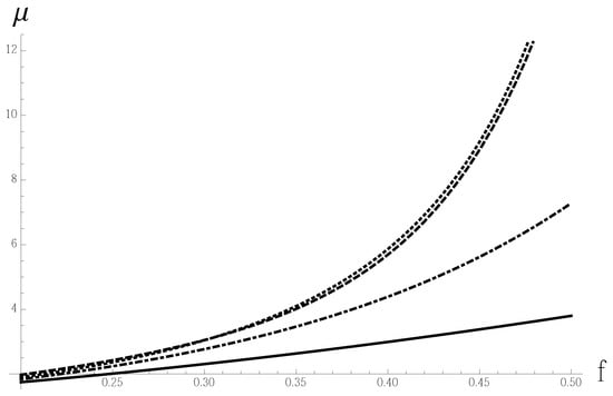
Figure 1.
Predictions for the effective viscosity (in the units of ) obtained with ARM after integration (12) applied to (55) (dotted) for passive suspensions. They are compared to the phenomenological Thomas formula (64) (dashed), an earlier RG-based result (70) (dot-dashed) and asymptotic expansion (44) (solid).
3. Effective Viscosity of Suspensions of Pullers
Pullers are an important biophysical system that exhibit a range of interesting macroscopic behaviors, while being in many ways simpler than pushers [21]. Their rheology could be similar to that of passive suspensions. It is believed that suspensions of puller-like microswimmers, such as Chlamydomonas algae cells, possess interesting rheological properties [41,42].
However, the pullers are difficult to investigate experimentally. At meaningful concentrations, the algae tend to form a kind of precipitate. Pullers typically propel themselves by executing a breaststroke-like motion with a pair of flagella attached at the front of the body (see, e.g., [43]). This should be contrasted to the propulsion of pushers, see Figure 2, which illustrates the two types of swimmers. The pushers, such as Escherichia Coli bacteria, use a rotating flagella bundle to push the fluid behind the bacterial body (see, e.g., [44]).
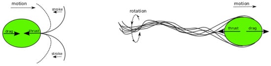
Figure 2.
Schematic depiction of swimmers. Left: a puller with two flagella executing a “breaststroke”. Right: a pusher swimming with a flagellar bundle acting as a “propeller”. Solid arrows show forces acting on the fluid.
The rheological behavior of pushers at present appears to be beyond the reach of analytical methods. Early experiments on pushers revealed a number of novel macroscopic properties of their suspensions. In particular, in [45,46], pushers were found to exhibit a super-diffusion for small times, with a crossover to classical diffusion on longer time intervals. This initial dramatic modification in diffusion was attributed to the advection generated by coherent bacterial motion. The second effect corresponds to the long-time diffusion enhancement compared to the passive case. The same effect was found for pullers, but in that case, it was shown to be much smaller [47,48].
The effect of different types of propulsion is even more pronounced in effective viscosity. For pushers, EV can decrease dramatically with the increasing particle concentrations but still remain in the dilute regime [12,49]. Even leading to a viscous-less, “super-fluid” regime with or even negative [49].
Experimental and theoretical models have been developed to examine fundamental aspects of a collective motion exhibited by various biological systems. Following the papers [12,50,51,52] and works cited therein, it was suggested that hydrodynamic interactions between the swimmers lead to the collective motion when every bacterium (pushers) interacts with others through the viscous environment. Implicit evidence of the collective motion can be found in a reduction in the effective viscosity [12]. The theoretical investigations of the collective motion were based on the framework of mechanical dynamical systems [53,54,55,56,57].
Experimental EV measurements for pullers are scarce, yet there are good reasons to expect [41] that pullers behave similarly to passive suspensions with a strongly enhanced effective viscosity [41,42]. In experiments on Chlamydomonas [41], this enhancement was found to be of a smaller magnitude than the corresponding EV decrease for pushers.
In a suspension of microscopic particles, both the strain-rate and the stress are modified by the disturbance flow around the particles, and the effective viscosity quantifies the relationship between these volume-averaged quantities. Operationally, we can define a scalar as relating fixed components of e and (e.g., the -components for particles suspended in a planar shearing flow) [44]. Given the low Reynolds numbers typical of suspensions, one has to solve the Stokes equation in the exterior of the microscopic particles. The solution amounts to balancing the forces and torques on the fluid. In the simplest case of dilute suspensions, the inclusions are statistically independent and do not interact. In this situation, the disturbance flow of a single typical particle is sufficient to determine the EV, and the normalized correction appears to be linear in the volume fraction of inclusions f.
The aspect ratio for prolate spheroids is quantified by the Bretherton constant , in terms of its minor and major semi-axes a and b. The dynamics of particle orientations in a linear ambient flow were elucidated by Jeffery (1922). When the particles are subject to the Brownian motion, a unique long-time distribution of orientations can be obtained, predicting only an increase in EV. For self-propelled particles modeled as prolate spheroids with a rigidly attached point force (see Figure 3), the situation is different. Elongated particles, according to Jeffery (1922), will spend more time aligned to the stable principal axis of the ambient planar shear flow.
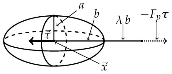
Figure 3.
A bacterium modeled as a prolate spheroid with semi-axes a and b, orientation and a point force “propeller” attached at distance behind the center of mass , pushing the fluid behind the bacterium.
Having established the ARM for passive suspensions, we would like to apply the same technique to suspensions of swimming cells. Specifically, it is important to suggest the concentration dependence of EV for suspensions of a puller cell organism. The interesting characteristic of pullers is that their presence tends to monotonically increase the effective viscosity of the suspension. The latter property is in contrast with pushers. The effective viscosity of pushers may depend on concentration non-monotonically and even exhibit a significant lowering of the effective viscosity for low to moderate concentrations.
However, one would expect all swimming cells or bacteria to affect the effective viscosity of the suspension similarly. All swimmers inject energy into the fluid, thus decreasing the effective rate of viscous dissipation and leading to an effective decrease in viscosity. The usual qualitative explanation of the different behavior of pullers is as follows. In an imposed shear flow, passive elongated particles approximated by infinitesimal rods—force dipoles—tend to align with the extensional axis of the flow, and the effective viscosity is increased. When a puller, approximated by a contractile dipole, is aligned with the extensional axis, the rate of strain is decreased. Since the viscosity is inversely proportional to the rate of strain, one can think that under a constant external force, the effective viscosity should increase.
Let us keep in mind that reconstruction of EV for pullers should be accomplished only on the basis of the (effective) intrinsic viscosity,
Even then, the problem is far more complicated than for passive systems since: (1) For comparison with experiments, has to be calculated first as a function of the puller’s internal parameters and of the flow. Second, (2) it should be supplemented with the information or insight on critical behavior at the dense packing limit, which we argue to be similar to that of passive suspensions.
Only then, would we be in a position to apply the techniques developed for passive suspensions and justify all the extensive groundwork on passive systems with only available from the “microscopic” approach of Stokes equations. To reconstruct the dependence of the intrinsic viscosity on the parameters of the background flow and the shape of the swimmers, we are going to rely on the results of [44]. In the paper [44], it was shown how the case of pullers can be obtained from the same formulae as for pushers just by changing the rigidly attached propulsion force . The analytical expressions for the intrinsic viscosity as a function of the arbitrary strain rate of the background flow, as well as the Bretherton constant, were obtained in [44], in the form of another two asymptotic pieces.
For the small parameter , applicable when the background flow is much smaller than the rotational diffusion of pullers (weak flow regime), the following asymptotic is valid,
with
Here, is a tumbling constant specifying the strength of rotational diffusion.
For the large , the background flow dominates the rotational diffusion (strong flow regime), and a different asymptotic is valid,
Coefficients , S and N are the shape factors, dependent only on the geometry of the puller [44]. In the aligned limit of a strong flow, the particles tend to align along the extensional axis of the flow.
It just so happens that the experimental data from [41] are outside the asymptotic regimes of (73) and (75). The only way to obtain estimates for the viscosity at real parameters is to find a good or just reasonable interpolation formula between these asymptotic regimes by means of yet another interpolation step with respect to the parameter . It seems convenient to separate the passive and active contributions to the effective intrinsic viscosity.
Therefore, we start with the construction of the suitable interpolation in the form
which is the simplest two-point Padé approximant (see, e.g., book [3]). The second approximant
is the simplest exponential interpolation.
We next form a mixture of the two approximants using the method of weighted averaging, according to the (56),
using the remaining condition—matching —to determine p:
where and are second-order terms in the expansion of and in the parameter , respectively.
A curve drawn for pullers with positive (see Figure 4) [21] demonstrates that the effective intrinsic viscosity always remains positive for pullers. It approaches the aligned limit from above and another limit of small from below.
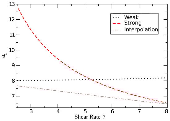
Figure 4.
The intrinsic viscosity of pullers as a function of strain rate magnitude : asymptotic results (weak, strong) and the weighted approximant (78) (interpolation).
The asymptotic expressions in [44] were derived in the absence of interactions between particles and yield only the intrinsic viscosity . Instead, just as is the case of passive suspensions, we apply the ARM to the first-order expansion in concentration with .
To complete the application of the ARM, the information on critical point behavior is required. Intuitively, the densely packed regime with power-law divergence can be invoked here. Indeed, for large concentrations, the algae cells become immobilized and nearly spherical [41], apparently falling dormant in the untenable conditions of very high concentrations. Thus we can apply the techniques developed for passive spherical particles, such as factor approximant from (58) using the intrinsic as the first-order coefficient.
The approximant is a function of both f and , describing the two crossovers, (1) with increasing , from zero to infinity, inside of the expression for the intrinsic viscosity, and (2) with increasing f from the active system at small f to the passive system at .
The first crossover was already formalized above by means of weighted averages of the two simple approximations. In the course of formalizing the second crossover, we have to rely on the approximants already tested above in the passive case.
For instance, the factor approximant provides a lower bound on our estimates of the EV of pullers. The very same expression as derived for the passive case is to be applied in the active case of pullers, but with replaced by for arbitrary . After the two crossovers are taken into account, the final expression should work, in principle, for arbitrary f and .
To assess the quality of the resulting prediction, we calculated the predicted enhancement in the effective viscosity relative to the passive spherical case. In practice, one can use the most transparent ARM approximant given by (46), with coefficients from (14). The only difference is that is replaced with from (78), so that it becomes . The enhancement ratio for this approximant becomes particularly transparent
To calculate the enhancement, we used the following parameters of the puller model (see Figure 3): the major semi-axis of the approximating spheroid , force location characterized by , bacteria’s swimming speed , rotational diffusion taken from [41,43]. Finally, the Stokes drag law holds, i.e., , where an expression for a factor N can be found in [44].
Let us finally make the desired estimates of the enhancement for the typical values of parameters of the problem, following [21]. For , and (motivated by an estimate of flagellar’ length, 10–12 , see [58]), the enhancement is around . The first-order renormalized coefficient is estimated as , and the second-order coefficient . Both numbers appeared as rather different from the corresponding numbers for passive systems.
When the enhancement ratio is averaged over various models, including the factor approximant, three ARM models and the KD model, it becomes larger and equals . The ratio also depends weakly on in agreement with the results on shear-thinning from [59]. Mind that all models involved in the averaging are based on the first-order expansion in concentration. Hence, the structure of the starting sections is dedicated in large part to such models.
It is interesting to realize, at least in principle, that an increase in the effective viscosity for pullers could have matched the corresponding decrease in the effective viscosity for pushers [44]. If is decreased to in accordance with [42], the average enhancement ratio increases to in good agreement with [41] and also could become considerably larger for smaller . For instance, for , we are able to estimate an increase of seven times the ratio, matching the corresponding decrease in the effective viscosity for pushers [21].
4. Critical Index for 3D Elasticity, or High-Frequency Viscosity
In the problem of finding the effective shear modulus of perfectly rigid spherical inclusions embedded at random into an incompressible matrix, we have two shear moduli, , G, for the particles and matrix, respectively, and the is going to be set to infinity. The jamming regime sets in when f tends to a random close packing fraction , and is very hard to simulate numerically. Therefore, the value of theoretical approaches to this limit is increasing.
The elasticity problem is treated by analogy to the problem of high-frequency effective viscosity of a suspension [60]. In the analogous case of suspension, consisting of hard spheres immersed in a Newtonian fluid of viscosity , only hydrodynamic interactions between pairs of suspended particles are considered.
For such suspension (or elastic composite), which is described by the ratio of the effective shear modulus to that of the matrix, and for small f, the second-order truncation is available [35],
The coefficient was also estimated earlier by Batchelor and Green, who gave [60]. In the vicinity of the 3D threshold, the effective modulus characteristically behaves as a power-law
where , [30,33]. Here stands for the critical index for 3D (super)elasticity, analogous to the critical index for the viscosity when only hydrodynamic interactions are considered.
The idea of application of optimal conditions in the space of approximations was put forward by V.I. Yukalov [61,62], and the minimal difference condition was formulated in [63]. The minimal derivative (sensitivity) condition was discussed in [64]. Kleinert also employed minimal derivative conditions in the course of his variational-perturbation method [65]. Technically, it is very difficult to extract expressions for the physical quantities in a closed form by Kleinert’s methods.
4.1. Original Suggestion
Let us recapitulate the original suggestion for the calculation of the critical index [66,67]. In the case of a critical quantity divergent at the critical point, one has to apply a resummation technique to the inverse series
where , . Here, we construct the simplest pair of approximations given below, with m being a control parameter,
The, we set to have the same behavior at infinity.
Let us have the two solutions (83) differ minimally in the vicinity of a critical point. The minimal difference condition between the two approximations is reduced to the condition on m,
where the threshold as a function of m,
was found from the first-order approximant. With the concrete parameters pertaining to the problem, we calculate . The corresponding critical index is found automatically.
4.2. Conditions on Thresholds
One can also select the iterated root as the second approximant, so that
where
The second-order approximant gives an explicit expression for the threshold,
The same threshold is expected for each approximation, i.e.
From (87), find the stabilizer m,
The critical index is determined by the control parameter, .
4.3. Conditions on the Critical Index
Let us consider the value of a threshold as a parameter . It could be introduced into consideration through the Euler transformation [4,68],
applied to the original truncation (81).
Let us begin by deriving the two low-order approximations,
After such a task is accomplished, it remains to minimize the difference
with respect to the control parameter where and are explicit formulas for the critical index obtained from the two approximations. Their difference can be minimized at a calculated value of threshold . The first-order approximant
gives the critical index .
4.4. Conditions on the Amplitude
Assume now that we know the correct value of threshold in advance, and try to use the knowledge in the course of estimating the index. Let us apply the Euler transformation (7), with known threshold . The original truncation is transformed to the following form,
The lower-order approximation can be written down as follows,
In order to construct a second approximation, we leave the constant outside of the renormalization procedure and obtain
Let us require that both approximations (90) and (91) have the same power-law behavior as so that
The parameter has to be deduced from the two approximants. Require now the fastest convergence of the two approximations, and impose the minimal difference condition on critical amplitudes. The solution to the minimization problem [4,68] is found so that . As usual, more details can be found in [4,68], where the case of elastic modulus is explained.
4.5. Minimal Derivative
We also may start with the iterated root employed for the second-order approximant,
where
The control parameter may be interpreted as the “critical” index in the vicinity of the (quasi)threshold . The second-order approximant (92) allows for an explicit expression for the quasi-threshold
Let us ask for an independence of the critical index at infinity on the position of a quasi-threshold. One can find the value of from the minimal derivative (sensitivity) condition imposed on the quasi-threshold,
and we found the critical index [4,68].
In summary, we found five fairly close estimates for the critical index . Their average equals , which is in fair agreement with the experiment [30]. Finer details and explanations can be found in [4,68].
4.6. Comment on the Method of Coherent-Anomaly
It is interesting to compare our results for the critical index with other approaches with similar objectives, such as the coherent-anomaly method (CAM) of Suzuki. CAM derives the critical index from a couple of systematically obtained approximations for the sought quantity, whose critical points converge to the known true value of . The physical idea behind initial CAM is to first take into account the diluted regime (long-range interactions) and to correct it by taking into account progressively larger clusters with shorter-range interactions. At each step, the problem becomes more difficult, but the result is still a mean-field approximation for the critical index with the expected critical index for any finite cluster.
Assume that the problem of finding the effective property is solved analytically for a number of finite clusters of varying size, including all the interactions between the growing number n of particles at each step. One can think about the regular or randomly generated clusters or about the snapshots of the real material. In application to elasticity, the problem would consist of the numerical extrapolation of the results for the effective moduli of such clusters to the infinite cluster as n tends to infinity.
Is it possible to move beyond the mean-field approximation within the framework of the cluster approach? The answer is “no” if only finite-size clusters are considered without additional efforts to make an inference on the case of infinite clusters. Suzuki suggested that additional information about the critical index is hidden in the parameters of two successive approximations [69]. In order to extract the information, one has to find the approximate thresholds and and the amplitudes and , i.e., the derivatives calculated in the vicinity of the approximate thresholds in each approximation. Then, the critical index value, different from the mean-field value, could be estimated. With increasing complexity of the approximation, the value of the threshold is supposed to approach the true threshold, and the value of the amplitude is supposed to increase, reflecting the so-called coherent anomaly.
The CAM is built in the same spirit as any renormalization group (RG), but the flow of the sought quantity is considered with respect to the approximation parameter, discrete or continuous. The critical amplitude of the mean-field approximation is considered the sought physical quantity. The value of amplitude should be known for at least two successive approximations. In addition, for the amplitude, it is most important that one should introduce a scaling hypothesis, which postulates that the amplitude diverges as a power-law with the index of in the vicinity of the fixed point with exact threshold . The divergence rate should give a non-mean-field contribution to the critical index on top of the mean-field value.
The scaling hypothesis, in turn, should be expressed in terms of the parameter characterizing proximity to the true critical point, or more generally, a fixed point of various RG transformations. To this end, one should know how such a parameter varies from approximation to approximation. It is enough to know the derivative of such transformation in the vicinity of the fixed point. When the ratio of amplitudes for two successive approximations is expressed in two different ways, one arrives at the formula for the critical index to be found as the solution of a simple equation. CAM recommends the simplest and most natural choice of the approximate threshold as the parameter characterizing the different approximations, and the derivative is simply expressed in finite differences between the two thresholds and the exact threshold. From the approximate thresholds and known amplitude ratios, one can express the critical index.
The final expression for the critical index becomes explicit and simple, as is expressed below
Here, the value of unity comes from the mean-field approximation and from the unaccounted interactions. This formula written in appropriate variables is standard for most RG calculations of the critical indices [70], except for the approaches of the type of [66], where the critical index is treated as a control parameter and found from some sort of additional condition of a non-perturbative nature.
We applied the two methods suggested by Suzuki to generate systematic mean-field approximations from the series. The first method of [71] is based on an analysis of the series and by studying the zeroes for the first two polynomials of the power-series of the inverse of the relevant physical quantity, giving and . Then, the mean-field amplitudes and can be found near each of the points.
Because we are working with inverse quantities, the value of amplitude decreases with an increasing number of terms. The critical exponent is estimated on the basis of the general CAM theory [69,72] and formula (94) with changed sign, with the result , for .
In the second method of [73], one should first construct the continued fractions, approximant asymptotically equivalent to the original series. Then, find the critical point from the position of the simple pole and determine the critical coefficient/amplitude as the corresponding residue so that
The information extracted from the two continued fractions is then combined with the CAM theory to estimate fractional critical exponents [69,72] from formula (94), with the result . The value of the critical coefficient now is increasing with an increasing number of terms, as is anticipated in the framework of CAM, and formula (94) is fully applicable.
The techniques of Padé approximants and their various modifications are rather popular, and their advantages and limitations are understood. Thus, first applying the diagonal Padé approximants or continued fractions as the zero approximation for the critical point should be quite natural. However, in an unexpected turn, the value of a critical index can also be found from such a pedestrian approach. However, it is given only implicitly, as it is hidden or scattered within the different Padé approximants.
The CAM estimates agree with other estimates from this section and are close to the upper bound. Such an estimated critical index could be employed as an initial guess/input for some other technique, which would operate with the critical index explicitly. Such a technique would calculate a correction to the CAM value and reconstruct corresponding improved approximants, giving the expression for the sought quantity for all concentrations.
5. Sedimenatation and Particle Mobility
The sedimentation problem is concerned with a suspension movement under gravity. The suspension is built of small rigid spheres with random positions, and they are falling through Newtonian fluid under gravity. A homogeneous mixture of solid particles and a fluid stands in a container. The rate of particles settling under gravity depends on their concentration, which is dependent on the hydrodynamic interaction between particles.
The quantity of interest is called sedimentation velocity U. It is nothing else but the averaged velocity of suspended particles. It is usually normalized with respect to the velocity of a single particle movement in the absence of any other particles. The ratio is also called the collective mobility or sedimentation coefficient. In sedimentation experiments, two different scenarios are played out. The first scenario corresponds to the phase transition [74], but different scenarios with metastable phase extension up to RCP [75] can be observed as well.
Below, we mainly follow the discussion presented in [4,68], present some empirical and semi-empirical observations, and develop formulas based on some low-order expansions for the sedimentation rate. We also provide some estimates for the critical properties of the sedimentation rate. Based on Stokes relation , where is an ambient fluid viscosity, one might expect the sedimentation rate to be inversely proportional to the effective viscosity of the suspension
One can think that the critical index value for the sedimentation rate is close to the critical index for effective viscosity. Various studies [76,77,78,79,80,81] suggest a critical behavior for the sedimentation rate in the form of formula (7),
with a positive critical index in the range from to . Various formulas for the sedimentation rate can be found in [4]. For small f, the following single-term expansion formula was found in [77]
The value of will be estimated below, following [4]. It turns out that the estimated value is in rather good agreement with some other microscopical, theoretical estimates.
We are interested in accurate expressions satisfying (97), with power-law behavior (96). Let us follow the method of derivation, which leads to formula (19). Let us find for the simplest approximant with fixed position of singularity and given the critical index [4],
From formula (98), one can find the approximate value of the second-order coefficient, i.e., . One can also estimate .
Another simple formula can be obtained similarly to the derivation of ([21], eq. 3.6),
and its expansion at small f gives a close value for . Both estimates for , especially the former, agree with the value of calculated in [82].
In reverse, accepting the theoretical estimate of , we can find
and estimate that . The latter value is exactly the result of the application of the diff-log Padé method from [4,68], after Euler transformation (7), from the finite interval to semi-infinity. After the transformation, one can simply apply the technique sketched in the end of Section 2.1. The new formula (98) agrees better in comparison with the simulation results of [80].
We conclude that the value of from the [82] is reasonable. We also employed it for more detailed estimates of the critical properties. Following minor modifications to the same approach of the five methods of application, as in Section 4, we found [68]. More details are presented below in Section 5.1. Keep in mind that in [33], we estimated the critical index
Practitioners also respect the formula suggested by Barnea–Mizrahi [83],
It works quite well in the region of high concentrations but gives different results as compared to the numerical data of [80].
5.1. Direct Estimates of the Critical Indices
In reverse, when the coefficient calculated in [82] is known in advance, so that for small f
one can estimate the value of a critical index at . Such an estimate is independent of any other experimental or theoretical considerations [68]. Let us again employ the special resummation techniques, just as in the previous section, for the shear modulus. In this case, for obtaining estimates of the critical index for the sedimentation rate, remember that the strategy consists of employing various conditions for the fixed point in order to compensate for a shortage of the coefficients. We present below only the main results obtained in [68].
The method of Section 4.1 gives the critical index .
The method of Section 4.2 produces an unreasonably large value and is discarded.
The method of Section 4.3 brings the critical index .
The minimal difference condition of Section 4.4 gives the index
The minimal derivative condition of Section 4.5 leads to the critical index .
The index can also be obtained with the diff-log Padé method of [4,68], with the result .
The average taken among all estimates gives the value of .
The formulas for the sedimentation rate U presented above are applicable up to before the freezing point for the hard-spheres suspension.
In the case of a metastable branch of the suspension, the following expression was derived in [4,68],
In the latter case, we looked for a formula to continue up to the jamming threshold of . The critical index was found for such a threshold in [4,68]. The latter value of appeared as close to the estimates for the critical index of the high-frequency effective viscosity due to hydrodynamic interactions, obtained in the preceding Section.
6. Non-Local Diffusion in Critical Liquids
The definition of a non-local diffusion coefficient in liquids and suspensions dwells on some other quantities, which are briefly discussed below. First, one has to introduce the space- and time-dependent local number density
where N stands for the number of particles.
Second, consider the intermediate scattering function, which is the auto-correlation function of the Fourier components [84],
where the averaging is performed over a statistical ensemble. depends on time t and on the wave-number q.
Even more convenient for experimental and theoretical purposes is the dynamic structure factor [85]. It is defined as the Fourier-transform of the in the temporal domain
The celebrated is directly measurable in light scattering experiments. The density fluctuations spectrum corresponds to the simple pole in , dependent on frequency and on the wave-number q. To obtain the non-local, q-dependent diffusion coefficient, one has to simply divide by [86].
Near the critical point, temperature is measured by the ratio . We are interested here only in long-time relaxation properties, dependent on the wave-number q. They are characterized by the characteristic relaxation time of the density fluctuations. Such fluctuations are the inverse of the .
The dynamic scaling hypothesis conjectures that the characteristic frequency can be expressed in the following form
Here, the dynamical critical index z is introduced, and stands for the inverse correlation length [38]. In fact, we are looking for an approximation for the function and would like to estimate the index z. The length scale is intermediate between the atomic and macroscopic scales.
The behavior of can be reconstructed approximately from some general asymptotic information [38] using the crossover approach of [24]. The scheme was extended and developed further in the book [4]. Crossovers are typical of the thermodynamics of a supercritical state [87].
In the hydrodynamic regime , for isotropic fluid, we have an expansion [38],
In the fluctuation regime , another expansion is considered,
The expansion is expounded in [38]. Here, is thermal diffusivity. The value of B is estimated as [38,88]. Assume also that the value of A is known.
The simple analytical expression for the characteristic frequency for arbitrary was suggested [24],
where C is constant, and
If we now substitute the dependencies of and into the expression for C, then the well-known relation
we simply recover the known relation between the dynamic critical index z and three other critical indices , and a. Formula (107) represents one of the central results of the dynamical scaling hypothesis [38]. Remember that stands for the critical index for heat capacity, while a stands for the critical index for thermal conductivity. Index is the correlation length critical index. The combination
stands for the critical index for thermal diffusivity.
From (106), it follows then that
in such a way that requirement =const is satisfied when the relation between indices (107) is valid.
The index is determined mainly by the concentration (long time) diffusion coefficient (see, e.g., [89]), which in turn, can be estimated from the analog of Stoke’s formula [4]. The value of is dominated by the correlation length index, provided the effective viscosity remains finite at the critical point as [4]. Therefore, .
Using the scaling relation (107), the dynamic critical index can be crudely estimated as . However, one can also take into account a correction to z, originating from weakly divergent viscosity. If such divergence is characterized by the index (measured in units of the critical index ), then
The latter formula means that it takes longer for short wavelength density fluctuations to relax if compared with a long wavelength regime. Different estimates for can be found in [90].
The unknown C can be estimated from the asymptotic equivalence with the expansion (103) in the hydrodynamic regime. For instance, , with typical B and z. To calculate the thermal diffusivity , one can simply use the diffusion coefficient approximated by the Stokes formula, as explained in [4,86,89].
The non-dimensional part of can be approximated already by a simple self-similar root approximant
where . Its asymptotic behavior as
respects the coefficient B, while as
Both expressions are in qualitative agreement with the expressions (103), (104). Expansions (109), (110) are designed to obey the dynamic scaling in all orders.
The non-dimensional part of
was derived by Kawasaki [88]. Its asymptotic behavior as
is qualitatively correct in all orders. It is in agreement with the dynamic scaling in the hydrodynamic limit (103).
While as
However, the second expansion (113) agrees only with the leading term in (104). This means that it violates the dynamic scaling by means of the term in (113). The term is altogether absent. We conclude that the Kawasaki approximation [88] is correct only as far as the leading term is considered in the limit-case of .
In the book [4], we attempted to find some form of approximant extending (108) based asymptotically on a few terms from the correct Kawasaki limit and the leading term as . Such approximants should be free from the terms violating dynamic scaling. In other words, we thrive on restoring dynamic scaling in all orders. To this end, we have to come up with some additional considerations.
Already, the simplest factor approximants give a reasonable approximation to the Kawasaki function while restoring the dynamic scaling in all orders [4]. Based on this observation, one can suggest a simple factor approximant to the non-dimensional part of , generalizing the simplest forms presented above to an arbitrary z (). In other words, the second-order factor approximant satisfies just one non-trivial coefficient from (112) and is designed to give the correct critical index,
The higher-order approximant asymptotically obeys the three non-trivial coefficients from (112) and also gives the correct critical index z. It also has a closed form but with expressions for the parameters given explicitly in [4],
Approximants (114) and (115) respect the dynamic scaling by design. Of course, they can also be used with a non-zero . In such cases, the Kawasaki function is not rigorously applicable. Remember that in developing the factor approximations, we rely on the fact that the Kawasaki approximation works well at small x, at least in leading orders [38]. However, the Kawasaki function is often used as a part of the formulas that account for the correct value of the critical index z. For instance, the following approximation was developed in [91],
Another formula was explored in [86,92,93],
In Figure 5, factor approximants (114) and (115) are compared with the two non-monotonous approximations based on the Kawasaki function and with reference to the monotonous Kawasaki function itself. They deviate from the Kawasaki (111) in less than two other semi-empirical formulas. Such a difference is potentially above the typical experimental error of [89].
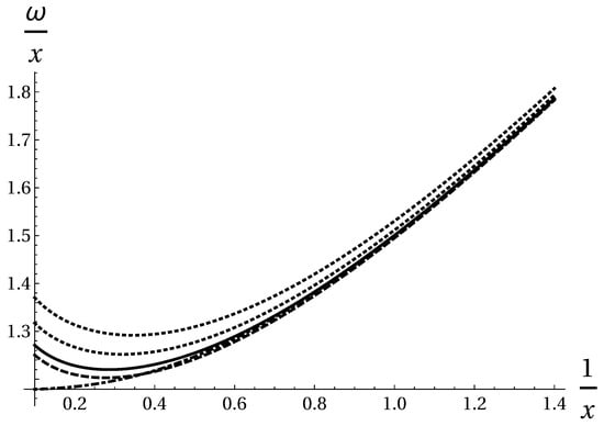
Figure 5.
The non-dimensional ratio is shown along the y-axis, dependent on the parameter . The lower-order factor approximant (114) divided by x is shown with a dashed line (). The higher-order factor approximant (115) divided by x is shown with a solid line, with the same . The expression (117) (dotted) corresponds to the lower curve. Formula (116) is also shown with a dotted line but correspondes to the upper curve. The Kawasaki formula (111) is also brought up and is shown with a dot-dashed line.
7. Effective Conductivity of a Classical Analog of Graphene
For the subsequent study, it is important to remember that graphene consists of atoms tightly packed into a 2D honeycomb lattice. Graphene has very good electric conductivity, at par with silver and copper. On the other hand, silver (or copper) inclusions, embedded into a very weakly conducting matrix (vacuum, air, water, polyfoam), can be considered perfect conductors [94].
Consider a continuum analog of graphene [68,94]. To this end, one can introduce and study a regular honeycomb array of perfectly conducting (superconducting) disks. The disks are embedded into a matrix with a conductivity normalized to unity. With respect to the matrix conductivity, one can set the inclusions conductivity to infinity. The relevance for establishing the analogy case corresponds to the volume fraction . In such a limit-case, one can expect that the effective conductivity of the array goes to infinity.
If some vacancies are introduced at random within the continuum model, the threshold , or maximal possible volume fraction of disks in a regular case, will be lowered to the value of , where the parameter p is the number of vacancies per cell and . The effective conductivity is expected to diverge with some critical index . For the sake of analogy, with graphene, it only makes sense to consider the limit [68,94].
The expansion for small f is possible to obtain by means of the Monte Carlo simulations combined with analytical results from the method of basic structural sums, as described in [94], leading to the polynomials representing effective conductivity at small and moderate f. The details of the methodology of deriving the effective conductivity of finite samples for various p can be found in [68,94]. A complete set of polynomials for can be found in [68].
For instance, in some particular cases, the following truncations were computed,
Smoothing of the polynomials was performed following the methodology explained in [94] in great detail. Concrete sets of polynomials for smaller samples can be found in [94]. Polynomials (118) can be seen as evolving smoothly from the expression (121) for the regular case with increasing p.
The critical index will be found by extrapolation from the small-f polynomials to . The threshold is conveniently given by formula (120). In the vicinity of the threshold, the following family of power-laws is considered
Here, the superconductivity critical index depends on p. We also expect that as , the index should be equal to .
The threshold also depends on p. It is given by the compact formula
where is the maximum volume fraction attainable for the honeycomb lattice, and the maximal value of p is denoted as . In simulations of [68], . When the threshold is known, we would first apply the following Euler transformation (7),
to the original series. The transformation maps the segment to a half-line.
It is instructive to first study the regular case with no defects. The small-f polynomial corresponding to the case of has the following form,
calculated exactly from the formulas of [3], applied to the case of a honeycomb array of disks. Let us calculate the critical index applying the technique suggested in Section 2.1.1. After the diff-log transformation, taking an inverse and Borel summation of Section 2.1.1, we arrive at the following sequence of approximations dependent on the number of terms k involved in the construction of the iterated roots,
The latter sequence can be continued beyond the fifth order if we also keep taking the inverse of the sixth order term, i.e., . The results agree rather well with the expected value of . The latter estimate seems better than the result of [68], which was obtained by the technique of the paper [33], as already employed in Section 2.1.2. Note that the method of [31], based on the Borel summation and factor approximants [31], failed to produce a convergent sequence.
Similarly, for the case of , we obtain the following sequence
The latter estimate agrees with the result of [68] for the same disordered case.
Again, similarly for the case of , we obtain the following sequence
The latter estimate agrees with the result of [68] for the same disordered case. The dependence of on the degree of disorder measured in steps p of randomization achieved through random placement of vacancies on a honeycomb lattice is displayed in Figure 6. The results given by the Borel summation method in the sixth order, as explained in the examples above, are shown with squares. The results found by applying the fifth-order Borel summation method are shown with disks.
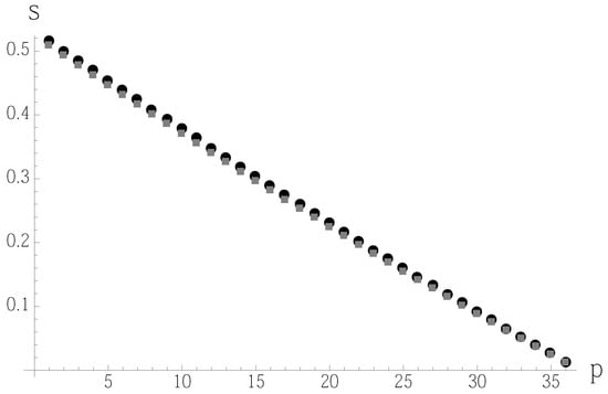
Figure 6.
The dependence of on the degree of disorder measured in steps p of randomization attained through random placement of vacancies on a honeycomb lattice is displayed. The results given by the approximants of the sixth-order procedure are shown with squares. The results found by applying the fifth-order approximation method are shown with disks.
We see that both approximations give rather close results for the index for all p.
One can also plot curves for the (inverse) effective conductivity [68,94] for varying p. The dependence is characterized by the steepening of the curves with an increasing fraction of vacancies [68,94], while the threshold simultaneously shifts to smaller values. The index is non-universal, smaller than , and decreases with increasing concentration of vacancies. Remarkably, the honeycomb array of highly conducting disks has the ability to adapt to randomly placed vacancies by adjusting (lowering) the threshold and critical index, effectively retaining its quasi-regularity. One can think that analogous graphene can also withstand the infusion of vacancies while remaining a good conductor.
The dependence of the critical index on the degree of disorder defies the universality hypothesis [95]. Similarly, the critical index in the so-called eight-vertex model and equivalent Ising model with four-spin interaction [95] depends on temperature [96].
It would also be very interesting to understand if there is a way to find a continuous analog of the order to disorder abrupt transition in quasi-periodic twisted bilayer graphene composites [97]. The interesting effect of order emerging from disorder was discovered in [98]. In both situations, it could be interesting to access the change in critical properties in the course of transitions.
8. Superconductivity Critical Index of Random 3D Composite
It was argued in [4] that in the limit-case of a random array of perfectly conducting spherical inclusions embedded into a matrix with a conductivity normalized to unity, the expression for effective conductivity , given by the classical Jeffrey formula [99], could possibly contain the wrong quadratic term in the volume fraction f.
Interesting and challenging analyses of various formulas in the theory of composites can be found in [100,101]. However, the effective medium-type approaches can be useful if applied properly for the qualitative analysis of the complex composite systems [102,103], when modeling is not feasible, when the system is designed particularly to satisfy the certain, generalized Hashin–Shtrikman bounds [104], or when the expansions are converging fast [105]. The method of basic structural sums developed by Mityushev et al. [3,4], serves as the firm foundation for obtaining polynomial truncations of the effective properties, as well as for the direct analysis of a micro-structure of nanocomposites [106].
For macroscopically isotropic composites, the following truncated expansion for effective scalar conductivity was found
Jeffrey [99], in this case gives, only a quadratic term, . Mityshev et al. concluded in [4] that such a disparity is caused by a methodological error, “related to an intuitive physical treatment of the conditionally convergent integral discussed in [99]”.
With a known threshold corresponding to the random close packing (RCP), , the conductivity is given by the power-law of the type (7),
From simulations, the superconductivity critical index is expected to have the value of [107]. Let us estimate the value of based on asymptotic information contained in (122). Let us use the same method for calculating the critical indices as in Section 2.1.2. To this end, compose the sequences , with . From the series (122), one can find only three independent estimates for the critical index , see Table 2. One can see that all three are close to and to the expected value of . More details can be found in the book [4].
Table 2.
Critical indices for the superconductivity obtained from the optimization conditions .
To obtain a final formula, one can simply fix the value of and find the following approximant for the effective conductivity:
From the approximant, we obtain . Furthermore, the fourth-order coefficient, , could be found from .
Let us calculate the critical index , applying the technique suggested in Section 2.1.1. After the diff-log transformation, inversion and Borel summation, we arrive at the following sequence of approximations dependent on the number of terms k involved in the construction of the iterated roots,
With the index fixed to the value of and applying the technique of [32] directly to the truncation (122), we obtain the following sequence of amplitudes
The latter sequence was continued beyond the third order since we kept going after the Euler variable transformation (7) to the fourth-order term.
The method of self-similar Borel summation [31] based on Borel transformation and factor approximants, and described in more detail in Section 2.1.1, produces reasonable values
for the index, and in the third order gives . Various techniques bring very close results for the critical index and amplitude.
9. Concluding Remarks
The conclusion of the paper is straightforward. Even short polynomial expressions derived by the great scientists for the effective properties at small values of relevant parameters are rather informative, as long as their treatment is complemented with the consideration of critical properties for a non-universal critical phenomenon. Such a particular realization of the L. I. Manevitch asymptotic complementarity principle (from the 1960s) [108] is our contribution to the “Big Picture”. Moreover, the two limit-cases are so thoroughly intertwined or entangled in the course of obtaining an approximate solution, that each of them retains hidden information about the other even when they are considered separate or disentangled. Uncovering such information turns out to be possible by means of mostly analytical tools. Thus, an analytical approach to perturbative problems advocated by Feynman and developed by Bogolyubov in the refined form of an RG turns out to be fruitful in application to the effective properties.
One can think about the methodological universality in place of the physical universality of critical phenomena elaborated on by Wilson and Kadanoff [6,70].
In Section 2, we applied the methods of estimation of the coefficients in the truncated expansions based on the first-order and second-order coefficients, supplemented by the information on the maximum volume fraction and critical indices for the effective viscosity. In the three-dimensional case, the critical index is even calculated based on the two non-trivial coefficients and threshold by applying the factor approximants. The results for the index are found to be in good agreement with Brady predictions. In the three-dimensional case, an accurate crossover formula for the conductivity is brought up. They are compared with others and are in good agreement with the reference formula.
In Section 3, the formulas developed in Section 2 for passive suspensions are applied to the active suspensions of puller micro-organisms. The two crossover problems for the intrinsic viscosity dependent on activity, and the effective viscosity dependent on volume fractions are solved approximately. The quality of approximations could be evaluated by estimating the enhancement in the effective viscosity, which turned out correct by an order of magnitude for pullers.
In Section 4, we discussed the main five methods for the problem of the calculation of the critical indices and amplitudes from extremely short truncated series. The critical index for the shear modulus of random elastic composites is calculated by all five methods, and the average (and variance) is found in agreement with expectations from the experiments.
In Section 5, the critical indices for sedimentation are calculated from the short truncation by means of minimal difference and minimal derivative conditions imposed directly on the critical properties. The estimates at various thresholds agree with other theoretical estimates and real experimental results.
In Section 6, we found the crossover expressions for the non-local diffusion coefficient of a simple liquid in the vicinity of a critical point, dependent on the wave-number of density fluctuations in the liquids. The extensions and corrections to the celebrated Kawasaki formula are designed in such a way that the dynamic scaling hypothesis is satisfied in all orders.
In Section 7, we calculated the effective critical index for superconductivity dependent on the concentration of vacancies. The index is predicted to be smaller than the value of for the two-dimensional regular composites.
In Section 8, we calculated the superconductivity critical index of the random three-dimensional composite in good agreement with results from simulations on lattice models.
The problems to be solved are technical but difficult, consisting of improvements of the quality of expansions using some smoothing procedures, such as those applied in the derivation of the expansions in [94]. Hopefully, a more accurate truncated expansion could be obtained for the problems of finding critical indices t for conductivity in 3D and elasticity in 2D and 3D cases [1,4].
The method of self-similar Borel summation could be improved further by applying it iteratively, with the number of iterations playing the role of a control. Generally speaking, the quality of Borel summation could be improved through various generalizations, and finding the most effective optimization technique, in addition to those already available [32], would help to improve the accuracy of summations in various problems of physics and applied mathematics.
Another challenge to be solved is envisaging a 2D system with a critical index for superconductivity larger than , as our work already covered the physics behind the region of [3,68,94].
Funding
This research received no external funding.
Institutional Review Board Statement
Not applicable.
Informed Consent Statement
Not applicable.
Data Availability Statement
Not applicable.
Acknowledgments
I am indebted to my Colleagues, P. Drygaś, D, Karpeev, P. Kyrtuka, V. Mityushev, W. Nawalaniec, N. Rylko, V. Yukalov whose contributions at different times made this review possible.
Conflicts of Interest
The author declare no conflict of interest.
Nomenclature
| f | stands for volume fraction (concentration) of the inclusions |
| stands for the critical index for superconductivity | |
| stands for frequency | |
| stand for the wave vector and wave number | |
| stands for the effective conductivity | |
| stands for the effective shear modulus | |
| is the critical index for super-elasticity and viscosity | |
| stand for the components of the strain tensor | |
| both stand for the effective viscosity | |
| stand for the components of the stress tensor | |
| 2D, and 3D | mean two-, and three- dimensional |
| A, B and C | stand for the critical amplitudes |
| stands for the factor approximants | |
| stands for the Padé -approximant | |
| stands for the root approximants | |
| KD | means Krieger–Dougherty equation |
| ARM | means algebraic renormalization method |
| CAM | means coherent-anomaly method |
| RG | means renormalization group |
| RCP | means random close packing |
| T | stands for temperature |
| generally stands for the critical index in application to an arbitrary case | |
| stands for the function | |
| stands for the exponential integral | |
| ∼ | indicates asymptotic equivalence between functions, i.e., indicates that functions are similar, of the same order |
| ≃ | indicates that the two functions are similar or equal asymptotically |
| ≈ | is used as “approximately equal to”, indicating that the number is acceptably close to an exact value |
| marks self-similar approximants |
References
- Torquato, S. Random Heterogeneous Materials: Microstructure and Macroscopic Properties; Springer: New York, NY, USA, 2002. [Google Scholar]
- Andrianov, I.V.; Awrejcewicz, J.; Danishevskyy, V.V. Asymptotical Mechanics of Composites. Modelling Composites without FEM; Springer Nature: Cham, Switzerland, 2018. [Google Scholar]
- Gluzman, S.; Mityushev, V.; Nawalaniec, W. Computational Analysis of Structured Media; Academic Press (Elsevier): Amsterdam, The Netherlands, 2017. [Google Scholar]
- Drygaś, P.; Gluzman, S.; Mityushev, V.; Nawalaniec, W. Applied Analysis of Composite Media; Woodhead Publishing (Elsevier): Sawston, UK, 2020. [Google Scholar]
- Torquato, S. Extraordinary disordered hyperuniform multifunctional composites. J. Compos. Mater. 2022, 56, 3635–3649. [Google Scholar] [CrossRef]
- Ma, S. Theory of Critical Phenomena; Benjamin: London, UK, 1976. [Google Scholar]
- Gluzman, S. Nonlinear Approximations to Critical and Relaxation Processes. Axioms 2020, 9, 126. [Google Scholar] [CrossRef]
- Klatt, M.A.; Steinhardt, P.J.; Torquato, S. Gap Sensitivity Reveals Universal Behaviors in Optimized Photonic Crystal and Disordered Networks. Phys. Rev. Lett. 2021, 127, 037401. [Google Scholar] [CrossRef] [PubMed]
- Torquato, S. Diffusion spreadability as a probe of the microstructure of complex media across length scales. Phys. Rev. E 2021, 104, 054102. [Google Scholar] [CrossRef]
- Torquato, S. Perspective: Basic understanding of condensed phases of matter via packing models. J. Chem. Phys. 2018, 149, 020901. [Google Scholar] [CrossRef] [PubMed]
- Martys, N.S. Study of a dissipative particle dynamics based approach for modeling suspensions. J. Rheol. 2005, 49, 401–424. [Google Scholar] [CrossRef]
- Sokolov, A.; Aranson, I. Reduction of effective viscosity in suspension of swimming bacteria. Phys. Rev. Lett. 2009, 103, 148101. [Google Scholar] [CrossRef]
- Ding, J.; Warriner, H.E.; Zasadzinski, J.A. Viscosity of two-dimensional suspensions. Phys. Rev. Lett. 2002, 88, 168102. [Google Scholar] [CrossRef]
- Alonso, C.; Waring, A.; Zasadzinski, J.A. Keeping lung surfactant where it belongs: Protein regulation of two-dimensional viscosity. Biophys. J. 2005, 89, 266–273. [Google Scholar] [CrossRef]
- Prasad, V.; Weeks, E.R. Two-dimensional to three-dimensional transition in soap films demonstrated by microrheology. Phys. Rev. Lett. 2009, 102, 178302. [Google Scholar] [CrossRef]
- Brady, J.F. The Einstein viscosity correction in n dimensions. Int. J. Multiph. Flow 1984, 10, 113–114. [Google Scholar] [CrossRef]
- Belzons, M.; Blanc, R.; Boumlot, J.L.; Camoin, C. Viscosite d’une suspension diluee et bidimensionnelle de spheres. C. R. Acad. Sci. Paris 1981, 292, 939–944. [Google Scholar]
- Bouillot, J.L.; Camoin, C.; Belzon, M.; Blanc, R.; Guyon, E. Experiments on 2-D suspensions. Adv. Colloid Interface Sci. 1982, 17, 299–305. [Google Scholar] [CrossRef]
- Bicerano, J.; Douglas, J.F.; Brune, D.A. Model for the viscosity of particle dispersions. Polym. Rev. 1999, 39, 561–642. [Google Scholar] [CrossRef]
- Olsson, P.; Teitel, S. Critical Scaling of Shear Viscosity at the Jamming Transition. Phys. Rev. Lett. 2007, 99, 178001. [Google Scholar] [CrossRef]
- Gluzman, S.; Karpeev, D.A.; Berlyand, L.V. Effective viscosity of puller-like microswimmers: A renormalization approach. J. R. Soc. Interface 2013, 10, 20130720. [Google Scholar] [CrossRef]
- Altenberger, A.R.; Dahler, J.S. A renormalization group calculation of the viscosity of a hard-sphere suspension. J. Colloid Interface Sci. 1997, 189, 379–381. [Google Scholar] [CrossRef]
- Gluzman, S.; Yukalov, V.I. Algebraic self-similar renormalization in theory of critical phenomena. Phys. Rev. E 1997, 55, 3983–3999. [Google Scholar] [CrossRef]
- Gluzman, S.; Yukalov, V.I. Unified approach to crossover phenomena. Phys. Rev. E 1998, 58, 4197–4209. [Google Scholar] [CrossRef]
- Gluzman, S.; Yukalov, V.I. Self-similar extrapolation from weak to strong coupling. J. Math. Chem. 2010, 48, 883–913. [Google Scholar] [CrossRef]
- Yukalov, V.I.; Gluzman, S. Self-similar bootstrap of divergent series. Phys. Rev. E 1997, 55, 6552–6570. [Google Scholar] [CrossRef]
- Hwang, W.; Hulse, M. Direct numerical simulations of hard particle suspensions in planar elongnational flow. J. Non-Newton. Fluid Mech. 2006, 136, 167–178. [Google Scholar] [CrossRef]
- Doyeux, V.; Priem, S.; Jibuti, L.; Farutin, A.; Ismail, M.; Peyla, P. Effective viscosity of two-dimensional suspensions: Confinement effects. Phys. Rev. Fluids 2016, 1, 043301. [Google Scholar] [CrossRef]
- Brady, J.F. The rheological behavior of concentrated colloidal dispersions. J. Chem. Phys. 1993, 99, 567–581. [Google Scholar] [CrossRef]
- Losert, W.; Bocquet, L.; Lubensky, T.C.; Gollub, J.P. Particle dynamics in sheared granular matter. Phys. Rev. Lett. 2000, 85, 1428–1431. [Google Scholar] [CrossRef] [PubMed]
- Yukalov, V.I.; Gluzman, S. Methods of Retrieving Large-Variable Exponents. Symmetry 2022, 14, 332. [Google Scholar] [CrossRef]
- Gluzman, S. Optimal Mittag-Leffler Summation. Axioms 2022, 11, 202. [Google Scholar] [CrossRef]
- Gluzman, S.; Yukalov, V.I. Critical indices from self-similar root approximants. Eur. Phys. J. Plus 2017, 132, 535. [Google Scholar] [CrossRef]
- Batchelor, G.K. The effect of Brownian motion on the bulk stress in a suspension of spherical particles. J. Fluid Mech. 1977, 83, 97–117. [Google Scholar] [CrossRef]
- Wajnryb, E.; Dahler, J.S. The Newtonian viscosity of a moderately dense suspensions. In Advances in Chemical Physics; Prigogine, I., Rice, S.A., Eds.; Wiley: New York, NY, USA, 1997; Volume 102, pp. 193–313. [Google Scholar]
- Wang, M.; Brady, J.F. Constant stress and pressure rheology of colloidal suspensions. Phys. Rev. Lett. 2015, 115, 158301. [Google Scholar] [CrossRef]
- Haines, B.M.; Mazzucato, A.L. A proof of Einstein’s effective viscosity for a dilute suspension of spheres. SIAM J. Math. Anal. 2012, 44, 2120–2145. [Google Scholar] [CrossRef]
- Stanley, H.E. Introduction to Phase Transitions and Critical Phenomena; Oxford University Press: Oxford, UK, 1971. [Google Scholar]
- Thomas, D.G. Transport characteristics of suspension:VIII. A note on the viscosity of newtonian suspensions of uniform Spherical Particles. J. Colloid Sci. 1965, 20, 267–277. [Google Scholar] [CrossRef]
- Song, Y.; Zheng, Q. A Guide for Hydrodynamic Reinforcement Effect in Nanoparticle-filled Polymers. Crit. Rev. Solid State Mater. Sci. 2016, 41, 318–346. [Google Scholar] [CrossRef]
- Rafai, S.; Jibuti, L.; Peyla, P. Effective viscosity of microswimmers suspensions. Phys. Rev. Lett. 2010, 104, 098102. [Google Scholar] [CrossRef]
- Mussler, M.; Rafai, S.; Peyla, P.; Wagner, C. Effective viscosity of non-gravitactic Chlamydomonas Reinhardtii microswimmer suspensions. Europhys. Lett. 2013, 101, 54004. [Google Scholar] [CrossRef]
- Drescher, K.; Dunkel, J.; Cisneros, L.; Ganguly, S.; Goldstein, R. Fluid dynamics and noise in bacterial cell-cell and cell-surface scattering. Proc. Natl. Acad. Sci. USA 2011, 108, 10940. [Google Scholar] [CrossRef]
- Haines, B.M.; Aranson, I.; Berlyand, L.; Karpeev, D. Effective viscosity of bacterial suspensions: A three-dimensional PDE model with stochastic torque. Comm. Pure Appl. Anal. 2012, 11, 19. [Google Scholar] [CrossRef]
- Wu, X.L.; Libchaber, A. Particle diffusion in a quasi-two-dimensional bacterial bath. Phys. Rev. Lett. 2000, 84, 3017–3020. [Google Scholar] [CrossRef]
- Hernandez-Ortiz, J.; Stoltz, C.; Graham, M. Transport and collective dynamics in suspensions of confined swimming particles. Phys. Rev. Lett. 2005, 95, 204501. [Google Scholar] [CrossRef]
- Underhiil, P.; Hernandez-Ortiz, J.; Graham, M. Diffusion and spatial correlations in suspensions of swimming particles. Phys. Rev. Lett. 2008, 100, 248101. [Google Scholar] [CrossRef]
- Leptos, K.; Guasto, J.; Gollub, J.; Pesci, A.; Goldstein, R. Dynamics of enhanced tracer diffusion in suspensions of swimming eukaryotic microorganisms. Phys. Rev. Lett. 2009, 103, 198103. [Google Scholar] [CrossRef] [PubMed]
- Lopez, H.M.; Gachelin, J.; Douarche, C.; Auradou, H.; Clement, E. Turning bacteria suspensions into a “superfluid”. Phys. Rev. Lett. 2015, 115, 028301. [Google Scholar] [CrossRef]
- Sokolov, A.; Aranson, I.S.; Kessler, J.; Goldstein, R. Concentration dependence of the collective dynamics of swimming bacteria. Phys. Rev. Lett. 2007, 98, 158102. [Google Scholar] [CrossRef] [PubMed]
- Sokolov, A.; Goldstein, R.E.; Feldstein, F.I.; Aranson, I.S. Enhanced mixing and spatial instability in concentrated bacteria suspensions. Phys. Rev. E 2009, 80, 031903. [Google Scholar] [CrossRef] [PubMed]
- Sokolov, A.; Aranson, I.S. Physical properties of collective motion in suspensions of bacteria. Phys. Rev. Lett. 2012, 109, 248109. [Google Scholar] [CrossRef] [PubMed]
- Ryan, S.D.; Haines, B.M.; Berlyand, L.; Ziebert, F.; Aranson, I.S. Viscosity of bacterial suspensions: Hydrodynamic interactions and self-induced noise. Phys. Rev. E 2011, 83, 050904(R). [Google Scholar] [CrossRef] [PubMed]
- Ryan, S.D.; Sokolov, A.; Berlyand, L.; Aranson, I.S. Correlation properties of collective motion in bacterial suspensions. New J. Phys. 2013, 15, 105021. [Google Scholar] [CrossRef]
- Ryan, S.D.; Berlyand, L.; Haines, B.M.; Karpeev, D.A. A kinetic model for semi-dilute bacterial suspensions. Multiscale Model. Simul. 2013, 11, 1176–1196. [Google Scholar] [CrossRef]
- Potomkin, M.; Gyrya, V.; Aranson, I.; Berlyand, L. Collision of microswimmers in viscous fluid. Phys. Rev. E 2013, 87, 053005. [Google Scholar] [CrossRef]
- Tournus, M.; Berlyand, L.V.; Kirshtein, A.; Aranson, I. Flexibility of bacterial flagella in external shear results in complex swimming trajectories. J. R. Soc. Interface 2014, 12, 102. [Google Scholar]
- Goldstein, R.E.; Polin, M.; Tuval, I. Noise and synchronization in pairs of beating eukaryotic flagella. Phys. Rev. Lett. 2009, 103, 168103. [Google Scholar] [CrossRef] [PubMed]
- Jibuti, L. Locomotion and Flow in Complex and Confined Fluids. Ph.D. Thesis, Université de Grenoble I, Grenoble, France, 2011. [Google Scholar]
- Batchelor, G.K.; Green, J.T. The determination of the bulk stress in a suspension of spherical to order c2. J. Fluid Mech. 1972, 56, 401–427. [Google Scholar] [CrossRef]
- Yukalov, V.I. Theory of perturbations with a strong interaction. Mosc. Univ. Phys. Bull. 1976, 51, 10–15. [Google Scholar]
- Yukalov, V.I. Model of a hybrid crystal. Theor. Math. Phys. 1976, 28, 652–660. [Google Scholar] [CrossRef]
- Kadanoff, L.P.; Houghton, A. Numerical evaluations of the critical properties of the two-dimensional Ising model. Phys. Rev. B 1975, 11, 377–386. [Google Scholar] [CrossRef]
- Stevenson, P.M. The effective exponent γ(Q) and the slope of the β-function. Phys. Lett. B 2016, 761, 428–430. [Google Scholar] [CrossRef][Green Version]
- Kleinert, H. Path Integrals in Quantum Mechanics, Statistics, Polymer Physics and Financial Markets; World Scientific: Singapore, 2006. [Google Scholar]
- Yukalov, V.I.; Gluzman, S. Critical indices as limits of control functions. Phys. Rev. Lett. 1997, 79, 333–336. [Google Scholar] [CrossRef]
- Gluzman, S.; Karpeev, D.A. Perturbative expansions and critical phenomena in random structured media. In Modern Problems in Applied Analysis; Drygas, P., Rogosin, S., Eds.; Birkhäuser: Basel, Switzerland, 2017; pp. 117–134. [Google Scholar]
- Gluzman, S. Critical Index for Conductivity, Elasticity, Superconductivity. Results and Methods. In Mechanics and Physics of Structured Media; Andrianov, I., Gluzman, S., Mityushev, V., Eds.; Elsevier: Amsterdam, The Netherlands, 2022; pp. 141–175. [Google Scholar]
- Suzuki, M. Statistical Mechanical Theory of Cooperative Phenomena.I. General Theory of Fluctuations, Coherent Anomalies and Scaling Exponents with Simple Applications to Critical Phenomena. J. Phys. Soc. Jpn. 1986, 55, 4205–4230. [Google Scholar] [CrossRef]
- Yukalov, V.I.; Shumovsky, A.S. Lectures on Phase Transitions; World Scientific: Singapore, 1990; pp. 287–290. [Google Scholar]
- Suzuki, M. Power-Series CAM Theory. In Coherent Anomaly Method. Mean Field, Fluctuations and Systematics; World Scientific: Boca Raton, FL, USA, 1995; pp. 287–290. [Google Scholar]
- Suzuki, M. CAM Estimates of Critical Exponents of Spin Glasses and Percolation. Phys. Lett. 1988, 127, 410–412. [Google Scholar] [CrossRef]
- Suzuki, M. Continued-Fraction CAM Theory. J. Phys. Soc. Jpn. 1988, 57, 1–4. [Google Scholar] [CrossRef]
- Paulin, S.E.; Ackerson, B.J. Observation of a phase transition in the sedimentation velocity of hard spheres. Phys. Rev. Lett. 1990, 64, 2663–2666, Erratum in Phys. Rev. Lett. 1990, 65, 668. [Google Scholar] [CrossRef] [PubMed]
- Davis, K.E.; Russel, W.B.; Glantschnig, W.J. Disorder-to-order transition in settling suspensions of colloidal silica: X-ray measurements. Science 1989, 245, 507–510. [Google Scholar] [CrossRef] [PubMed]
- Buzzaccaro, S.; Tripodi, A.; Rusconi, R.; Vigolo, D.; Piazza, R. Kinetics of sedimentation in colloidal suspensions. J. Phys. Cond. Matt. 2008, 20, 494219. [Google Scholar] [CrossRef]
- Batchelor, G.K. Sedimentation in a dilute dispersion of spheres. J. Fluid Mech. 1972, 52, 245–268. [Google Scholar] [CrossRef]
- Gilleland, W.T.; Torquato, S.; Russel, W.B. New bounds on the sedimentation velocity for hard, charged and adhesive hard-sphere colloids. J. Fluid Mech. 2011, 667, 403–425. [Google Scholar] [CrossRef]
- Brady, J.F.; Durlofsky, L.J. The sedimentation rate of disordered suspensions. Phys. Fluids 1988, 31, 717–727. [Google Scholar] [CrossRef]
- Ladd, A.J.C. Hydrodynamic transport coefficients of random dispersions of hard spheres. J. Chem. Phys. 1990, 93, 3484–3494. [Google Scholar] [CrossRef]
- Hayakawa, H.; Ichiki, K. Statistical theory of sedimentation of disordered suspensions. Phys. Rev. E 1995, 51, R3815–R3818. [Google Scholar] [CrossRef]
- Cichocki, B.; Ekiel-Jezewska, M.L.; Szymczak, P.; Wajnryb, E. Three-particle contribution to sedimentation and collective diffusion in hard-sphere suspensions. J. Chem. Phys. 2002, 117, 1231–1241. [Google Scholar] [CrossRef]
- Barnea, E.; Mizrahi, J. A generalized approach to the fluid dynamics of particulate systems. Chem. Engng. J. 1973, 5, 171–189. [Google Scholar] [CrossRef]
- Segre, P.N.; Pusey, P.N. Dynamics and scaling in hard-sphere colloidal suspensions. Physica A 1997, 235, 9–18. [Google Scholar] [CrossRef]
- Froba, A.P.; Leipertz, A. Diffusion measurements in fluids by dynamic light scattering. Diffus. Fundam. 2005, 2, 63.1–63.25. [Google Scholar]
- Kostko, A.F.; Anisimov, M.A.; Sengers, J.V. Probing structural relaxation in complex fluids by critical fluctuations. J. Exp. Theor. Phys. Lett. 2004, 79, 117–120. [Google Scholar] [CrossRef][Green Version]
- Cockrell, C.; Trachenko, K. Double universality of the transition in the supercritical state. Sci. Adv. 2022, 8. [Google Scholar] [CrossRef]
- Kawasaki, K. Kinetic equations and time correlation functions of critical fluctuations. Ann. Phys. 1970, 61, 1–56. [Google Scholar] [CrossRef]
- Hohenberg, P.C.; Galperin, B.I. Theory of dynamic critical phenomena. Rev. Mod. Phys. 1977, 49, 435–476. [Google Scholar] [CrossRef]
- Bhattacharjee, J.K.; Mirzaev, S.Z.; Kaatze, U. Does the viscosity exponent derive from ultrasonic attenuation spectra? Int. J. Thermophys. 2012, 33, 469–483. [Google Scholar] [CrossRef][Green Version]
- Paladin, G.; Peliti, L. Fixed dimensional computation of critical transport properties of fluids. J. Phys. Lett. 1982, 43, L-15–L-20. [Google Scholar] [CrossRef][Green Version]
- Burstyn, H.C.; Sengers, J.V.; Bhattacharjee, J.K.; Ferrell, R.A. Dynamic scaling function for critical fluctuations in classical fluids. Phys. Rev. A 1983, 28, 1567–1578. [Google Scholar] [CrossRef]
- Sengers, J.V.; Perkins, R.A.; Huber, M.L.; Le Neeinde, B. Thermal diffusivity of H2O near the critical point. Int. J. Thermophys. 2009, 30, 1453–1465. [Google Scholar] [CrossRef]
- Drygaś, P.; Filshtinski, L.A.; Gluzman, S.; Mityushev, V. Conductivity and elasticity of graphene-type composites. In 2D and Quasi-2D Composite and Nano Composite Materials, Properties and Photonic Applications; McPhedran, R., Gluzman, S., Mityushev, V., Rylko, N., Eds.; Elsevier: Amsterdam, The Netherlands, 2020; Chapter 8; pp. 193–231. [Google Scholar]
- Baxter, R.J. Exactly Solved Models in Statistical Mechanics; Academic Press: Cambridge, MA, USA, 1982. [Google Scholar]
- Suzuki, M. On the temperature-dependence of “Effective critical exponents” and Confluent Singularities. Prog. Theor. Phys. 1972, 47, 722–723. [Google Scholar] [CrossRef]
- Morison, D.; Murphy, B.N.; Cherkaev, E.; Golden, K.M. Order to disorder in quasiperiodic composites. Commun. Phys. 2022, 5, 148. [Google Scholar] [CrossRef]
- Legchenkova, I.; Frenkel, M.; Shvalb, N.; Shoval, S.; Gendelman, O.V.; Bormashenko, E. From Chaos to Ordering: New Studies in the Shannon Entropy of 2D Patterns. Entropy 2022, 24, 802. [Google Scholar] [CrossRef] [PubMed]
- Jeffrey, D.J. Conduction through a random suspension of spheres. Proc. R. Soc. Lond. A 1973, 335, 355–367. [Google Scholar]
- Mityushev, V.; Rylko, N. Effective properties of two-dimensional dispersed composites. Part I. Schwarz’s alternating method. Comput. Math. Appl. 2022, 111, 50–60. [Google Scholar] [CrossRef]
- Mityushev, V. Effective properties of two-dimensional dispersed composites. Part II. Revision of self-consistent methods. Comput. Math. Appl. 2022, 121, 74–84. [Google Scholar] [CrossRef]
- Sushko, M.Y.; Semenov, A.K. A mesoscopic model for the effective electrical conductivity of composite polymeric electrolytes. J. Mol. Liq. 2019, 279, 677–686. [Google Scholar] [CrossRef]
- Sushko, M.Y.; Semenov, A.K. Rigorously solvable model for the electrical conductivity of dispersions of hardcore-penetrable-shell particles and its applications. Phys. Rev. E 2019, 100, 052601. [Google Scholar] [CrossRef]
- Cherkaev, A.; Mityushev, V.; Rylko, N.; Kyrtuka, P. The generalized Hashin-Shtrikman approach to Al/nano-TiC composite. Proc. R. Soc. A Math. Phys. Eng. Sci. 2022, 478, 2263. [Google Scholar]
- Torquato, S.; Kim, K. Nonlocal effective electromagnetic wave characteristics of composite media: Beyond the quasistatic regime. Phys. Rev. X 2021, 11, 021002. [Google Scholar] [CrossRef]
- Rylko, N.; Kurtyka, P.; Afanasieva, O.; Gluzman, S.; Olejnik, E.; Wojcik, A.; Maziarz, W. Windows Washing method of multiscale analysis of the in-situ nano-composites. Int. J. Eng. Sci. 2022, 176, 103699. [Google Scholar] [CrossRef]
- Clerc, J.P.; Giraud, G.; Laugier, J.M.; Luck, J.M. The electrical conductivity of binary disordered systems, percolation clusters, fractals and related models. Adv. Phys. 1990, 39, 191–309. [Google Scholar] [CrossRef]
- Andrianov, I.V.; Manevitch, L.I. Asymptology: Ideas, Methods, and Applications; Kluwer Academic Publishers: Alphen aan den Rijn, The Netherlands, 2002. [Google Scholar]
Publisher’s Note: MDPI stays neutral with regard to jurisdictional claims in published maps and institutional affiliations. |
© 2022 by the author. Licensee MDPI, Basel, Switzerland. This article is an open access article distributed under the terms and conditions of the Creative Commons Attribution (CC BY) license (https://creativecommons.org/licenses/by/4.0/).