A Dynamic Opposite Learning-Assisted Grey Wolf Optimizer

Abstract

The grey wolf optimization (GWO) algorithm is widely utilized in many global optimization applications. In this paper, a dynamic opposite learning-assisted grey wolf optimizer (DOLGWO) was proposed to improve the search ability. Herein, a dynamic opposite learning (DOL) strategy is adopted, which has an asymmetric search space and can adjust with a random opposite point to enhance the exploitation and exploration capabilities. To validate the performance of DOLGWO algorithm, 23 benchmark functions from CEC2014 were adopted in the numerical experiments. A total of 10 popular algorithms, including GWO, TLBO, PIO, Jaya, CFPSO, CFWPSO, ETLBO, CTLBO, NTLBO and DOLJaya were used to make comparisons with DOLGWO algorithm. Results indicate that the new model has strong robustness and adaptability, and has the significant advantage of converging to the global optimum, which demonstrates that the DOL strategy greatly improves the performance of original GWO algorithm.

1. Introduction

Optimization algorithms have attracted a lot of attention in the fields of both science and engineering, due to their ability to solve global optimization problems. With the development of computing technology, many intelligent optimization algorithms have been proposed and applied to practical problems. Among these algorithms, meta-heuristic algorithms (MAs) are suitable for practical problems with nonlinear characteristics. Generally, the MAs consist of the evolutionary algorithm (EA), tabu search algorithm, simulated annealing algorithm (SA) and swarm intelligence algorithm (SI). Holland proposed the genetic algorithm (GA) in 1992 [1], which is optimized by evolving an initial random solution in evolution. The novel individual is created by the combination and mutation of the former generation. Due to the participation of best individuals in generating new ones, they are more likely to be superior than in the previous solution. Similarly, the Differential Evolution (DE) algorithm is the most representative one among the EAs, which approaches the optimum by combing the competition and cooperation of individuals with the population [2,3]. DE algorithm was proposed by Storn in 1996 for solving Chebyshev inequality. It is popular for improving other algorithms. Simulated annealing (SA) was proposed by Klikpatrick in 1982, who applied the solid annealing method to solve combinatorial optimization problems [4]. During the period of heating, the Brownian motion of the internal particles increases until the solid turns into liquid. Then, the Brownian motion is weakened by annealing and finally reaches a stable state. Meanwhile, a set of effective cooling schedules are adapted to search the optimum.

In addition to the popular meta-heuristic algorithm, many popular methods have also been proposed. In 2011, a population-based MA method named teaching–learning-based optimization (TLBO) was proposed by Rao et al. [5]. TLBO algorithm simulated the teaching and learning processes, which aims to improve the students’ performance. Compared with other algorithms, TLBO has been applied to many problems for its superior capabilities of exploration and exploitation. As a novel heuristic method, Rao et al. proposed Jaya algorithm, which is capable of solving constrained and unconstrained optimization problems [6]. Inspired by birds’ foraging behavior, particle swarm optimization (PSO) was developed by Kennedy and Eberhart in 1995 [7]. By simulating the birds’ behavior, the PSO algorithm assumes the birds as the particles, which also provides a potential solution. By updating the position and speed of particles, the PSO algorithm will converge to the best solution. With the advantages of less parameters, high accuracy, outstanding capability of exploration and exploitation, the PSO has been adapted to many engineering problems. In 2005, Karaboga proposed the Artificial Bee Colony (ABC) algorithm to tackle multi-variable functions. Different colonies gather honey in groups, some search for honey and share messages, some follow the messages and others find new honey. This swarm intelligence-based algorithm can easily find out the optimum through information sharing mechanism [8]. Dorigo et al. proposed the ant colony optimization (ACO) algorithm, which was inspired by ants’ social behaviors [9]. In hunting, ants will leave pheromones in order to indicate the presence of food, which will be subsequently decreased along with the movement of ants. Then, the ant colony can follow the concentration gradient of pheromones to approach the food [10]. In that case, the high concentration of pheromones can make the ant colony more likely to follow. In other words, the optimum can be found with the increase in concentration.

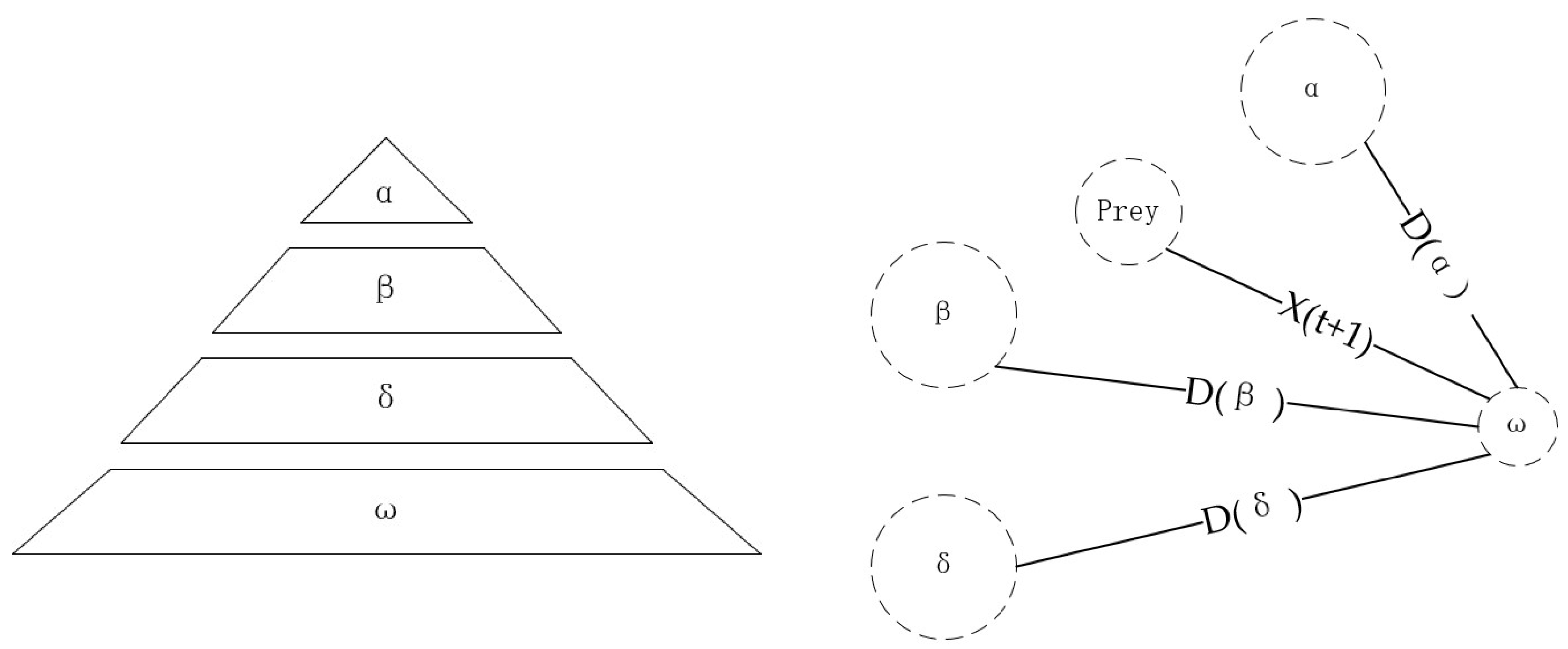
The GWO algorithm was proposed by Seyedali et al. in 2014, inspired by the cooperative hunting of grey wolves’ hierarchy [11]. At the very beginning, the GWO algorithm will generate initial wolves in a particular domain. Similarly, each wolf presents a solution which will be evaluated by the algorithm in each generation [12]. In that case, the three best solutions will be chosen as the leaders of the wolves to guide others in approaching the prey. In the optimization process, the prey represents the real solution, while the nearest wolf is the global optimum. These SI algorithms provide new methods to data exploration in both engineering and science [13,14,15,16,17,18]. Compared with other algorithms, GWO has a simple structure and high convergence speed. However, it also has disadvantages. For example, it can easily fall into local optimum. Therefore, many improved GWO algorithms have been proposed [19,20,21,22,23,24,25].

Li et al. proposed a new method combining improved grey wolf optimization (IGWO) and kernel extreme learning machine (KELM). This method combines the genetic algorithm (GA) and grey wolf optimization to generate discrete populations, and then obtain the optimal solution through KELM [26]. Long et al. introduced a MAL-IGWO algorithm, which integrates both the searching capability of improved grey wolf optimization (IGWO) and the capability of modified augmented Lagrangian (MAL) in solving constrained problems [27]. Gao et al. represented an improved grey wolf optimization algorithm (VW-GWO) based on variable weights, in which the searching process obeys the social hierarchy at the same time [28].

To enhance the performance of algorithm, learning strategies were also adopted to the algorithms. For instance, the opposition-based learning (OBL) strategy is widely accepted for its superior convergence ability. The OBL operates by generating numbers in an opposite interval. Moreover, some variants of OBL have been also proposed. For instance, a quasi-opposite number is applied to broaden the domain which is named original idea of quasi-opposite-based learning (QOBL). Moreover, a quasi-reflection based learning (QRBL) strategy is adopted by introducing a quasi-reflection number in the interval of the current position and the center position.

Besides the above GWO algorithm variants, an improved GWO based on a dynamic opposite learning strategy is introduced in this paper. It is named as dynamic opposite learning-assisted grey wolf optimizer (DOLGWO). In the first section, the background of optimization algorithms is introduced; then the GWO algorithm and dynamic opposite learning strategy are shown in the second section; the DOLGWO algorithm is given in the third section; in the fourth section all nine algorithms are compared to prove the superior performance of DOLGWO; and the conclusion is made in the fifth section at last.

2. Algorithm Preliminaries

2.1. GWO Algorithm

As a type of population-based meta-heuristics, Swarm Intelligence (SI) algorithms were originated from natural animals, such as colonies, ants. PSO, ACO and many other popular SI algorithms are widely applied in real world. Among these algorithms, the grey wolf optimization algorithm is a superior method to tackle numerical problems. In [29], GWO algorithm is compared with BBO, LI, HM, CS, ABC, ABCNN, QP and GAMS. The results show that the GWO algorithm is able to provide very competitive results compared to these well-known meta-heuristics. In [30], empirical studies are conducted to compare GWO algorithm with different metaheuristics such as LSHADE, TLBO and EBO with CMAR, NDHS, BA, CLPSO, EAD, RPSO, CDE, NCDE and LIPS. Experimental results show that the GWO algorithm performs better than the other algorithms on most benchmarks and engineering problems. In [31], the GWO algorithm is compared to GA, PSOGSA and gradient-based algorithm. Results from both synthetic and real data demonstrate that GWO algorithm can show a good balance between exploration and exploitation. In [11], the GWO algorithm provided highly competitive results compared to well-known heuristics such as PSO, GSA, DE, EP and ES. Due to its accuracy calculation and the smaller population assigned in global and local searching procedures, the GWO algorithm converges faster and even easier than others [32,33,34].

GWO algorithm was inspired by the behaviors and the social hierarchy of the wolves. According to wolves’ social hierarchy, there are four groups which are $\alpha$, $\beta$, $\delta$ and $\omega$ respectively, as shown in Figure 1. The $\alpha$ is the fittest solution which can guide others to go towards the right direction, $\beta$ and $\delta$ are the second and third best solution respectively. Moreover, the $\omega$ is the basement, which provides a large amount of population to support the whole pack.

When searching a prey, the iteration begins (t = 1) and three coefficients A, C and D are introduced to describe the encircling model, as follows:

$$D=C·X_P\left(t\right)-X\left(t\right)$$

(1)

$$X(t+1)=X_p\left(t\right)-A·D$$

(2)

$$A=2\mathrm{a}·r_1-\mathrm{a}$$

(3)

$$C=2r_2$$

(4)

$$a=2(1-\frac{t}{t_{max}})$$

(5)

where t indicates the current iteration; $X\left(t\right)$ is the position vector of the wolf; $X_p\left(t\right)$ is the position of the prey; A is the rand vector; C is the adaptive vector; D is the distance vector between the prey and wolf; $r_1$ and $r_2$ are both rand vectors in [0,1]; a is the convergence factor which goes down linearly from 2 to 0.

The hunting process is shown as follows:

$$D_{\partial }=C_1·X_{\partial }\left(\mathrm{t}\right)-X$$

(6)

$$D_{\beta }=C_2·X_{\beta }\left(\mathrm{t}\right)-X$$

(7)

$$D_{\delta }=C_3·X_{\delta }\left(\mathrm{t}\right)-X$$

(8)

$$X\left(1\right)=X_{\partial }\left(\mathrm{t}\right)-A_1·D_{\partial }$$

(9)

$$X\left(2\right)=X_{\beta }\left(\mathrm{t}\right)-A_2·D_{\beta }$$

(10)

$$X\left(3\right)=X_{\delta }\left(\mathrm{t}\right)-A_3·D_{\delta }$$

(11)

$$X(t+1)=\frac{(X_1+X_2+X_3)}{3}$$

(12)

Generally, when |A| < 1 $\omega$ wolves will move away from the prey and explore wider space for a global optimal value. On contrary, when |A| > 1 $\omega$ wolves will move closer to the prey which means local dominants in optimization.

2.2. Opposition-Based Learning (OBL)

The optimization algorithms aim to generate solutions, optimize estimated solutions and search for more solutions in the domain. When solving a complex problem, the existing solutions cannot meet the requirements. In that case, many learning strategies are created to enhance the performance of optimization algorithms. Among these learning strategies, the opposition-based learning (OBL) strategy is widely accepted for its superior convergence ability. The definition of OBL is introduced as follows:

The OBL consists of $X\in R$ which is a real number in a certain interval: $X\in [a,b]$. In addition, the opposite number $X^O$ is generated.

$$X^O=\mathrm{a}+\mathrm{b}-X$$

(13)

when it comes to a multi-dimentional situation, the definition is showed as follows:

Assuming that $X=(X_1,X_2,\dots ,X_D)$ is a point in D dimensional coordinates with $X_1,X_2,\dots ,X_D\in R$ in the interval of $[a_{\mathrm{j}},b_{\mathrm{j}}]$. With the changing of iteration, $a_j$, $b_j$ are the corresponding low and high boundaries of the population, respectively. Meanwhile, the multi-dimensional opposite point is defined as:

$$X_j^O=a_j+b_j-X_j$$

(14)

although the OBL strategy improve the searching ability of algorithm, it still has some disadvantages, such as premature. To improve the performance of OBL, some variants of OBL have been proposed. For instance, a quasi-opposite number is applied to broaden the domain which is named original idea of quasi-opposite based learning (QOBL) [34]. Meanwhile, a quasi-reflection-based learning (QRBL) strategy is adopted by introducing a quasi-reflection number in the interval of the current position and the center position [35].

2.3. Dynamic Opposite Learning Phase

Besides the above variants of OBL, a new learning strategy named dynamic opposite learning operator (DOL) is adopted in this paper. The DOL strategy was first proposed by Xu et al. to improve the performance of TLBO algorithm in [36]. The DOL is introduced to keep the algorithm away from prematurity when meeting complicated problems [37]. Moreover, the DOL learning strategy is a new variant of opposition-based learning (OBL) strategy, which helps the population learn from the opposite points in an asymmetric and dynamic search space [33,38].

In the initialization step, $X\in [a,b]$ were defined as the initial population. Moreover, $X^O$ is generated in the opposite domain. In order to enlarge the searching space, $X^{RO}$ ($X^{RO}=\mathrm{rand}·X^O,rand\in [0,1]$) is introduced to replace $X^O$ to change the former symmetric searching space into a dynamic asymmetric domain. In that case, the optimizer is able to enlarge the searching space, which can avoid the prematurity. Therefore, a weighting factor w is introduced to improve the ability to overcome local optima. The mathematical model is shown as follows:

$$X^{DO}=X+w·r_2·(r_1·X^{\mathrm{O}}-\mathrm{X})$$

(15)

where $r_2$ is a random parameter, $r_2\in [0,1]$. Confronted with a multi-dimension objective, it shows as follows:

$$X_j^{DO}=X_j+w·r_2·\left(r_1·X_j^O-X_j\right)$$

(16)

where $X=(X_1,X_2,...,X_D)\in [a_j,b_j]$ is the individuals in a D-dimensional space; The $a_j$ and $b_j$ are the boundaries of $X_j$. $X_j^{DO}$ is the $j\mathrm{th}$ dimension’s dynamic opposite point.

The population will be updated with iteration. If the fitness values were better, X will be replaced by $X^{DO}$. On contrary, the X will be retained and recorded in the new population. The new fitness value should be in the range of $[a_j,b_j]$, or it will be reset as a random in the domain.

3. DOL-Based GWO Optimization Algorithm

In this section, a novel DOL-based GWO algorithm is proposed, and both the learning strategy and algorithm steps are represented. The DOL strategy is separated into two parts: one is population and parameter initialization, the other is generating new solutions by updating operations. To update the population, a jumping rate (Jr) is adopted in DOL, while weighting factor w is a positive factor that aims to balance the exploration and exploitation capability. As long as the selection probability is smaller than Jr, the DOL operation process can be implemented as follows:

$${P_{ij}}^{DO}=P_{ij}+w·ran{d}_1·[ran{d}_2·(a_j+b_j-P_{ij})-P_{ij}]$$

(17)

where a random value $P_{ij}$ is generated as the initial population; $P_{ij}^{DO}$ is the population generated by DOL strategy; Np is the population size; i is the $i\mathrm{th}$ solution; j presents the $j\mathrm{th}$ dimension; $ran{d}_1$ and $ran{d}_2$ are two random parameters in [0,1]; weighting factor w is set as 8; jumping rate is set as 0.3.

With the updating of population, the boundaries are changed in the same way,

$$a_j=min\left(P_{ij}\right),b_j=max\left(P_{ij}\right)$$

(18)

The individuals are selected in the range of $[a_j,b_j]$ which is composed by $P_{ij}$ and $P_{ij}^{DO}$.

DOLGWO Algorithm Steps

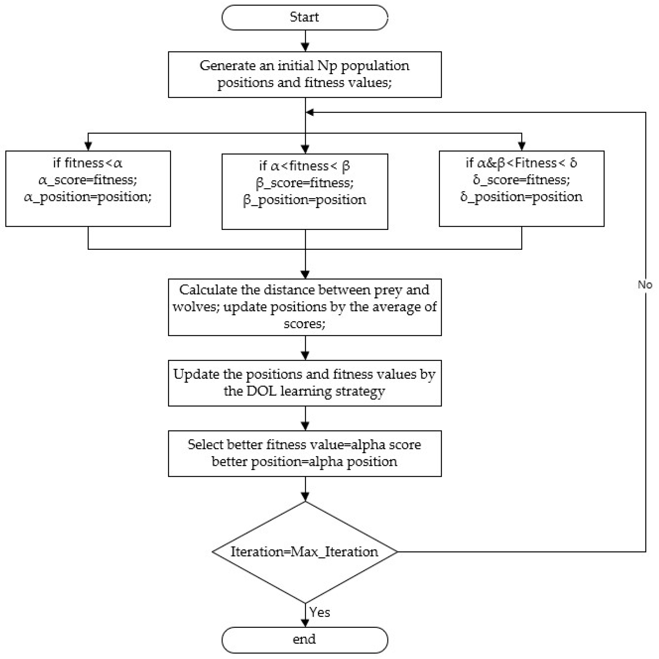
In this section, a new variant of GWO algorithm is introduced which is named as DOLGWO algorithm, as illustrated in Algorithm 1. The flowchart visualization of the algorithm is also shown in Figure 2.

Algorithm 1 The DOLGWO Algorithm

Randomly generate an initial population P and Alpha, Beta, Delta position;

while G ≤ maximal evolutionary iteration do

for $i=1;i\le Np;i++$ do

Generate “fitness” value to evaluate all learners by the fitness function f(.)

end for

for $i=1;i\le Np;i++$ do

Check boundaries

if fitness < Alpha score then

Update Alpha’s position and score

end if

if fitness(i) > Alpha_score $\&\&$ fitness(i) < Beta_score then

Update Beta’s position and score

end if

if fitness(i) > Alpha_score $\&\&$ fitness(i) > Beta_score $\&\&$ fitness(i) < Delta_score then

Update Delta’s position and score

end if

end for

for $i=1;i\le Np;i++$ do

for $j=1;j\le D;j++$ do

Update the population P

end for

end for

if rand < Jr then

for $i=1;i\le Np;i++$ do

${\mathrm{r}}_{1i}$ = rand(0, 1), ${\mathrm{r}}_{2\mathrm{i}}$ = rand(0, 1);

for $j=1;j\le D;j++$ do

${\mathrm{a}}_{\mathrm{j}}$ = min($P_{\mathrm{ij}}$), ${\mathrm{b}}_{\mathrm{j}}$ = max($P{}_{\mathrm{ij}}$);

${P_{ij}}^{DO}=P_{ij}+w·r{l}_i·[r{2}_i·(a_j+b_j-P_{ij})-P_{ij}]$

Check boundaries

end for

end for

for j = 1: Np do

Evaluate the fitness values of the new individuals ${\mathrm{fitness}}^{DO}$;

end for

for $i=1;i\le Np;i++$ do

if ${\mathrm{fitness}}^{DO}$(i) < fitness(i) then

Update Population P

end if

end for

Sort the fitness value;

if ${\mathrm{fitness}}^{DO}$ < Alpha score then

Update alpha position

end if

end if

Update the P, and the fitness value is assigned to best score;

G++

end while

4. Experiment and Discussion

4.1. Benchmark Function

In this section, 23 different benchmark functions which contains unimodal problems, multi-modal problems and hybrid problems are applied to test the performance of DOLGWO as shown in

Table 1. Benchmark functions provided by CEC2014 test set.

Label	Function	Optimum	Dims	Character
F1	High Conditioned Elliptic	100	30	Unimodal
F2	Bent Cigar	200	30	Unimodal
F3	Discus	300	30	Unimodal
F4	Rosenbrock	400	30	Multimodal
F5	Ackley	500	30	Multimodal
F6	Weierstrass	600	30	Multimodal
F7	Griewank	700	30	Multimodal
F8	Rastrigin	800	30	Multimodal
F9	Rotated Rastrigin	900	30	Multimodal
F10	Schwefel	1000	30	Multimodal
F11	Rotated Schwefel	1100	30	Multimodal
F12	Katsuura	1200	30	Multimodal
F13	HappyCat	1300	30	Multimodal
F14	HGBat	1400	30	Multimodal
F15	Expanded Griewank’s plus Rosenbrock	1500	30	Multimodal
F16	Expanded Scaffer	1600	30	Multimodal
F17	HF1	1700	30	Hybrid
F18	HF2	1800	30	Hybrid
F19	HF3	1900	30	Hybrid
F20	HF4	2000	30	Hybrid
F21	HF5	2100	30	Hybrid
F22	HF6	2200	30	Hybrid
F23	CF1	2300	30	Composition

. In this paper, all the benchmark functions are provided by CEC2014 test set and they are effective to verify its performance. Three unimodal functions are adopted to test the DOLGWO’s exploitation since it has only one global optimal solution and no local optimum in the searching domain. While multi-modal functions can obtain plenty of local optimums, which means the exploration capability can be examined. For closer inspection, both hybrid functions and composition functions are conducted to examine its performance.

4.2. Parameter Settings

Numerical experiments include five different algorithms, consisting of the grey wolf optimization algorithm (GWO), teaching learning optimization algorithm (TLBO), pigeon-inspired optimization algorithm (PIO) and Jaya optimization algorithm. The parameter settings are listed in

Table 2. Parameter settings of optimization algorithms.

Parameters	Value
Size of population	100
Total generation number for test functions	2500
Times conducting the experiment	3
Jr of DOLGWO	0.3
w of DOLGWO	8
Map and compass factor of PIO	0.2

and they are explained in detail. In the PIO algorithm, the map and compass factor R is set as 0.2; in the DOLGWO algorithm, the weighting factor w and jumping rate Jr are set as 8 and 0.3.

The parameters’ settings are crucial to the algorithm’s performance, especially for DOLGWO. In that case, the sensitivity analysis of the parameters is implemented in this section. As shown in

Table 3. The sensitivity analysis of w.

Weight	Mean				Std				Best
	F3	F6	F18	F23	F3	F6	F18	F23	Num
1	$1.93\times {10}^6$	$-5.67\times {10}^2$	$3.90\times {10}^8$	$-1.90\times {10}^3$	$5.22\times {10}^7$	$4.93\times {10}^2$	$1.48\times {10}^9$	$1.81\times {10}^3$	0
2	$5.76\times {10}^7$	$5.71\times {10}^2$	$2.61\times {10}^9$	$-1.77\times {10}^3$	$5.76\times {10}^7$	$4.95\times {10}^2$	$2.12\times {10}^9$	$1.89\times {10}^3$	0
3	$3.19\times {10}^5$	$-5.67\times {10}^2$	$4.99\times {10}^8$	$-1.74\times {10}^3$	$2.65\times {10}^6$	$4.92\times {10}^2$	$1.94\times {10}^9$	$1.89\times {10}^3$	0
4	$5.89\times {10}^5$	$-5.70\times {10}^2$	$7.81\times {10}^8$	$-1.73\times {10}^3$	$7.77\times {10}^6$	$4.89\times {10}^2$	$2.06\times {10}^9$	$1.91\times {10}^3$	0
5	$1.11\times {10}^6$	$-5.66\times {10}^2$	$1.88\times {10}^9$	$-1.79\times {10}^3$	$1.50\times {10}^7$	$4.92\times {10}^2$	$2.57\times {10}^9$	$1.95\times {10}^3$	0
6	$2.42\times {10}^6$	$-5.65\times {10}^2$	$4.20\times {10}^8$	$-1.81\times {10}^3$	$4.20\times {10}^7$	$4.89\times {10}^2$	$1.82\times {10}^9$	$1.91\times {10}^3$	0
7	$2.55\times {10}^6$	$-5.66\times {10}^2$	$1.06\times {10}^9$	$-1.77\times {10}^3$	$4.00\times {10}^7$	$4.95\times {10}^2$	$2.05\times {10}^9$	$1.88\times {10}^3$	0
8	$1.42\times {10}^5$	$-5.44\times {10}^2$	$5.94\times {10}^8$	$-1.64\times {10}^3$	$1.23\times {10}^6$	$4.83\times {10}^2$	$1.98\times {10}^9$	$1.70\times {10}^3$	3
9	$6.59\times {10}^5$	$-5.64\times {10}^2$	$3.71\times {10}^8$	$-1.79\times {10}^3$	$9.71\times {10}^6$	$4.90\times {10}^2$	$1.35\times {10}^9$	$1.91\times {10}^3$	1
10	$3.55\times {10}^5$	$-5.68\times {10}^2$	$4.24\times {10}^8$	$-1.74\times {10}^3$	$7.07\times {10}^6$	$4.89\times {10}^2$	$1.75\times {10}^9$	$1.79\times {10}^3$	0

and

Table 4. The sensitivity analysis of Jr.

Jr	Mean				Std				Best
	F3	F6	F18	F23	F3	F6	F18	F23	Num
0.1	$1.75\times {10}^5$	$-5.66\times {10}^2$	$4.52\times {10}^8$	$-1.75\times {10}^3$	$7.58\times {10}^5$	$4.90\times {10}^2$	$1.90\times {10}^9$	$1.89\times {10}^3$	0
0.2	$5.52\times {10}^5$	$-5.66\times {10}^2$	$1.75\times {10}^9$	$-1.86\times {10}^3$	$7.78\times {10}^6$	$4.91\times {10}^2$	$2.54\times {10}^9$	$1.91\times {10}^3$	0
0.3	$1.42\times {10}^5$	$-5.44\times {10}^2$	$3.64\times {10}^8$	$-1.64\times {10}^3$	$1.23\times {10}^6$	$4.83\times {10}^2$	$1.54\times {10}^9$	$1.70\times {10}^3$	3
0.4	$3.70\times {10}^5$	$-5.70\times {10}^2$	$3.70\times {10}^8$	$-1.78\times {10}^3$	$5.19\times {10}^6$	$4.90\times {10}^2$	$1.80\times {10}^9$	$1.89\times {10}^3$	0
0.5	$1.42\times {10}^6$	$-5.69\times {10}^2$	$1.09\times {10}^9$	$-1.73\times {10}^3$	$2.54\times {10}^7$	$4.90\times {10}^2$	$1.87\times {10}^9$	$1.94\times {10}^3$	1
0.6	$1.34\times {10}^6$	$-5.70\times {10}^2$	$4.69\times {10}^8$	$-1.60\times {10}^3$	$1.64\times {10}^7$	$4.91\times {10}^2$	$1.99\times {10}^9$	$1.97\times {10}^3$	0
0.7	$2.30\times {10}^6$	$-5.70\times {10}^2$	$3.76\times {10}^8$	$-1.74\times {10}^3$	$6.36\times {10}^7$	$4.90\times {10}^2$	$1.89\times {10}^9$	$1.91\times {10}^3$	0
0.8	$3.59\times {10}^5$	$-5.66\times {10}^2$	$6.30\times {10}^8$	$-1.77\times {10}^3$	$4.59\times {10}^6$	$4.97\times {10}^2$	$2.12\times {10}^9$	$1.98\times {10}^3$	0
0.9	$1.95\times {10}^5$	$-5.67\times {10}^2$	$5.64\times {10}^8$	$-1.90\times {10}^3$	$1.47\times {10}^6$	$4.93\times {10}^2$	$1.98\times {10}^9$	$1.94\times {10}^3$	0
1	$4.92\times {10}^5$	$-5.68\times {10}^2$	$4.38\times {10}^8$	$-1.89\times {10}^3$	$8.49\times {10}^6$	$4.90\times {10}^2$	$1.64\times {10}^9$	$1.83\times {10}^3$	0

, test functions are selected for analysis. Where, F3 is unimodal function, F6 is multi-modal function, F18 is hybrid function and F23 is composition function. The mean and standard deviation of the results gained by DOLGWO are also recorded to evaluate the performance in the Table 3 and Table 4. When Jr = 0.3, DOLGWO performs better than other settings in F3, F6 and F18 respectively. When w = 8, it shows predominant results in F3, F6, F23. As a result, w = 8, Jr = 0.3 is the most suitable parameters setting.

Moreover, the population number for all test is 100, while the FES is set as 100*2500. All the experiments are implemented three times.

4.3. Unimodal/Multi-Modal Test Functions and Their Analysis

Table 5. The mean and standard value of unimodal/multi-modal test functions.

Algorithms	F1		F2		F3		F4
	Mean	Std	Mean	Std	Mean	Std	Mean	Std
DOLGWO	$5.43\times {10}^8$	$5.07\times {10}^8$	$5.15\times {10}^{10}$	$1.73\times {10}^{10}$	$1.42\times {10}^5$	$1.23\times {10}^6$	$1.30\times {10}^4$	$8.98\times {10}^3$
GWO	$6.07\times {10}^8$	$3.74\times {10}^8$	$5.16\times {10}^{10}$	$1.47\times {10}^{10}$	$1.43\times {10}^5$	$1.17\times {10}^6$	$6.89\times {10}^3$	$6.03\times {10}^3$
TLBO	$6.17\times {10}^9$	$2.77\times {10}^9$	$1.49\times {10}^{11}$	$7.65\times {10}^9$	$1.43\times {10}^5$	$2.46\times {10}^6$	$5.42\times {10}^4$	$9.73\times {10}^3$
PIO	$2.20\times {10}^9$	$4.35\times {10}^8$	$1.45\times {10}^{11}$	$1.23\times {10}^{10}$	$1.43\times {10}^5$	$4.74\times {10}^4$	$3.79\times {10}^4$	$4.25\times {10}^3$
Jaya	$1.78\times {10}^9$	$9.92\times {10}^8$	$1.09\times {10}^{11}$	$1.89\times {10}^{10}$	$1.43\times {10}^5$	$9.40\times {10}^5$	$2.72\times {10}^4$	$6.20\times {10}^3$
Algorithms	F5		F6		F7		F8
	Mean	Std	Mean	Std	Mean	Std	Mean	Std
DOLGWO	$-4.78\times {10}^2$	$4.08\times {10}^2$	$-5.44\times {10}^2$	$4.83\times {10}^2$	$-4.31\times {10}^2$	$6.29\times {10}^2$	$-5.43\times {10}^2$	$6.50\times {10}^2$
GWO	$-4.79\times {10}^2$	$4.08\times {10}^2$	$-5.49\times {10}^2$	$4.92\times {10}^2$	$-4.93\times {10}^2$	$6.04\times {10}^2$	$-5.65\times {10}^2$	$6.51\times {10}^2$
TLBO	$-4.79\times {10}^2$	$4.07\times {10}^2$	$-5.27\times {10}^2$	$4.93\times {10}^2$	$-8.47\times {10}^0$	$5.54\times {10}^2$	$-4.87\times {10}^2$	$6.63\times {10}^2$
PIO	$-4.79\times {10}^2$	$4.09\times {10}^2$	$-5.24\times {10}^2$	$4.95\times {10}^2$	$-1.00\times {10}^1$	$5.18\times {10}^2$	$-4.43\times {10}^2$	$6.64\times {10}^2$
Jaya	$-4.79\times {10}^2$	$4.08\times {10}^2$	$-5.37\times {10}^2$	$4.89\times {10}^2$	$-3.45\times {10}^2$	$5.46\times {10}^2$	$-4.94\times {10}^2$	$6.61\times {10}^2$
Algorithms	F9		F10		F11		F12
	Mean	Std	Mean	Std	Mean	Std	Mean	Std
DOLGWO	$-6.43\times {10}^2$	$7.52\times {10}^2$	$7.67\times {10}^3$	$1.93\times {10}^3$	$1.06\times {10}^4$	$2.68\times {10}^3$	$-1.19\times {10}^3$	$9.80\times {10}^2$
GWO	$-6.07\times {10}^2$	$7.48\times {10}^2$	$8.29\times {10}^3$	$2.26\times {10}^3$	$1.12\times {10}^4$	$2.54\times {10}^3$	$-1.20\times {10}^3$	$9.79\times {10}^2$
TLBO	$-5.25\times {10}^2$	$7.25\times {10}^2$	$1.32\times {10}^4$	$1.12\times {10}^3$	$1.33\times {10}^4$	$9.31\times {10}^2$	$-1.20\times {10}^3$	$9.80\times {10}^2$
PIO	$-5.19\times {10}^2$	$7.40\times {10}^2$	$1.17\times {10}^4$	$5.10\times {10}^2$	$1.35\times {10}^4$	$1.06\times {10}^3$	$-1.20\times {10}^3$	$9.79\times {10}^2$
Jaya	$-5.16\times {10}^2$	$7.39\times {10}^2$	$1.03\times {10}^4$	$2.38\times {10}^3$	$1.29\times {10}^4$	$1.36\times {10}^3$	$-1.20\times {10}^3$	$9.80\times {10}^2$
Algorithms	F13		F14		F15		F16
	Mean	Std	Mean	Std	Mean	Std	Mean	Std
DOLGWO	$-1.30\times {10}^3$	$1.05\times {10}^3$	$-1.28\times {10}^3$	$1.14\times {10}^3$	$7.57\times {10}^5$	$1.57\times {10}^7$	$-1.57\times {10}^3$	$1.31\times {10}^3$
GWO	$-1.30\times {10}^3$	$1.06\times {10}^3$	$-1.29\times {10}^3$	$1.16\times {10}^3$	$1.90\times {10}^5$	$5.26\times {10}^6$	$-1.58\times {10}^3$	$1.31\times {10}^3$
TLBO	$-1.29\times {10}^3$	$1.06\times {10}^3$	$-1.00\times {10}^3$	$1.15\times {10}^3$	$5.83\times {10}^6$	$1.22\times {10}^7$	$-1.58\times {10}^3$	$1.30\times {10}^3$
PIO	$-1.28\times {10}^3$	$1.06\times {10}^3$	$-1.02\times {10}^3$	$1.15\times {10}^3$	$5.88\times {10}^6$	$3.75\times {10}^6$	$-1.58\times {10}^3$	$1.31\times {10}^3$
Jaya	$-1.29\times {10}^3$	$1.06\times {10}^3$	$-1.22\times {10}^3$	$1.18\times {10}^3$	$4.47\times {10}^6$	$6.59\times {10}^6$	$-1.58\times {10}^3$	$1.31\times {10}^3$
Algorithms	DOLGWO	GWO	TLBO	PIO	Jaya
Best num	8	2	2	3	1

shows the mean and standard deviation values of five algorithms on 16 unimodal/multi-modal functions. F1–F3 are unimodal functions. The results present that DOLGWO performs better than other algorithms on all three unimodal functions. Further, it can be concluded that the DOL strategy with expending search spaces are more likely to reach the global optimum for its exploitation capability.

F4–F16 functions are multi-modal functions which are applied to verify the exploration capability of DOLGWO. Compared with other algorithms, the results in Table 5 show that DOLGWO performs well, especially on F5, F10, F11, F12 and F16 test functions.

4.4. Analysis of Hybrid Test Functions and Composition Functions

To imitate the practical problems, hybrid functions are conducted to test the algorithms through combining unimodal and multi-modal functions. To deal with hybrid functions, it is necessary to balance exploitation and exploration capability which may result in poor performance. In

Table 6. The mean and standard value of hybrid and composition test functions.

Algorithms	F17		F18		F19		F20
	Mean	Std	Mean	Std	Mean	Std	Mean	Std
DOLGWO	$1.04\times {10}^8$	$1.18\times {10}^8$	$3.64\times {10}^8$	$1.54\times {10}^9$	$-1.53\times {10}^3$	$1.46\times {10}^3$	$8.62\times {10}^5$	$3.38\times {10}^7$
GWO	$4.97\times {10}^7$	$9.24\times {10}^7$	$1.75\times {10}^9$	$1.77\times {10}^9$	$-1.51\times {10}^3$	$1.53\times {10}^3$	$2.48\times {10}^5$	$1.24\times {10}^7$
TLBO	$1.16\times {10}^8$	$7.48\times {10}^7$	$2.04\times {10}^{10}$	$6.59\times {10}^9$	$2.72\times {10}^1$	$1.97\times {10}^3$	$2.27\times {10}^5$	$9.87\times {10}^6$
PIO	$6.76\times {10}^7$	$5.08\times {10}^7$	$8.18\times {10}^9$	$2.58\times {10}^9$	$-2.19\times {10}^2$	$1.01\times {10}^3$	$1.40\times {10}^6$	$9.73\times {10}^5$
Jaya	$3.43\times {10}^7$	$9.35\times {10}^7$	$8.26\times {10}^9$	$3.59\times {10}^9$	$-1.37\times {10}^3$	$1.47\times {10}^3$	$2.79\times {10}^5$	$4.64\times {10}^6$
Algorithms	F21		F22		F23		Best num
	Mean	Std	Mean	Std	Mean	Std	Mean	Std
DOLGWO	$1.04\times {10}^7$	$3.15\times {10}^7$	$4.80\times {10}^2$	$1.53\times {10}^4$	$-1.64\times {10}^3$	$1.70\times {10}^3$	3	2
GWO	$1.09\times {10}^7$	$2.96\times {10}^7$	$2.60\times {10}^3$	$5.34\times {10}^4$	$-1.62\times {10}^3$	$1.90\times {10}^3$	0	0
TLBO	$7.70\times {10}^7$	$6.81\times {10}^7$	$1.12\times {10}^4$	$1.09\times {10}^5$	$-2.09\times {10}^3$	$1.88\times {10}^3$	2	0
PIO	$2.70\times {10}^7$	$1.63\times {10}^7$	$8.90\times {10}^3$	$1.47\times {10}^4$	$-1.13\times {10}^3$	$1.90\times {10}^3$	1	0
Jaya	$1.26\times {10}^7$	$3.12\times {10}^7$	$6.20\times {10}^3$	$1.82\times {10}^5$	$-1.21\times {10}^3$	$1.78\times {10}^3$	1	5

, the advantages of DOLGWO can be easily found on F18, F21, F22 and the composition function shows that DOLGWO can still solve it no worse than other algorithms. In that case, the DOLGWO can balance the convergence speed and optimization solution well in many practical problems.

4.5. Statistical Test Results

T test is applied to figure out difference between the average value of two independent samples. T values are showed in

Table 7. The T values of DOLGWO and other algorithms.

Algorithms	DOLGWO
	F1	F2	F3	F4	F5	F6	F7	F8
GWO	$5.56\times {10}^1$	$2.41\times {10}^{-2}$	$3.22\times {10}^{-3}$	$3.09\times {10}^0$	$9.49\times {10}^{-3}$	$3.97\times {10}^{-1}$	$3.83\times {10}^{-1}$	$1.31\times {10}^{-1}$
TLBO	$1.09\times {10}^1$	$2.82\times {10}^1$	$1.99\times {10}^{-3}$	$1.70\times {10}^1$	$9.50\times {10}^{-3}$	$1.35\times {10}^{-1}$	$2.76\times {10}^0$	$3.30\times {10}^{-1}$
PIO	$1.78\times {10}^0$	$2.41\times {10}^1$	$4.45\times {10}^{-3}$	$1.37\times {10}^1$	$9.48\times {10}^{-3}$	$1.58\times {10}^{-1}$	$2.83\times {10}^0$	$5.89\times {10}^{-1}$
Jaya	$1.31\times {10}^0$	$1.23\times {10}^0$	$3.54\times {10}^{-3}$	$7.13\times {10}^0$	$9.49\times {10}^{-3}$	$5.58\times {10}^{-2}$	$5.66\times {10}^{-1}$	$2.89\times {10}^{-1}$
Algorithms	DOLGWO
	F9	F10	F11	F12	F13	F14	F15	F16
GWO	$1.86\times {10}^{-1}$	$1.14\times {10}^0$	$8.90\times {10}^{-1}$	$3.95\times {10}^{-2}$	0	$3.37\times {10}^{-2}$	$1.88\times {10}^{-1}$	$2.96\times {10}^{-2}$
TLBO	$6.19\times {10}^{-1}$	$1.36\times {10}^1$	$5.21\times {10}^0$	$3.95\times {10}^{-2}$	0	$9.47\times {10}^{-1}$	$-1.40\times {10}^0$	$2.96\times {10}^{-2}$
PIO	$6.44\times {10}^{-1}$	$1.11\times {10}^1$	$5.51\times {10}^0$	$3.95\times {10}^{-2}$	$7.34\times {10}^{-2}$	$8.79\times {10}^{-1}$	$-1.74\times {10}^0$	$2.96\times {10}^{-2}$
Jaya	$6.59\times {10}^{-1}$	$4.70\times {10}^0$	$4.19\times {10}^0$	$3.95\times {10}^{-2}$	0	$2.00\times {10}^{-1}$	$-1.19\times {10}^0$	$2.96\times {10}^{-2}$
Algorithms	DOLGWO
	F17	F18	F19	F20	F21	F22	F23
GWO	$1.98\times {10}^0$	$-3.24\times {10}^0$	$-5.18\times {10}^{-2}$	$9.34\times {10}^{-2}$	$-6.34\times {10}^{-2}$	$-2.09\times {10}^{-1}$	$-4.30\times {10}^{-2}$
TLBO	$-4.70\times {10}^{-1}$	$-1.62\times {10}^1$	$-3.48\times {10}^0$	$9.88\times {10}^{-2}$	$-4.86\times {10}^0$	$-5.33\times {10}^{-1}$	$9.72\times {10}^{-1}$
PIO	$1.55\times {10}^0$	$-1.42\times {10}^1$	$-4.04\times {10}^0$	$-8.71\times {10}^{-2}$	$-2.56\times {10}^0$	$-2.17\times {10}^0$	$-1.10\times {10}^0$
Jaya	$2.54\times {10}^0$	$-1.11\times {10}^1$	$-4.23\times {10}^{-1}$	$9.36\times {10}^{-2}$	$-2.72\times {10}^{-1}$	$-1.72\times {10}^{-1}$	$-9.57\times {10}^{-1}$

. P values are represented in

Table 8. The P values of DOLGWO and other algorithms.

Algorithms	DOLGWO
	F1	F2	F3	F4	F5	F6	F7	F8
GWO	-	-	-	+	-	-	-	-
TLBO	+	+	-	+	-	-	+	-
PIO	-	+	-	+	-	-	+	-
Jaya	-	-	-	+	-	-	-	-
Algorithms	DOLGWO
	F9	F10	F11	F12	F13	F14	F15	F16
GWO	-	-	-	-	-	-	-	-
TLBO	-	+	+	-	-	-	-	-
PIO	-	+	+	-	-	-	-	-
Jaya	-	+	+	-	-	-	-	-
Algorithms	DOLGWO
	F17	F18	F19	F20	F21	F22	F23	P < 0.05
GWO	-	+	-	-	-	-	-	21
TLBO	-	+	+	-	+	-	-	14
PIO	-	+	+	-	+	+	-	14
Jaya	+	+	-	-	-	-	-	18

, which is marked as +, −. The value of 0.05 is set as the level of significance, t (30)0.05 = 2.0423. When the value t < 2.0423, it indicates P > 0.05. In that case, the null hypothesis is eligible, which means that no significant difference exists between two algorithms. On the contrary, null hypotheses are rejected; these algorithms are significantly different.

From Table 8, the results show that DOLGWO mostly performs significantly differently to other algorithms.

4.6. Analysis of Convergence

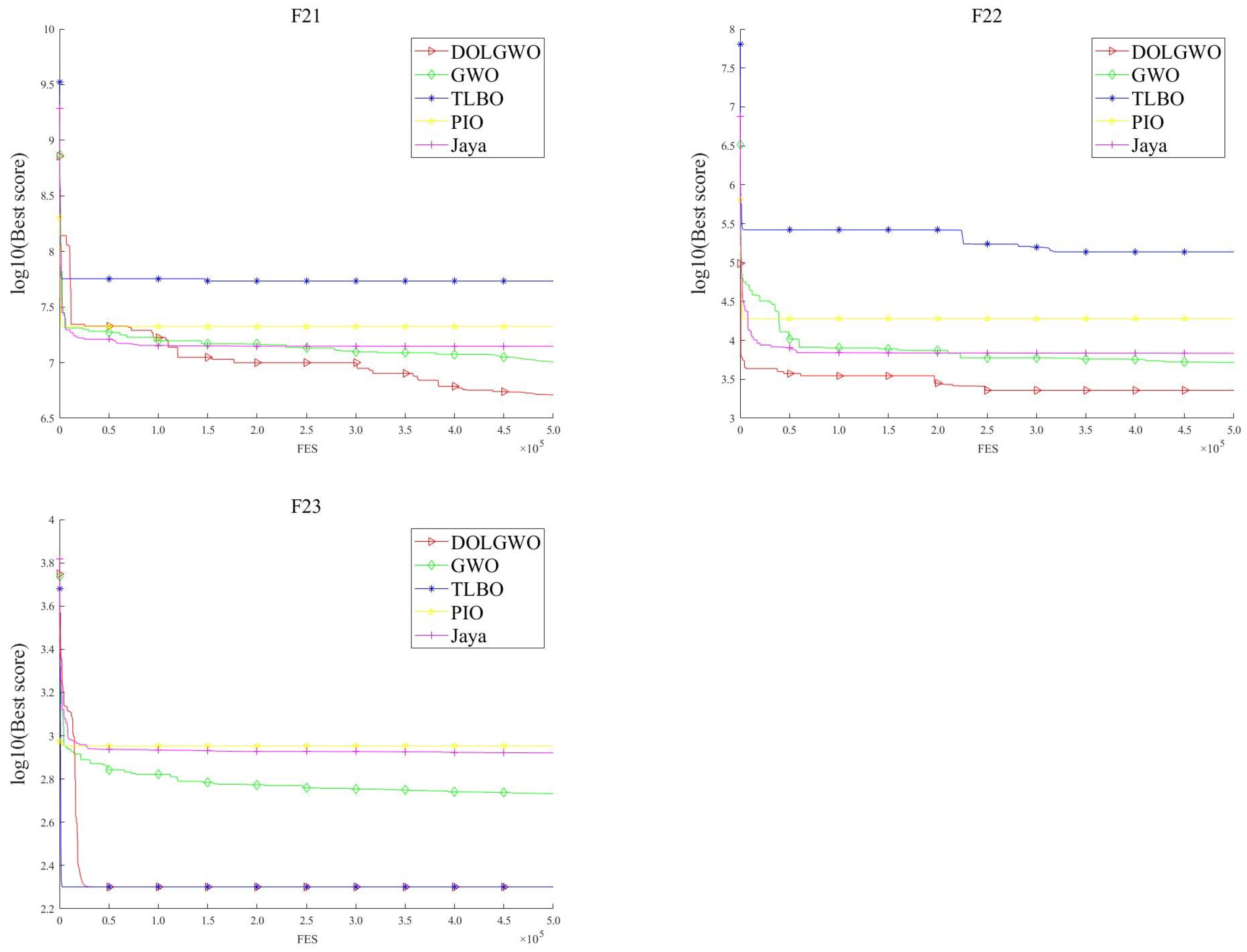
The convergence capability of five algorithms on test functions are plotted in Figure 3, where the ‘Best score’ presents the average of fitness value. As the figures show, DOLGWO converges fast along with the iterative computing, which results from the remarkable exploration capability. As for the gradually converging trend, it is due to the exploitation capability of the DOL strategy.

4.7. Repeat the Experiment and Compare with the Improved Algorithms

To prove the superiority of DOLGWO, a number of alternative improved meta-heuristic algorithms are selected for comparison purposes, including several variants of particle swarm optimization (CFPSO and CFWPSO), several variants of teacher–learning-based optimization (ETLBO, CTLBO and NTLBO) and grey wolf Optimization (GWO). The parameter details of DOLGWO are as follows: weighting factor w and jumping rate Jr are set as 8 and 0.3, which are the same as the previous experiment.

The parameter settings of the other improved meta-heuristic algorithms were selected as follows. In cfPSO and cfwPSO, the cognitive and social acceleration coefficients (C1 and C2) are set as 2.05 with the constriction factor K = 0.729. The population size is 30 in all cases. For all 23 benchmark functions, function evaluations (FES) is 50 × 10,000. The mean and standard deviation (Std) of the objective function f(X) averaged over three repetitions of the algorithms are recorded for each benchmark function, while the best numbers of mean and standard deviation are recorded for all improved meta-heuristic algorithms in

Table 9. The mean and standard value of 23 test functions.

Algorithms	F1		F2		F3		F4
	Mean	Std	Mean	Std	Mean	Std	Mean	Std
DOLGWO	$1.49\times {10}^8$	$1.67\times {10}^8$	$1.95\times {10}^{10}$	$5.24\times {10}^9$	$5.69\times {10}^4$	$1.39\times {10}^4$	$2.13\times {10}^3$	$5.83\times {10}^2$
GWO	$1.76\times {10}^8$	$1.36\times {10}^8$	$2.41\times {10}^{10}$	$1.55\times {10}^{10}$	$6.68\times {10}^4$	$1.88\times {10}^4$	$2.46\times {10}^3$	$2.26\times {10}^2$
CFPSO	$5.32\times {10}^8$	$2.19\times {10}^8$	$6.97\times {10}^{10}$	$8.68\times {10}^9$	$9.63\times {10}^4$	$1.46\times {10}^4$	$1.65\times {10}^4$	$1.88\times {10}^3$
CFWPSO	$7.37\times {10}^9$	$1.21\times {10}^8$	$6.57\times {10}^{10}$	$8.88\times {10}^9$	$1.04\times {10}^5$	$5.44\times {10}^3$	$1.39\times {10}^4$	$3.51\times {10}^3$
ETLBO	$1.78\times {10}^9$	$7.34\times {10}^8$	$1.30\times {10}^{11}$	$2.62\times {10}^{10}$	$1.52\times {10}^5$	$1.46\times {10}^4$	$3.36\times {10}^4$	$6.82\times {10}^3$
CTLBO	$1.42\times {10}^9$	$2.27\times {10}^8$	$9.46\times {10}^{10}$	$4.08\times {10}^9$	$1.21\times {10}^5$	$1.46\times {10}^4$	$2.16\times {10}^4$	$6.10\times {10}^3$
NTLBO	$1.95\times {10}^9$	$3.49\times {10}^8$	$1.22\times {10}^{11}$	$1.15\times {10}^{10}$	$1.41\times {10}^5$	$3.86\times {10}^4$	$3.06\times {10}^4$	$4.64\times {10}^3$
Algorithms	F5		F6		F7		F8
	Mean	Std	Mean	Std	Mean	Std	Mean	Std
DOLGWO	$5.21\times {10}^2$	$2.77\times {10}^{-2}$	$6.35\times {10}^2$	$1.96\times {10}^0$	$8.49\times {10}^2$	$9.19\times {10}^1$	$1.05\times {10}^3$	$4.12\times {10}^1$
GWO	$5.21\times {10}^2$	$6.36\times {10}^{-2}$	$6.33\times {10}^2$	$2.18\times {10}^0$	$8.55\times {10}^2$	$3.31\times {10}^1$	$1.05\times {10}^3$	$2.14\times {10}^1$
CFPSO	$5.21\times {10}^2$	$9.82\times {10}^{-2}$	$6.56\times {10}^2$	$4.67\times {10}^0$	$1.37\times {10}^3$	$2.09\times {10}^2$	$1.21\times {10}^3$	$2.23\times {10}^1$
CFWPSO	$5.21\times {10}^2$	$2.37\times {10}^{-2}$	$6.56\times {10}^2$	$5.67\times {10}^0$	$1.34\times {10}^3$	$1.02\times {10}^2$	$1.20\times {10}^3$	$3.65\times {10}^1$
ETLBO	$5.21\times {10}^2$	$9.34\times {10}^{-2}$	$6.70\times {10}^2$	$3.09\times {10}^{-1}$	$1.90\times {10}^3$	$2.26\times {10}^2$	$1.38\times {10}^3$	$3.00\times {10}^0$
CTLBO	$5.21\times {10}^2$	$1.79\times {10}^{-2}$	$6.61\times {10}^2$	$3.90\times {10}^0$	$1.56\times {10}^3$	$1.47\times {10}^2$	$1.24\times {10}^3$	$4.43\times {10}^1$
NTLBO	$5.21\times {10}^2$	$5.18\times {10}^{-2}$	$6.66\times {10}^2$	$1.03\times {10}^0$	$1.79\times {10}^3$	$1.85\times {10}^2$	$1.32\times {10}^3$	$2.20\times {10}^1$
Algorithms	F9		F10		F11		F12
	Mean	Std	Mean	Std	Mean	Std	Mean	Std
DOLGWO	$1.11\times {10}^3$	$1.73\times {10}^1$	$7.54\times {10}^3$	$6.79\times {10}^2$	$9.42\times {10}^3$	$4.11\times {10}^3$	$1.20\times {10}^3$	$2.13\times {10}^0$
GWO	$1.14\times {10}^3$	$2.87\times {10}^1$	$6.89\times {10}^3$	$1.27\times {10}^2$	$7.70\times {10}^3$	$1.58\times {10}^3$	$1.20\times {10}^3$	$2.02\times {10}^0$
CFPSO	$1.33\times {10}^3$	$4.92\times {10}^1$	$9.56\times {10}^3$	$2.25\times {10}^2$	$1.01\times {10}^4$	$1.66\times {10}^3$	$1.20\times {10}^3$	$4.09\times {10}^{-1}$
CFWPSO	$1.39\times {10}^3$	$3.38\times {10}^1$	$8.65\times {10}^3$	$8.86\times {10}^2$	$1.18\times {10}^4$	$1.09\times {10}^3$	$1.20\times {10}^3$	$2.79\times {10}^{-1}$
ETLBO	$1.58\times {10}^3$	$5.39\times {10}^1$	$1.50\times {10}^4$	$7.65\times {10}^2$	$1.52\times {10}^4$	$1.75\times {10}^3$	$1.20\times {10}^3$	$4.44\times {10}^{-1}$
CTLBO	$1.40\times {10}^3$	$5.95\times {10}^1$	$1.10\times {10}^4$	$4.03\times {10}^2$	$1.21\times {10}^4$	$1.01\times {10}^3$	$1.20\times {10}^3$	$2.21\times {10}^{-1}$
NTLBO	$1.51\times {10}^3$	$6.40\times {10}^1$	$1.33\times {10}^4$	$9.90\times {10}^2$	$1.37\times {10}^4$	$1.31\times {10}^2$	$1.20\times {10}^3$	$2.90\times {10}^{-1}$
Algorithms	F13		F14		F15		F16
	Mean	Std	Mean	Std	Mean	Std	Mean	Std
DOLGWO	$1.30\times {10}^3$	$1.76\times {10}^0$	$1.44\times {10}^3$	$5.87\times {10}^0$	$4.02\times {10}^3$	$1.04\times {10}^3$	$1.62\times {10}^3$	$1.08\times {10}^0$
GWO	$1.30\times {10}^3$	$9.06\times {10}^{-2}$	$1.44\times {10}^3$	$1.05\times {10}^0$	$6.86\times {10}^3$	$6.56\times {10}^3$	$1.62\times {10}^3$	$5.24\times {10}^{-1}$
CFPSO	$1.31\times {10}^3$	$3.16\times {10}^{-1}$	$1.56\times {10}^3$	$4.68\times {10}^0$	$7.77\times {10}^5$	$7.12\times {10}^5$	$1.62\times {10}^3$	$4.49\times {10}^{-1}$
CFWPSO	$1.31\times {10}^3$	$3.16\times {10}^{-1}$	$1.56\times {10}^3$	$4.68\times {10}^0$	$7.77\times {10}^5$	$7.12\times {10}^5$	$1.62\times {10}^3$	$5.36\times {10}^{-1}$
ETLBO	$1.31\times {10}^3$	$8.04\times {10}^{-1}$	$1.69\times {10}^3$	$2.39\times {10}^1$	$1.75\times {10}^6$	$8.14\times {10}^5$	$1.62\times {10}^3$	$7.63\times {10}^{-1}$
CTLBO	$1.31\times {10}^3$	$7.31\times {10}^{-1}$	$1.60\times {10}^3$	$1.70\times {10}^1$	$6.07\times {10}^5$	$2.51\times {10}^5$	$1.62\times {10}^3$	$4.89\times {10}^{-1}$
NTLBO	$1.31\times {10}^3$	$7.00\times {10}^{-2}$	$1.74\times {10}^3$	$4.64\times {10}^1$	$1.76\times {10}^6$	$6.78\times {10}^5$	$1.62\times {10}^3$	$3.69\times {10}^{-1}$
Algorithms	F17		F18		F19		F20
	Mean	Std	Mean	Std	Mean	Std	Mean	Std
DOLGWO	$7.66\times {10}^6$	$5.03\times {10}^6$	$1.39\times {10}^8$	$1.37\times {10}^8$	$2.11\times {10}^3$	$1.09\times {10}^1$	$2.12\times {10}^4$	$1.20\times {10}^3$
GWO	$2.24\times {10}^7$	$1.81\times {10}^7$	$8.56\times {10}^7$	$1.48\times {10}^8$	$2.01\times {10}^3$	$5.54\times {10}^1$	$2.46\times {10}^4$	$1.05\times {10}^4$
CFPSO	$4.73\times {10}^7$	$4.10\times {10}^7$	$9.30\times {10}^8$	$4.12\times {10}^8$	$2.27\times {10}^3$	$1.01\times {10}^2$	$2.79\times {10}^4$	$1.39\times {10}^4$
CFWPSO	$7.51\times {10}^7$	$5.02\times {10}^7$	$2.11\times {10}^9$	$9.44\times {10}^8$	$2.38\times {10}^3$	$2.61\times {10}^2$	$2.91\times {10}^4$	$1.07\times {10}^4$
ETLBO	$1.96\times {10}^8$	$1.20\times {10}^8$	$7.60\times {10}^9$	$1.96\times {10}^9$	$3.09\times {10}^3$	$3.80\times {10}^2$	$1.07\times {10}^5$	$8.82\times {10}^4$
CTLBO	$1.66\times {10}^8$	$9.57\times {10}^7$	$3.60\times {10}^9$	$4.14\times {10}^8$	$2.44\times {10}^3$	$1.61\times {10}^2$	$4.38\times {10}^4$	$9.78\times {10}^3$
NTLBO	$2.74\times {10}^8$	$2.16\times {10}^8$	$8.23\times {10}^9$	$3.45\times {10}^9$	$2.69\times {10}^3$	$2.93\times {10}^2$	$6.41\times {10}^4$	$7.88\times {10}^3$
Algorithms	F21		F22		F23		Best num
	Mean	Std	Mean	Std	Mean	Std	Mean	Std
DOLGWO	$4.48\times {10}^6$	$6.22\times {10}^6$	$3.08\times {10}^3$	$3.39\times {10}^1$	$2.59\times {10}^3$	$1.63\times {10}^2$	12	7
GWO	$1.41\times {10}^6$	$1.64\times {10}^6$	$3.40\times {10}^3$	$2.93\times {10}^2$	$2.74\times {10}^3$	$3.81\times {10}^1$	8	5
CFPSO	$5.44\times {10}^6$	$4.53\times {10}^6$	$4.36\times {10}^3$	$2.66\times {10}^2$	$3.16\times {10}^3$	$2.12\times {10}^2$	2	0
CFWPSO	$9.25\times {10}^6$	$6.91\times {10}^6$	$5.20\times {10}^3$	$4.42\times {10}^2$	$3.08\times {10}^3$	$6.81\times {10}^1$	0	2
ETLBO	$2.97\times {10}^7$	$2.40\times {10}^9$	$9.10\times {10}^3$	$5.21\times {10}^3$	$2.50\times {10}^3$	$0.00\times {10}^0$	1	3
CTLBO	$1.16\times {10}^7$	$6.61\times {10}^6$	$1.19\times {10}^4$	$8.40\times {10}^3$	$2.92\times {10}^3$	$3.71\times {10}^2$	0	3
NTLBO	$3.16\times {10}^7$	$2.92\times {10}^7$	$1.09\times {10}^4$	$9.20\times {10}^3$	$2.50\times {10}^3$	$0.00\times {10}^0$	0	3

.

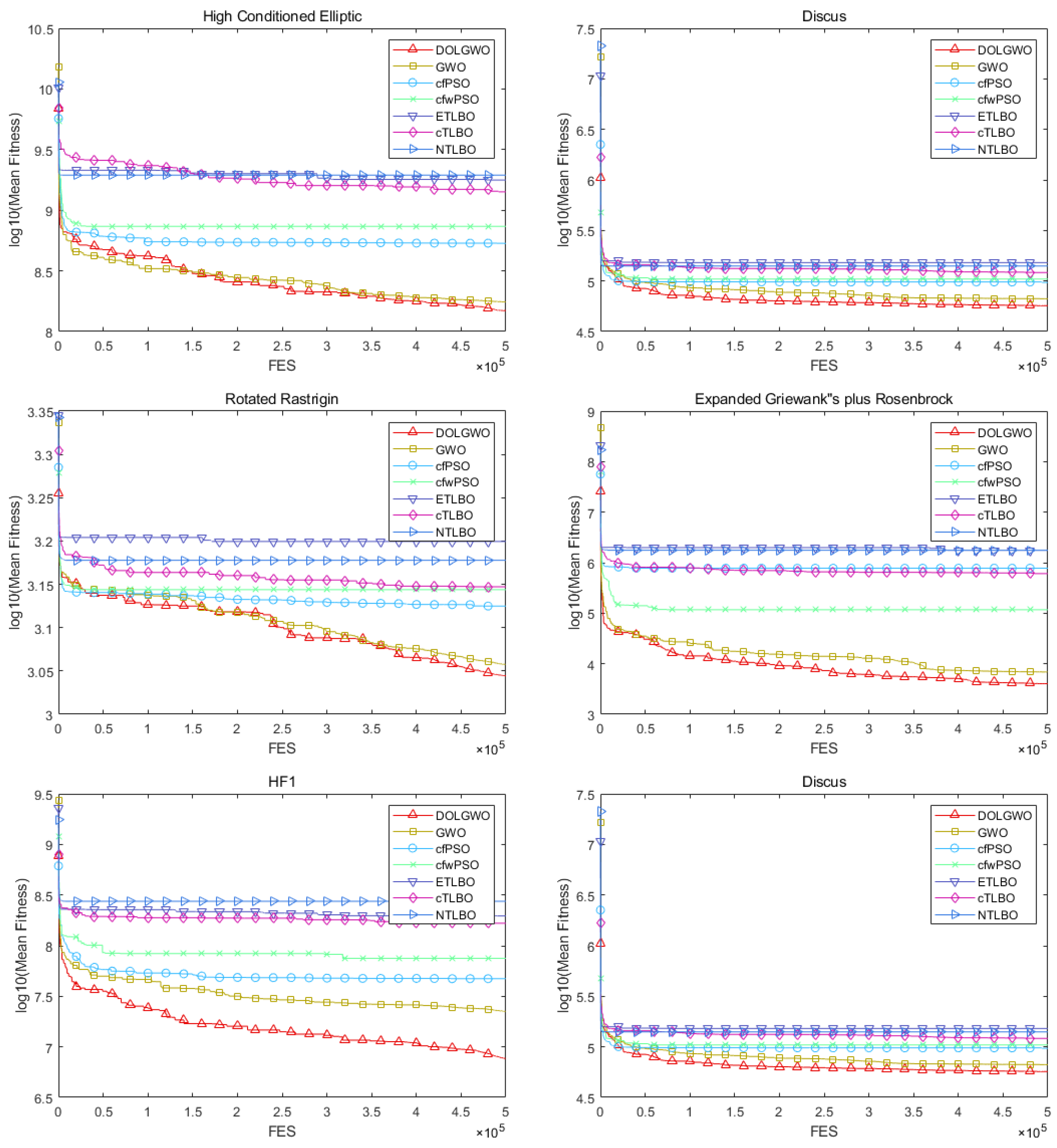
The results for all 23 benchmark functions are shown in Table 9, and the best average convergence results for 6 functions of DOLGWO are shown in Figure 4. It can be seen from these results that DOLGWO algorithm performs the best in all unimodal benchmark functions(3/3) and composition benchmark functions(1/1), in about half of multi-modal(6/13) and Hybrid benchmark functions(3/6).

DOLGWO algorithm is the best performing algorithm (Bust num Mean 12/23) and has the highest average standard deviation (Std) among all the improved algorithms considered in Table 9. In those results where DOLGWO is inferior to GWO, such as F5, F6, F8, F12 and F13, DOLGWO’s performance is very close to GWO. However, when the results of DOLGWO are better than those of GWO, the DOL strategy brings a big performance improvement, such as F1, F3, F9, F15, F17 and F22.

In most benchmark functions, DOLGWO achieves faster convergence early in computation and is faster than the GWO algorithm. DOLGWO continues to obtain better results when other algorithms do not change much. This shows that DOLGWO has strong robustness and adaptability. Hence, DOLGWO has the best performance among all compared algorithms, which demonstrates that the DOL strategy greatly improves the performance of the original GWO algorithm.

4.8. Repeat the Experiment and Compare with Other Improved DOL Algorithms

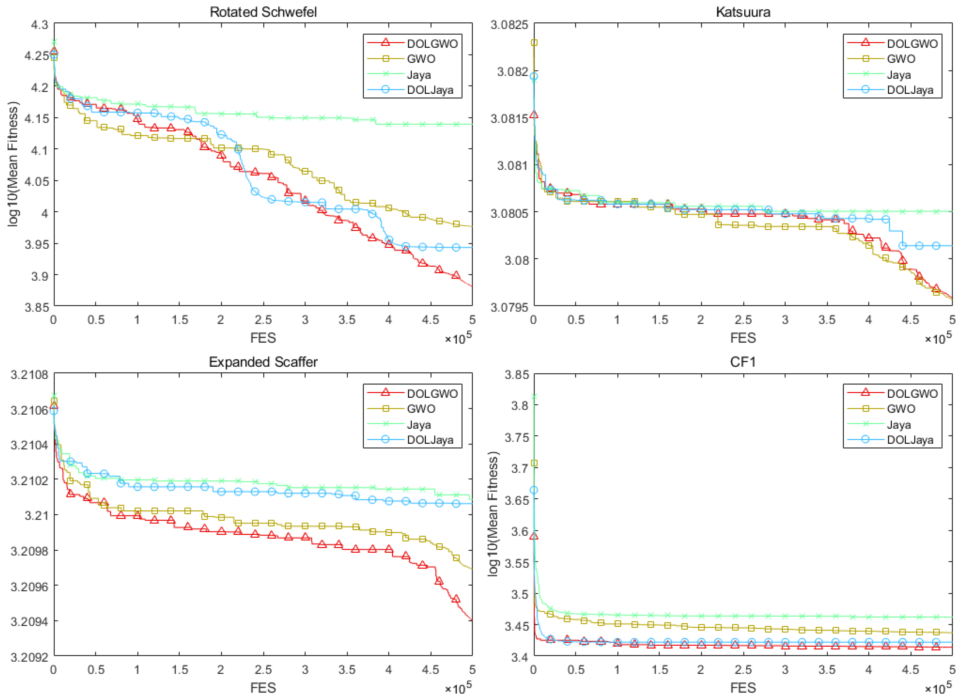
In order to illustrate the superiority of DOLGWO compared to other DOL-improved algorithms, numerical experiments are done on four algorithms including DOLGWO, DOLJaya, GWO and Jaya. The experimental conditions of DOLGWO are the same as the settings of the previous experiment, and the weighting factor w and jumping rate Jr of DOLJaya are set as 15 and 0.3, respectively.

The best average convergence results for four functions of DOLGWO are shown in Figure 5. It can be seen from the results that DOLJaya is better than Jaya and DOLGWO is significantly outperforming GWO, Jaya and DOLJaya. Among the DOL-improved algorithms, DOLGWO is more effective and advanced. It converges faster than DOLJaya and can continue to explore new solution spaces to obtain better solutions. Hence, we can conclude that incorporating the DOL strategy improves the performance of GWO and Jaya significantly. This is because DOLGWO and DOLJaya have a dynamic and asymmetric search space, which increases search exploitation and yields excellent convergence performance.

5. Conclusions

In this paper, a new DOLGWO algorithm has been proposed for solving complex optimization problems. It combines dynamic opposite learning strategy (DOL) with the GWO algorithm in order to improve convergence speed and robustness. The impacts of parameter setting and significance testing are also considered in the paper. The performance of DOLGWO is compared with 10 different algorithms, including 4 basic algorithms, 5 improved meta-heuristic algorithms and 1 improved DOL algorithm for 23 benchmark functions. The proposed DOLGWO algorithm mostly performs better than other participants. It converges faster and can continue to explore new solution spaces to obtain better solutions. This shows that DOLGWO has strong robustness and adaptability. Due to the dynamics and asymmetry characteristics of the DOL strategy, the convergence speed and searching exploitation of DOLGWO algorithm are obviously improved. In future work, DOLGWO algorithm will be applied to the actual short-term hydropower scheduling problem to further verify the performance of the algorithm.

References

1. Holland, J.H. Genetic algorithms and the optimal allocation of trials. SIAM J. Comput. 1973, 2, 88–105. [Google Scholar] [CrossRef]
2. Storn, R.; Price, K. Differential evolution–A simple and efficient heuristic for global optimization over continuous spaces. J. Glob. Optim. 1997, 11, 341–359. [Google Scholar] [CrossRef]
3. Sun, P.; Liu, H.; Zhang, Y.; Meng, Q.; Tu, L.; Zhao, J. An improved atom search optimization with dynamic opposite learning and heterogeneous comprehensive learning. Appl. Soft Comput. 2021, 103, 107140. [Google Scholar] [CrossRef]
4. Van, P.; Aarts, E. Simulated Annealing: Theory and Applications; Springer: Berlin/Heidelberg, Germany, 1987; pp. 7–15. [Google Scholar]
5. Rao, R.V.; Savsani, V.J.; Vakharia, D. Teaching–learning-based optimization: A novel method for constrained mechanical design optimization problems. Comput. Aided Des. 2011, 43, 303–315. [Google Scholar] [CrossRef]
6. Rao, R. Jaya: A simple and new optimization algorithm for solving constrained and unconstrained optimization problems. Int. J. Ind. Eng. Comput. 2016, 7, 19–34. [Google Scholar]
7. Kennedy, J.; Eberhart, R. Particle swarm optimization. In Proceedings of the ICNN’95 Iinternational Conference on Neural Networks, Perth, WA, Australia, 27 November–1 December 1995; Volume 4, pp. 1942–1948. [Google Scholar]
8. Karaboga, D.; Basturk, B. A powerful and efficient algorithm for numerical function optimization: Artificial bee colony (ABC) algorithm. J. Glob. Optim. 2007, 39, 459–471. [Google Scholar] [CrossRef]
9. Dorigo, M.; Stützle, T. Ant colony optimization: Overview and recent advances. Handbook of Metaheuristics; Springer: Berlin/Heidelberg, Germany, 2019; pp. 311–351. [Google Scholar]
10. Dong, H.; Xu, Y.; Li, X.; Yang, Z.; Zou, C. An improved antlion optimizer with dynamic random walk and dynamic opposite learning. Knowl. Based Syst. 2021, 216, 106752. [Google Scholar] [CrossRef]
11. Mirjalili, S.; Mirjalili, S.; Lewis, A. Grey Wolf Optimizer. Adv. Eng. Softw. 2014, 69, 46–61. [Google Scholar] [CrossRef]
12. Gao, Z.M.; Zhao, J.; Yang, Y.; Tian, X.J. The hybrid grey wolf optimization-slime mould algorithm. Proc. J. Phys. Conf. Ser. 2020, 1617, 012034. [Google Scholar] [CrossRef]
13. Saremi, S.; Mirjalili, S.Z.; Mirjalili, S.M. Evolutionary population dynamics and grey wolf optimizer. Neural Comput. Appl. 2015, 26, 1257–1263. [Google Scholar] [CrossRef]
14. Mirjalili, S.; Lewis, A. The whale optimization algorithm. Adv. Eng. Softw. 2016, 95, 51–67. [Google Scholar] [CrossRef]
15. Mirjalili, S. Moth-flame optimization algorithm: A novel nature-inspired heuristic paradigm. Knowl. Based Syst. 2015, 89, 228–249. [Google Scholar] [CrossRef]
16. Rao, R. Rao algorithms: Three metaphor-less simple algorithms for solving optimization problems. Int. J. Ind. Eng. Comput. 2020, 11, 107–130. [Google Scholar] [CrossRef]
17. Rao, R.V.; Saroj, A. Constrained economic optimization of shell-and-tube heat exchangers using elitist-Jaya algorithm. Energy 2017, 128, 785–800. [Google Scholar] [CrossRef]
18. Yu, K.; Liang, J.; Qu, B.; Chen, X.; Wang, H. Parameters identification of photovoltaic models using an improved JAYA optimization algorithm. Energy Convers. Manag. 2017, 150, 742–753. [Google Scholar] [CrossRef]
19. Heidari, A.A.; Pahlavani, P. An efficient modified grey wolf optimizer with Lévy flight for optimization tasks. Appl. Soft Comput. 2017, 60, 115–134. [Google Scholar] [CrossRef]
20. Muangkote, N.; Sunat, K.; Chiewchanwattana, S. An improved grey wolf optimizer for training q-Gaussian Radial Basis Functional-link nets. In Proceedings of the 2014 International Computer Science and Engineering Conference (ICSEC), Khon Kaen, Thailand, 30 July–1 August 2014; pp. 209–214. [Google Scholar]
21. Teeparthi, K.; Kumar, D.V. Grey wolf optimization algorithm based dynamic security constrained optimal power flow. In Proceedings of the 2016 National Power Systems Conference (NPSC), Bhubaneswar, India, 19–21 December 2016; pp. 1–6. [Google Scholar]
22. Yang, B.; Zhang, X.; Yu, T.; Shu, H.; Fang, Z. Grouped grey wolf optimizer for maximum power point tracking of doubly-fed induction generator based wind turbine. Energy Convers. Manag. 2017, 133, 427–443. [Google Scholar] [CrossRef]
23. Jayabarathi, T.; Raghunathan, T.; Adarsh, B.; Suganthan, P.N. Economic dispatch using hybrid grey wolf optimizer. Energy 2016, 111, 630–641. [Google Scholar] [CrossRef]
24. Amirsadri, S.; Mousavirad, S.J.; Ebrahimpour-Komleh, H. A Levy flight-based grey wolf optimizer combined with back-propagation algorithm for neural network training. Neural Comput. Appl. 2018, 30, 3707–3720. [Google Scholar] [CrossRef]
25. Oliveira, J.; Oliveira, P.M.; Boaventura-Cunha, J.; Pinho, T. Chaos-based grey wolf optimizer for higher order sliding mode position control of a robotic manipulator. Nonlinear Dyn. 2017, 90, 1353–1362. [Google Scholar] [CrossRef]
26. Li, Q.; Chen, H.; Huang, H.; Zhao, X.; Cai, Z.; Tong, C.; Liu, W.; Tian, X. An enhanced grey wolf optimization based feature selection wrapped kernel extreme learning machine for medical diagnosis. Comput. Math. Methods Med. 2017, 2017, 9512741. [Google Scholar] [CrossRef] [PubMed] [Green Version]
27. Long, W.; Liang, X.; Cai, S.; Jiao, J.; Zhang, W. A modified augmented Lagrangian with improved grey wolf optimization to constrained optimization problems. Neural Comput. Appl. 2017, 28, 421–438. [Google Scholar] [CrossRef]
28. Gao, Z.M.; Zhao, J. An improved grey wolf optimization algorithm with variable weights. Comput. Intell. Neurosci. 2019, 2019, 2981282. [Google Scholar] [CrossRef] [PubMed]
29. Wong, L.I.; Sulaiman, M.; Mohamed, M.; Hong, M.S. Grey Wolf Optimizer for solving economic dispatch problems. In Proceedings of the 2014 IEEE International Conference on Power and Energy (PECon), Kuching, Malaysia, 1–3 December 2014; pp. 150–154. [Google Scholar]
30. Lu, C.; Gao, L.; Yi, J. Grey wolf optimizer with cellular topological structure. Expert Syst. Appl. 2018, 107, 89–114. [Google Scholar] [CrossRef]
31. Song, X.; Tang, L.; Zhao, S.; Zhang, X.; Li, L.; Huang, J.; Cai, W. Grey wolf optimizer for parameter estimation in surface waves. Soil Dyn. Earthq. Eng. 2015, 75, 147–157. [Google Scholar] [CrossRef]
32. Faris, H.; Aljarah, I.; Al-Betar, M.A.; Mirjalili, S. Grey wolf optimizer: A review of recent variants and applications. Neural Comput. Appl. 2018, 30, 413–435. [Google Scholar] [CrossRef]
33. Liu, Z.H.; Wei, H.L.; Li, X.H.; Liu, K.; Zhong, Q.C. Global identification of electrical and mechanical parameters in PMSM drive based on dynamic self-learning PSO. IEEE Trans. Power Electron. 2018, 33, 10858–10871. [Google Scholar] [CrossRef]
34. Fu, Y.; Xiao, H.; Lee, L.H.; Huang, M. Stochastic optimization using grey wolf optimization with optimal computing budget allocation. Appl. Soft Comput. 2021, 103, 107154. [Google Scholar] [CrossRef]
35. Ergezer, M.; Simon, D.; Du, D. Oppositional biogeography-based optimization. In Proceedings of the 2009 IEEE International Conference on Systems, Man and Cybernetics, San Antonio, TX, USA, 11–14 October 2009; pp. 1009–1014. [Google Scholar]
36. Xu, Y.; Yang, Z.; Li, X.; Kang, H.; Yang, X. Dynamic opposite learning enhanced teaching–learning-based optimization. Knowl. Based Syst. 2020, 188, 104966. [Google Scholar] [CrossRef]
37. Zhou, J.; Zhang, Y.; Guo, Y.; Feng, W.; Menhas, M.; Zhang, Y. Parameters Identification of Battery Model Using a Novel Differential Evolution Algorithm Variant. Front. Energy Res. 2022, 10. [Google Scholar] [CrossRef]
38. Tizhoosh, H.R. Opposition-based learning: A new scheme for machine intelligence. In International Conference on Computational Intelligence for Modelling, Control and Automation and International Conference on Intelligent Agents, Web Technologies and Internet Commerce (CIMCA-IAWTIC 06); IEEE: Piscataway, NJ, USA, 2005; Volume 1, pp. 695–701. [Google Scholar]
Figure 1. Principle of GWO algorithm.
Symmetry 14 01871 g001
Figure 2. The flowchart of DOLGWO.
Symmetry 14 01871 g002
Figure 3. The convergence trends of all algorithms on 23 benchmark functions.
Symmetry 14 01871 g003aSymmetry 14 01871 g003bSymmetry 14 01871 g003c
Figure 4. The convergence trends of all algorithms on functions F1, F3, F9, F15, F17 and F22.
Symmetry 14 01871 g004
Figure 5. The convergence trends of four improved DOL algorithms on functions F11, F12, F16 and F23.
Symmetry 14 01871 g005