
Experimental and Numerical Studies of the Heat Transfer in Thin-Walled Rectangular Tubes under Fire

 ,
,  ,
, 
Abstract
:1. Introduction
- Model Law (ML), which includes the correlations of model behavior and prototype through dimensionless variables , and requires a skill obtained from previous applications;
- This protocol is non-unitary, requiring both deep knowledge in the field from the one who wants to apply it, and a certain ingenuity in separating and grouping the variables involved in describing the phenomenon in order to obtain the desired dimensionless variables;
- The protocol is not only difficult, but also precarious, because only in relatively simple cases does it allow us to obtain all the desired dimensionless variables (which would serve us to the complete description of the model–prototype correlation);
- The protocol also involves significant mathematical knowledge, which ensures the correct formulation of laws that describe as accurately as possible the pursued phenomenon (for example, heat transfer).
2. Materials and Methods
- Direct heating of the structural element covered with intumescent paint, i.e., when the thermal flux was applied from the outside to the protected element, resulting in , a value specified in the technical data sheet of the paint;
- Reverse heating, when the thermal flux was applied (through an electric current) from inside the structural element to the outside, thus obtaining , a difference of approximately 1%, which is highly acceptable considering the fact that these investigations did not have metrological conditions.
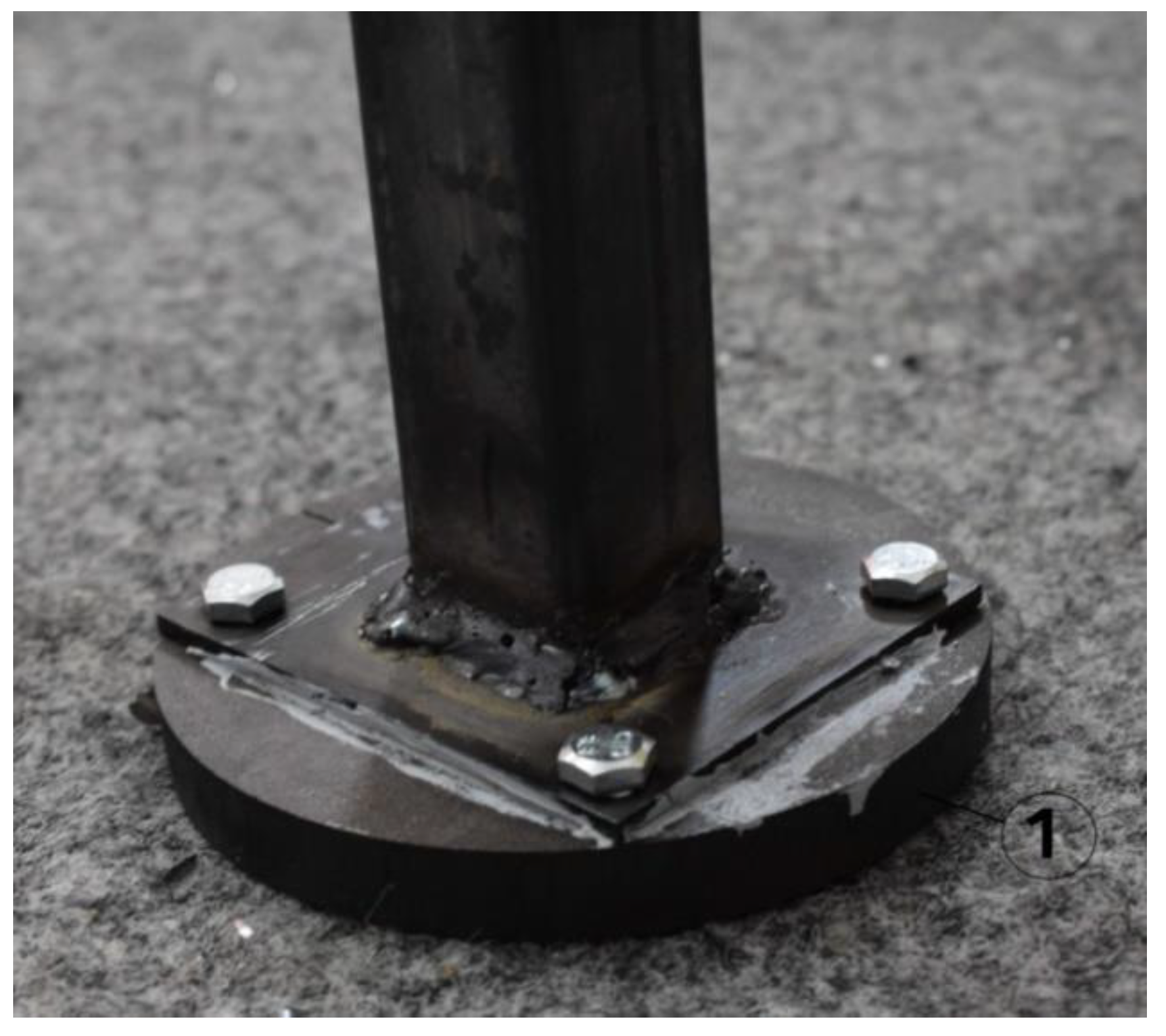
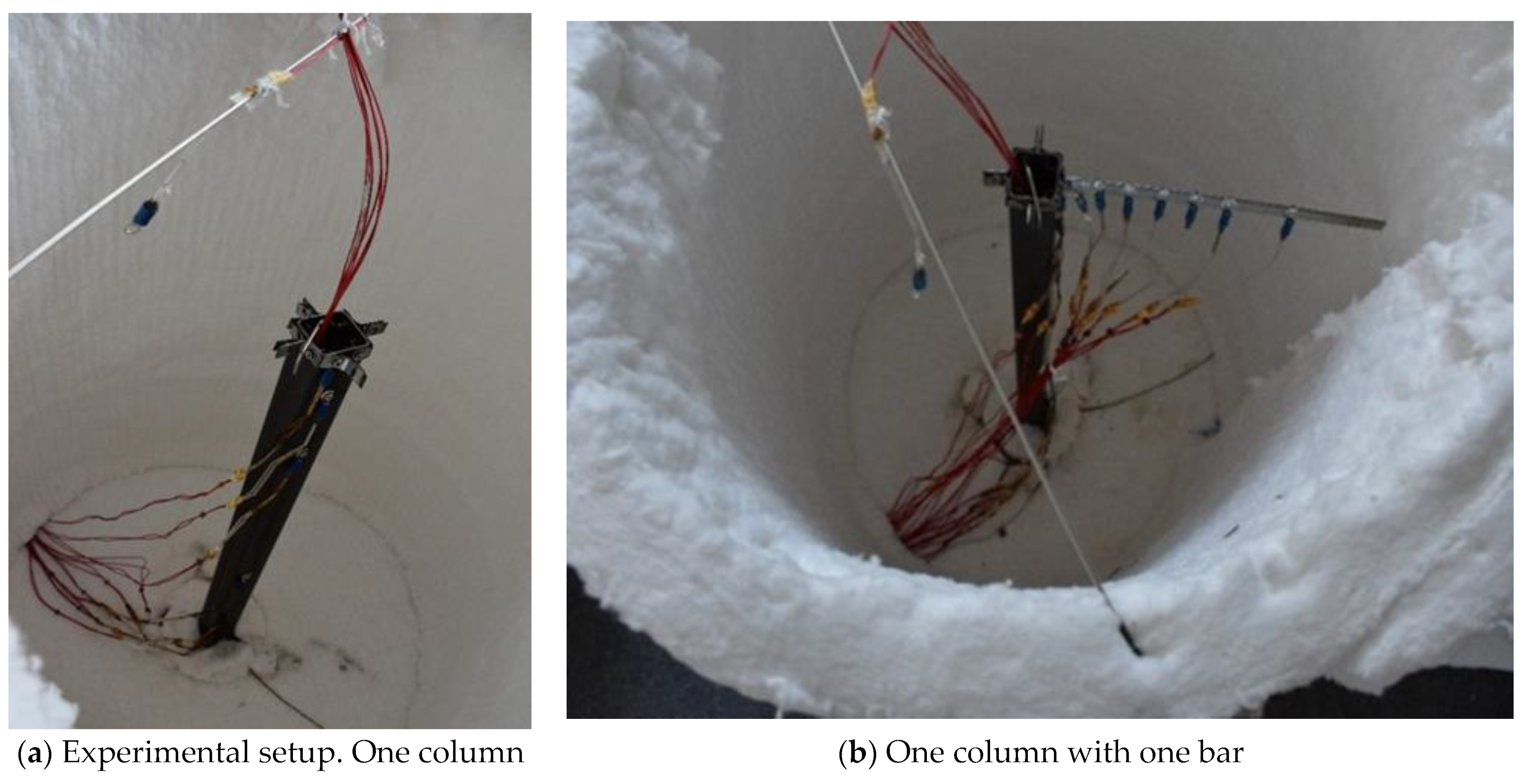
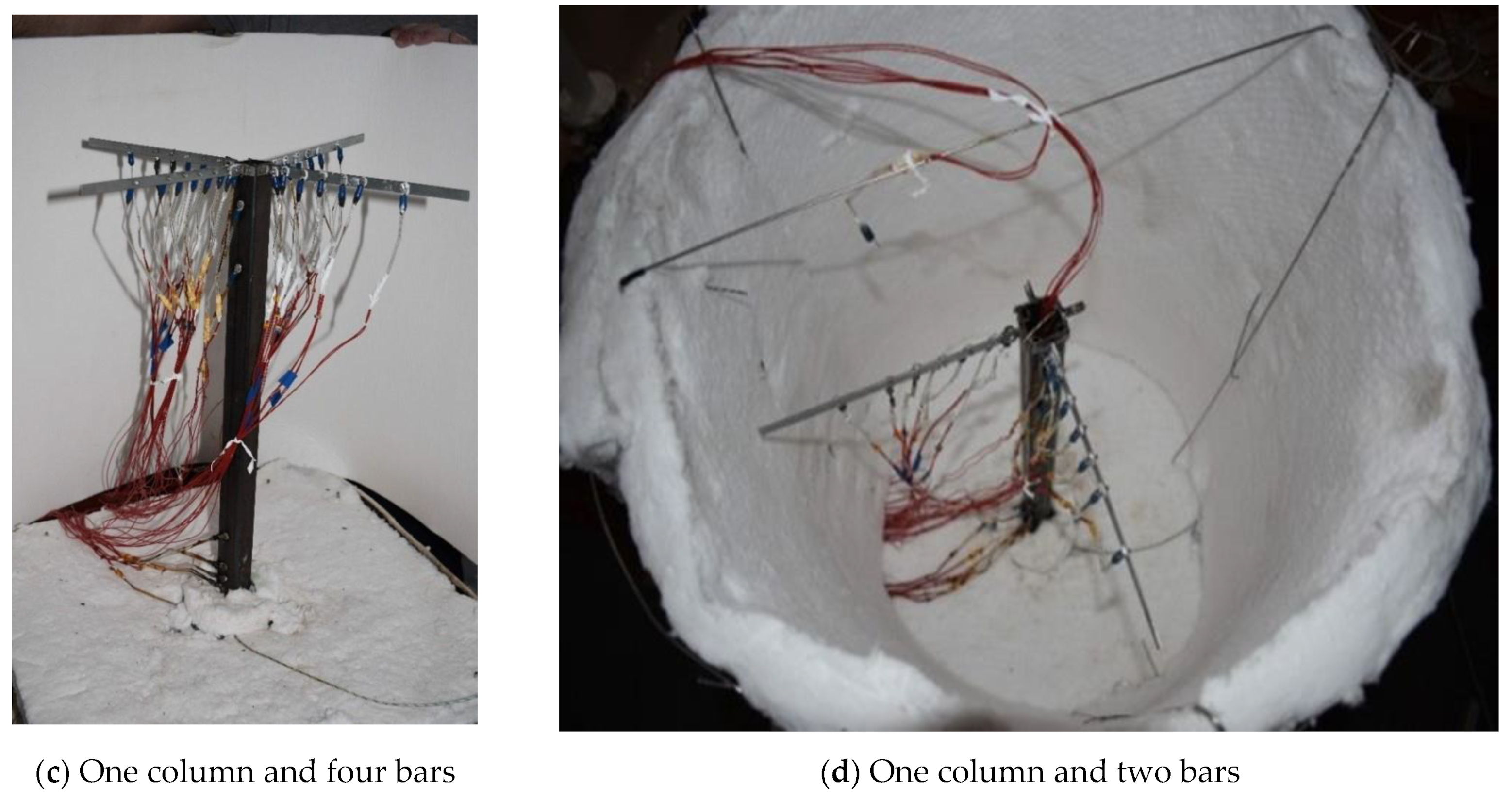
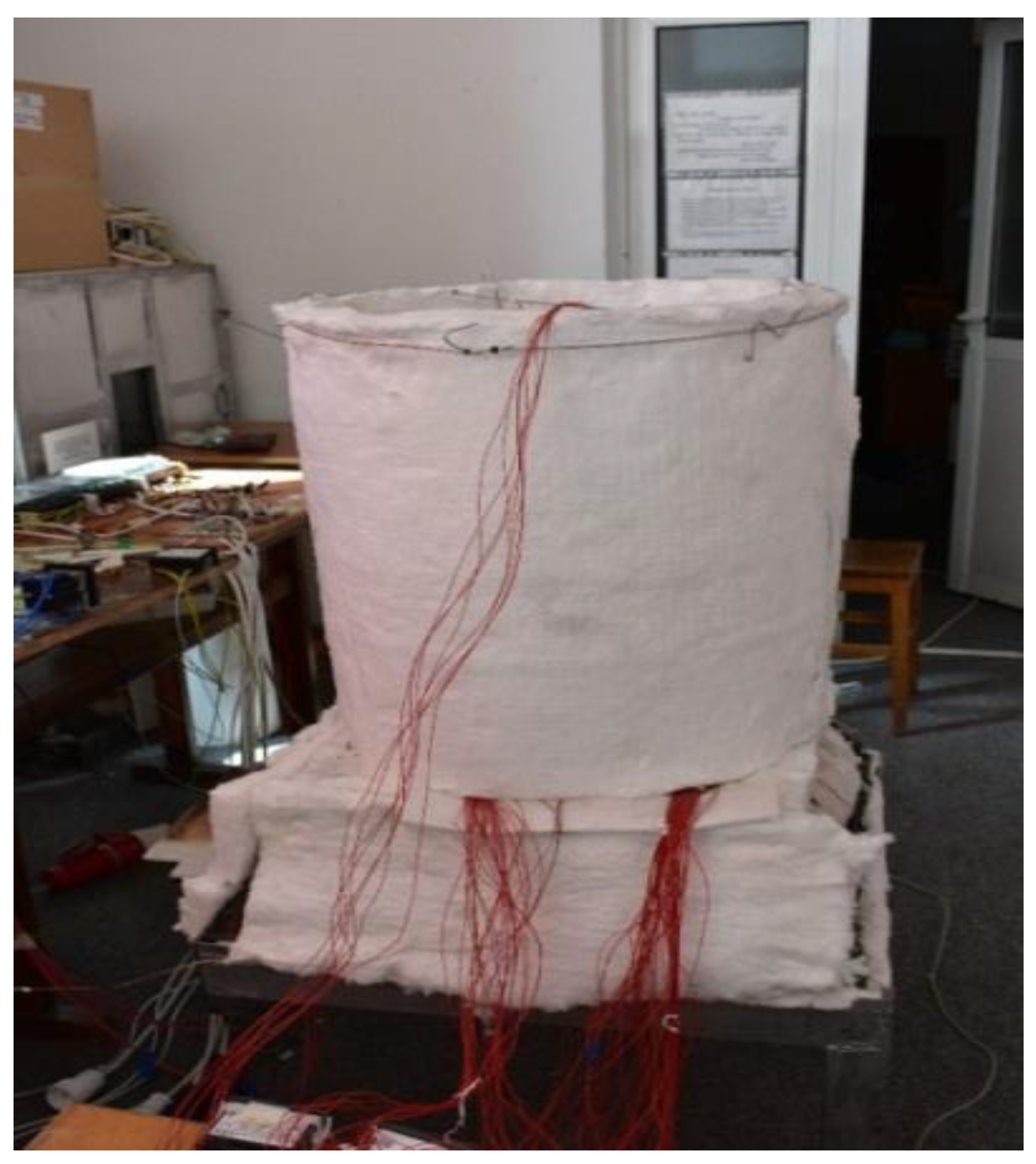
- Placing the structural element 1 on the assembled stand, by interposing between them a segment of thermal insulating mattress on the effective placement area (effective contact area), in order to ensure a perfect contact without thermal losses (Figure 6);
- Mounting, on the lower plate of the tested structural element as close as possible to their junction area, a thermocouple type K, which will be connected to the temperature controller ATR121B, in order to monitor the desired nominal temperature at the base of the structural element;
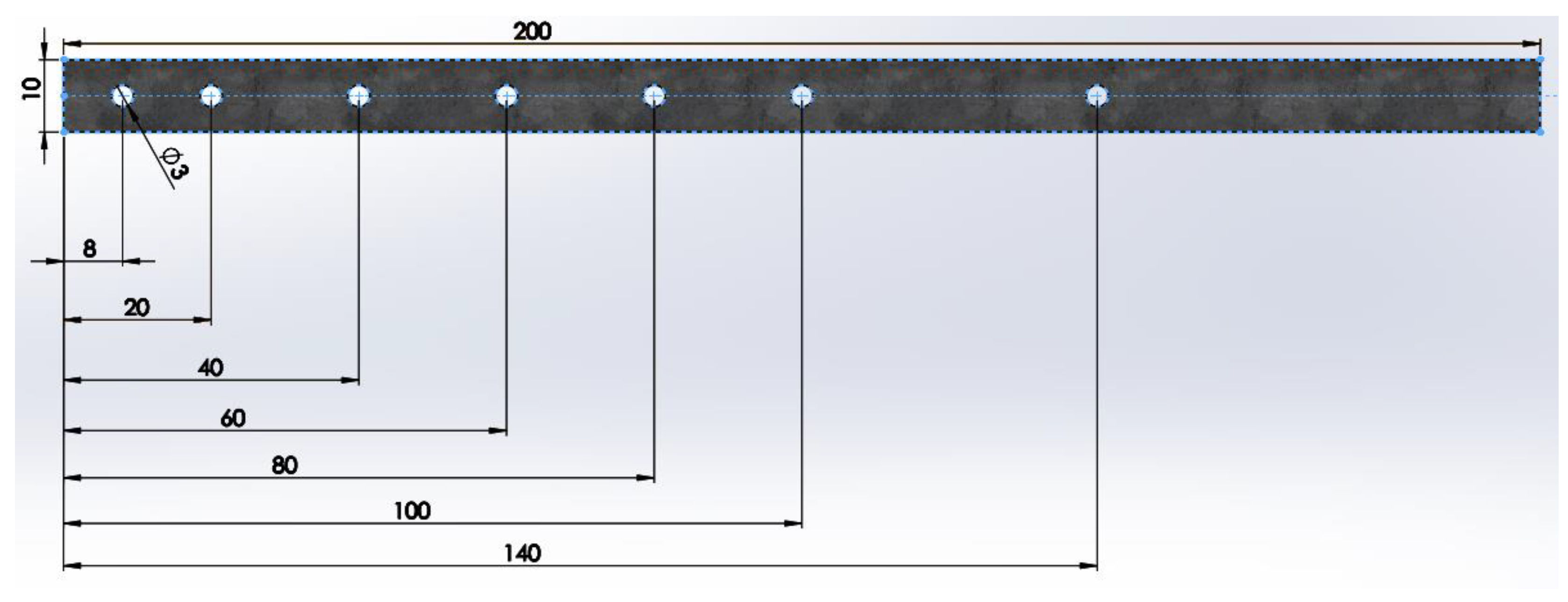
- Mounting on the tested structural element all the thermoresistors type PT 100-402 at the level of the dimensions, according to those specified above;
- Connecting these thermoresistors to the data acquisition system;
- Checking the proper operation of all thermoresistors, as well as the type K thermocouple;
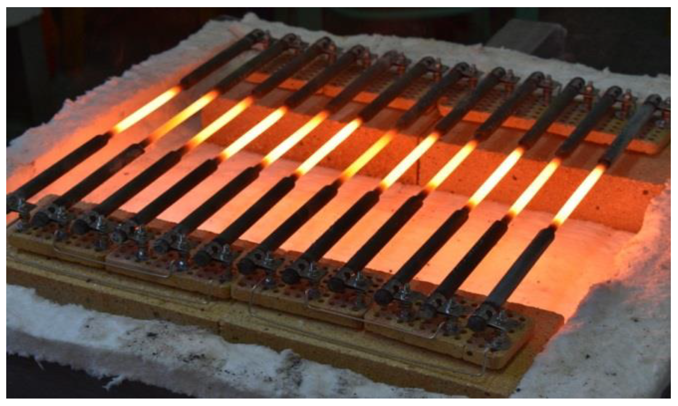
- Selection of the nominal temperature and the heating stage;
- Connecting the heating installation to the 380 V power supply;
- Starting the installation with the help of the main switch;
- Monitoring the achievement of the stabilized nominal temperature with the help of the data acquisition system,
- Additional recording, at the thermal level of the stabilized regime, of the consumed electricity , as well as of the time necessary to reach this regime;
- Repeating the previous steps in order to reach all the nominal temperatures of .
- Some observations can be made:
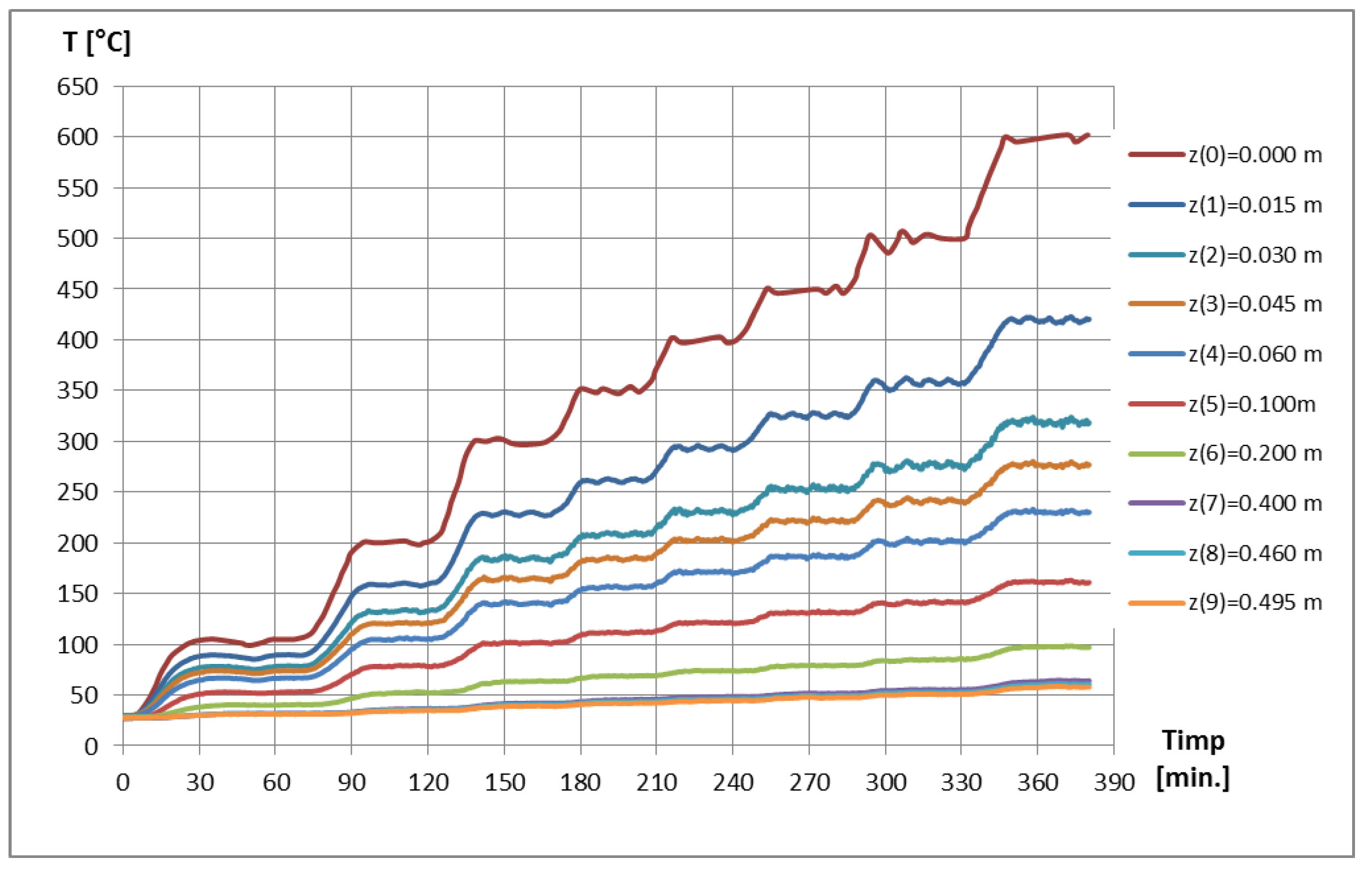
- The ATR121B temperature controller also has the self-learning function; practically, after the first cycle of reaching the nominal temperature , it will ensure the temperature regulation within very determined limits. Thus, for example, based on the measurements performed at one , the thermal oscillations related to the adjustment were of maximum ;
- A stabilized temperature regime was considered to be achieved when at the level of the last thermoresistance PT 100-402 (near the upper part of the tested structural element) and the maximum temperature oscillations were observed for a minimum period of .
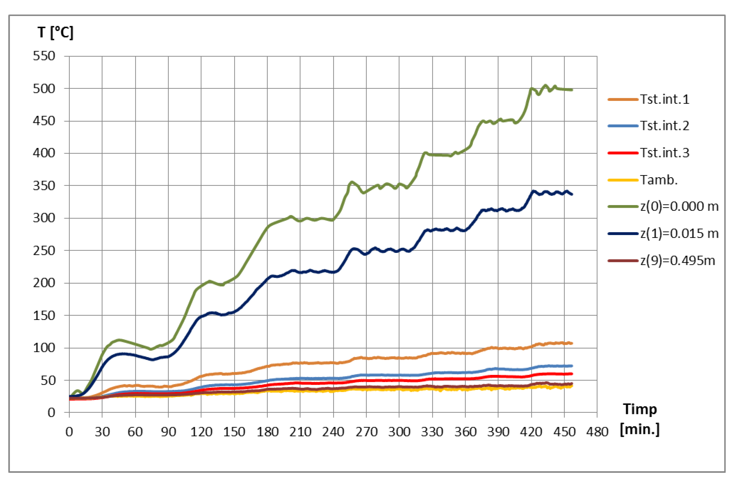
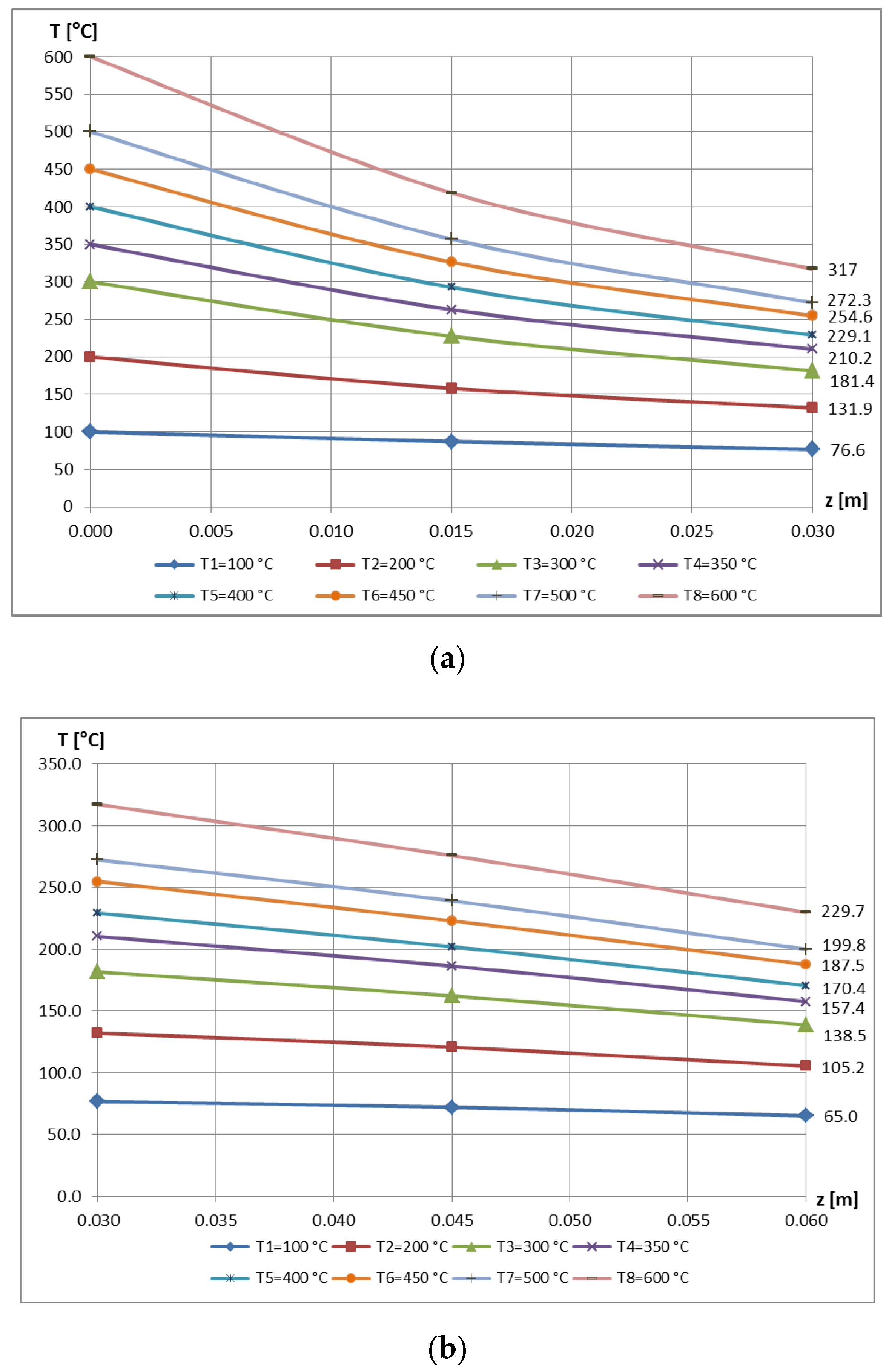
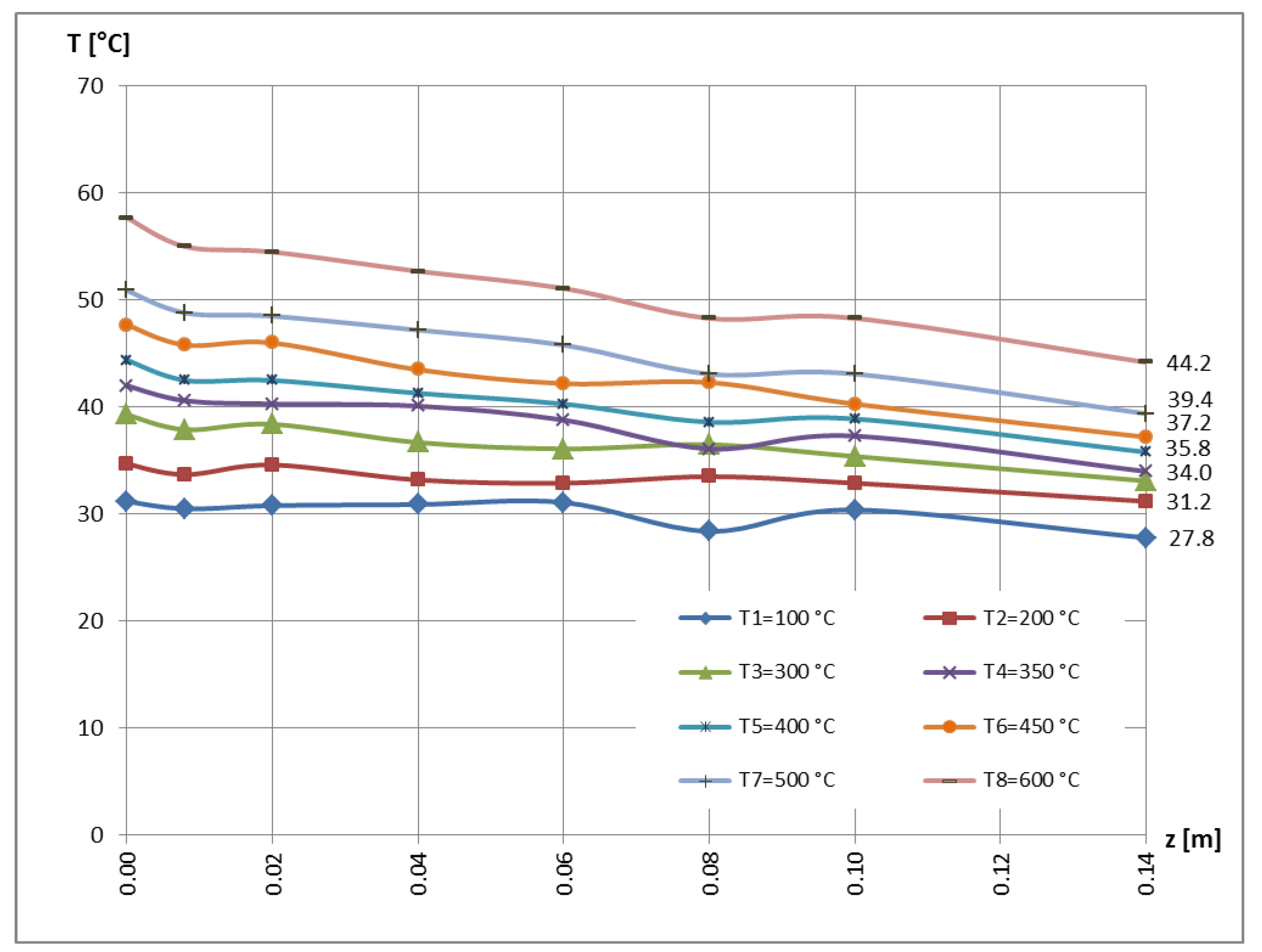
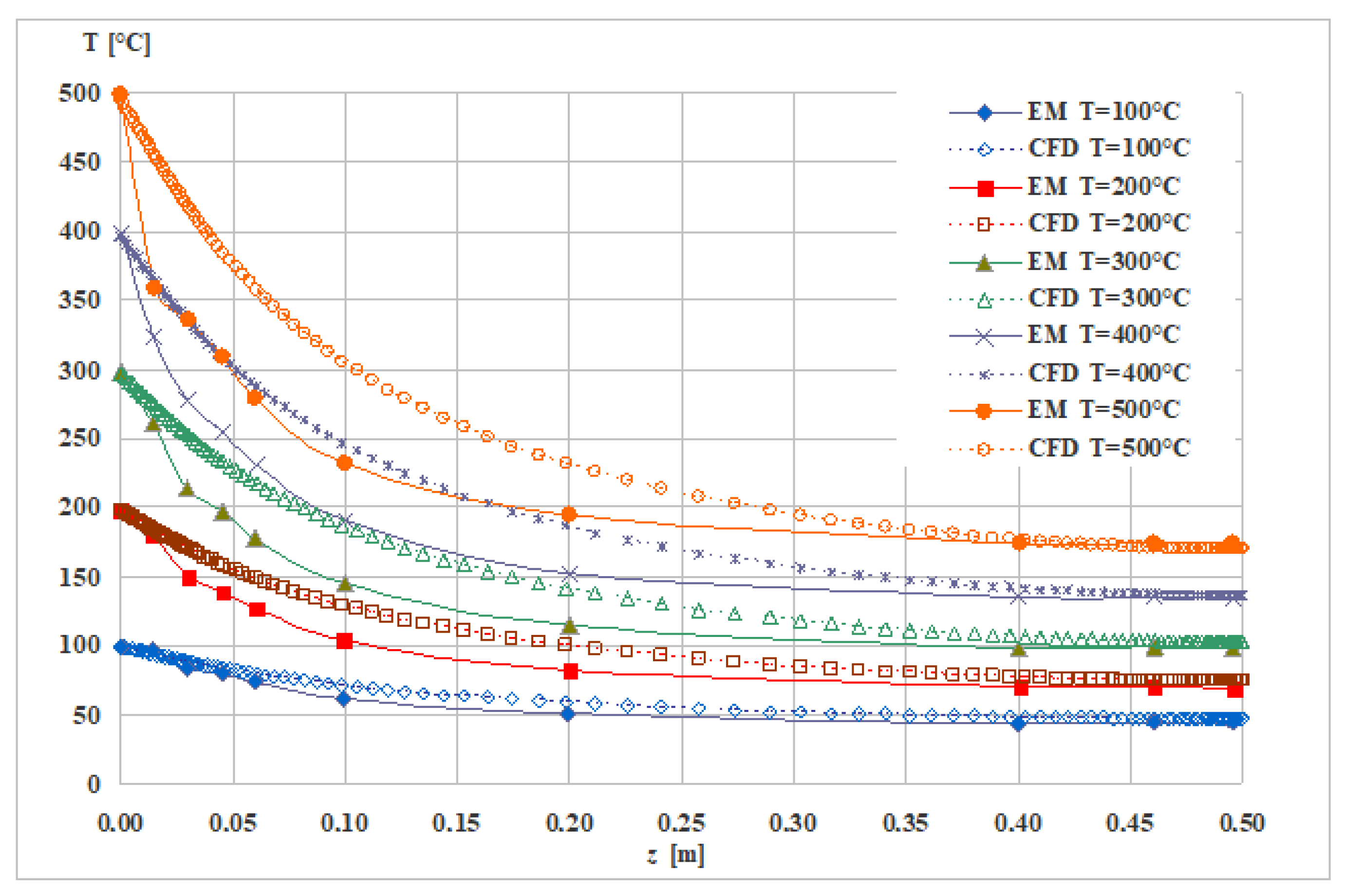
3. Experimental Results
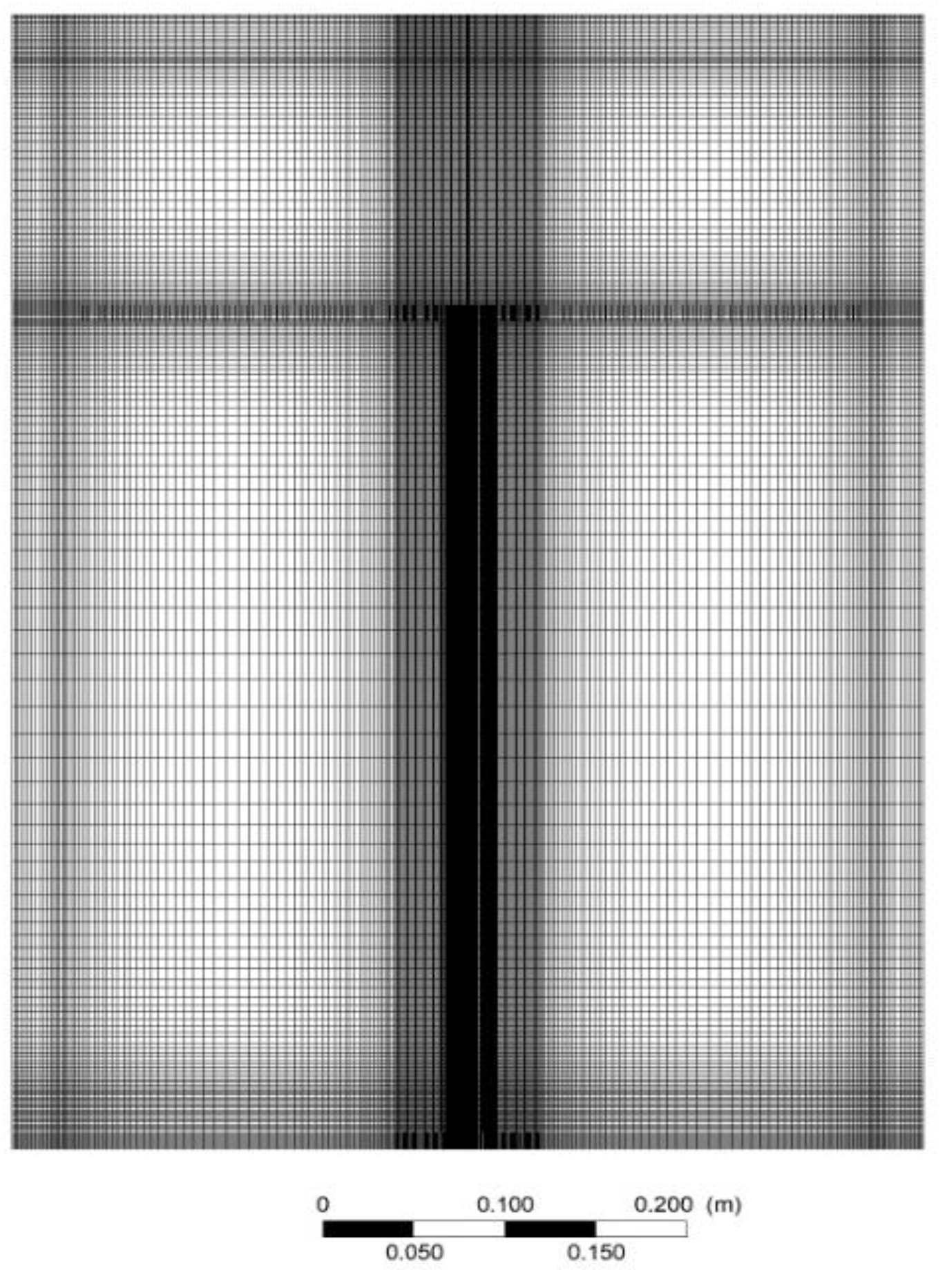
4. CFD Simulation/Numerical Solution
- Density:
- Thermal conductivity:
- The thermal radiation was neglected in the calculation;
- It was quite difficult to reproduce the exact environmental conditions from experiments during the simulation;
- The specific case of the hole beams from the condition (see Equation (5)) must be studied, where, instead of a single domain, the length of the beam has to be divided into three subdomains;
- This last demand was not realized due to the software’s particularities and consequently, in the authors’ opinion, this can be the main influence factor on the curves’ differences.
5. Conclusions
- In the paper, experimental investigations were performed on a reduced model at a scale of 1:10 of a pillar supporting an industrial hall, applying the method of reverse heating;
- A high-power electrical stand was designed, built and tested, with verified performances on a prototype (pillar segment on a natural scale), detailed in the paper [13];
- The numerical simulation of the heating phenomenon of the model was also performed, considering a thermal insulation cylinder, which delimits the space of the model from the environment;
- The obtained differences between the measured values and those from the numerical analysis may be mainly due to the fact that the software could not directly take into account the anomaly valid only on the sub-intervals of the tubular bar compared to the generally valid one (along the entire bar) from those of full sections.
- Among the goals for the near future of the authors are, among others:
- ◦
- Improvement of the numerical method, in order to be able to recognize these intervals (; ; ) from the tubular bars;
- ◦
- Validation of numerical models, ensuring obtaining results with a better precision of the measurement results;
- ◦
- Improvement of experimental and numerical investigations on bars covered with intumescent paint (so thermally protected).
Author Contributions
Funding
Institutional Review Board Statement
Informed Consent Statement
Data Availability Statement
Conflicts of Interest
Nomenclature
| a | Thermal diffusivity (m2/s); |
| A | Area (m2); |
| Bi | Biot number; |
| Constant-pressure specific heat (J/(°C kg)); | |
| Heat capacity (J/°C); | |
| F | Force (N); |
| Fo | Fourier number; |
| g | Gravitational acceleration (m/s2); |
| Gr | Grashof number; |
| l, L | Length (m); |
| Nu | Nusselt number; |
| P | Perimeter (m); |
| Pe | Péclet number; |
| Pr | Prandtl number; |
| Q | Heat (J) |
| Heat rate (W); | |
| Re | Reynolds number; |
| St | Stanton number; |
| t, T | Temperature (°C); |
| V | Volume (m3); |
| w | Velocity (m/s); |
| Scale factor corresponding to the sizes indicated in the index. | |
| Greek symbols | |
| Convection heat transfer coefficient (W/(m2 °C)); | |
| Coefficient of volume expansion (°C)−1; | |
| Thickness (m); | |
| Variation; | |
| Dynamic viscosity (kg/ms); | |
| Thermal conductivity (W/(m °C)); | |
| Kinematic viscosity (m2/s); | |
| Density (kg/m3); | |
| Shape factor (m−1); | |
| Time, shear stress (s, N/m2); | |
| Nabla operator. | |
| Subscripts | |
| x, y, z | Directions. |
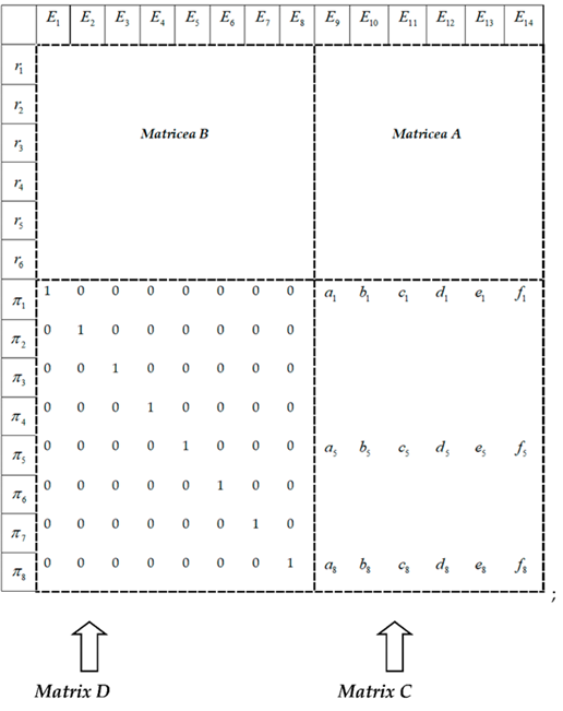
Appendix A
- ◦
- The variables, called main variables, together with their dimensions, called main dimensions, will constitute the matrix A (an invertible quadratic matrix, therefore non-singular, i.e., with ); it is clear that two or more identical dimensions should not be found among the main variables, as the condition of non-singleness would be compromised;
- ◦
- These variables in matrix A must be closely related to the experimental measurements performed on the model;
- ◦
- The main variables, through the advantages offered by MDA, must lead to obtaining a model as simple and flexible as possible, so that the experimental measurements are as safe as possible, accurate, simple and, last but not least, perfectly reproducible;
- ◦
- ◦
- The order of placement of the variables inside the matrices A and B is not restricted, remaining at the discretion of the user;
- ◦
- This Dimensional Matrix competes with the matrix , with a unit matrix of order n, and adequate , obtaining the so-called dimensional set [7,8,9,10,11], rendered in Equation (A1);
As many rows as the main
dimensions k = Nd that have
remained after defining
matrix A1. B A (A1) 2. 3. 4. … k. As many rows as the n
columns (dependent variables) of matrix B; the
number of these rows will be
identical with that of the
resulting dimensionless
quantities,1. 2. 3. 4. … … n.
References
- Schnittger, J.R. Dimensional Analysis in Design. J. Vib. Accoustic Stress Reliab. 1988, 110, 401–407. [Google Scholar]
- Carinena, J.F.; Santander, M. Dimensional Analysis. Adv. Electron. Electron Phys. 1988, 72, 181–258. [Google Scholar]
- Canagaratna, S.G. Is dimensional analysis the best we have to offer. J. Chem. Educ. 1993, 70, 40–43. [Google Scholar] [CrossRef]
- Remillard, W.J. Applying Dimensional Analysis. Am. J. Phys. 1983, 51, 137–140. [Google Scholar]
- Martins, R.D.A. The Origin of Dimensional Analysis. J. Frankl. Inst. 1981, 311, 331–337. [Google Scholar]
- Gibbings, J.C. A Logic of Dimensional Analysis. J. Phys. A Math. Gen. 1982, 15, 1991–2002. [Google Scholar]
- Trif, I.; Asztalos, Z.; Kiss, I.; Élesztos, P.; Száva, I.; Popa, G. Implementation of the Modern Dimensional Analysis in Engineering Problems-Basic Theoretical Layouts. Ann. Fac. Eng. Hunedoara 2019, 17, 73–76. [Google Scholar]
- Száva, I.; Szirtes, T.; Dani, P. An Application of Dimensional Model Theory in The Determination of the Deformation of a Structure. Eng. Mech. 2006, 13, 31–39. [Google Scholar]
- Gálfi, B.-P.; Száva, I.; Șova, D.; Vlase, S. Thermal Scaling of Transient Heat Transfer in a Round Cladded Rod with Modern Dimensional Analysis. Mathematics 2021, 9, 1875. [Google Scholar]
- Szirtes, T. The Fine Art of Modelling, SPAR. J. Eng. Technol. 1992, 1, 37. [Google Scholar]
- Szirtes, T. Applied Dimensional Analysis and Modelling; McGraw-Hill: Toronto, ON, Canada, 1998. [Google Scholar]
- Munteanu, I.R. Investigation Concerning Temperature Field Propagation along Reduced Scale Modelled Metal Structures. Ph.D. Thesis, Transilvania University of Brasov, Brasov, Romania, 2018. [Google Scholar]
- Száva, I.R.; Șova, D.; Dani, P.D.; Élesztős, P.; Száva, I.; Vlase, S. Experimental Validation of Model Heat Transfer in Rectangular Hole Beams Using Modern Dimensional Analysis. Mathematics 2022, 10, 409. [Google Scholar] [CrossRef]
- Levac, M.L.J.; Soliman, H.M.; Ormiston, S.J. Three-dimensional analysis of fluid flow and heat transfer in single- and two-layered micro-channel heat sinks. Heat Mass Transf. 2011, 47, 1375–1383. [Google Scholar]
- Alshqirate, A.A.Z.S.; Tarawneh, M.; Hammad, M. Dimensional Analysis and Empirical Correlations for Heat Transfer and Pressure Drop in Condensation and Evaporation Processes of Flow Inside Micropipes: Case Study with Carbon Dioxide (CO2). J. Braz. Soc. Mech. Sci. Eng. 2012, 34, 89–96. [Google Scholar]
- Ferro, V. Assessing flow resistance law in vegetated channels by dimensional analysis and self-similarity. Flow Meas. Instrum. 2019, 69, 101610. [Google Scholar]
- Yao, S.; Yan, K.; Lu, S.; Xu, P. Prediction and application of energy absorption characteristics of thinwalled circular tubes based on dimensional analysis. Thin Walled Struct. 2018, 130, 505–519. [Google Scholar]
- Santiago, J.G. A First Course in Dimensional Analysis; MIT Press: Cambridge, MA, USA, 2019. [Google Scholar]
- Kivade, S.B.; Murthy, C.S.N.; Vardhan, H. The use of Dimensional Analysis and Optimisation of Pneumatic Drilling Operations and Operating Parameters. J. Inst. Eng. India Ser. D 2012, 93, 31–36. [Google Scholar]
- Barlow, M.A. Dimensional Analysis & Conversion Factors; WestBow Press: Bloomington, IN, USA, 2018. [Google Scholar]
- Khan, M.A.; Shah, I.A.; Rizvi, Z.; Ahmad, J. A numerical study on the validation of hermal formulations towards the behaviours of RC beams. Mater. Today Proc. 2019, 17, 227–234. Available online: www.materialstoday.com/proceedings (accessed on 1 November 2021).
- Yen, P.H.; Wang, J.C. Power generation and electrical charge density with temperature effect of alumina nanofluids using dimensional analysis. Energy Convers. Manag. 2019, 186, 546–555. [Google Scholar]
- Dai, S.J.; Zhu, B.C.; Chen, Q. Analysis of bending strength of the rectangular hole honeycomb beam. In Applied Mechanics and Materials; Trans Tech Publications Ltd.: Freienbach, Switzerland, 2013; pp. 993–999. [Google Scholar]
- Deshwal, P.S.; Nandal, J.S. On Torsion of Rectangular Beams with Holes at the Center. Indian J. Pure Appl. Math. 1991, 22, 425–438. [Google Scholar]
- Aglan, A.A.; Redwood, R.G. Strain-Hardening Analysis of Beams with 2 WEB- Rectangular Holes. Arab. J. Sci. Eng. 1987, 12, 37–45. [Google Scholar]
- Vlase, S.; Nastac, C.; Marin, M.; Mihalcică, M. A Method for the Study of the Vibration of Mechanical Bars Systems with Symmetries. Acta Tech. Napoc. Ser. Appl. Math. Mech. Eng. 2017, 60, 539–544. [Google Scholar]
- Turzó, G.; Száva, I.R.; Gálfi, B.P.; Száva, I.; Vlase, S.; Hota, H. Temperature distribution of the straight bar, fixed into a heated plane surface. Fire Mater. 2018, 42, 202–212. [Google Scholar]
- Han, X.; Sun, X.; Li, G.; Huang, S.; Zhu, P.; Shi, C.; Zhang, T. A Repair Method for Damage in Aluminum Alloy Structures with the Cold Spray Process. Materials 2021, 14, 6957. [Google Scholar] [PubMed]
- Kim, S.; Ryu, S.; Won, J.; Kim, H.S.; Seo, T. 2-Dimensional Dynamic Analysis of Inverted Pendulum Robot With Transformable Wheel for Overcoming Steps. IEEE Robot. Autom. Lett. 2022, 7, 921–927. [Google Scholar]
- Zhang, H.; Wang, B.; Zhang, J. Parametric of dimensional analysis on iron bath gasifier. Metalurgija 2022, 61, 295–297. [Google Scholar]
- Dani, P. Theoretical and Experimental Study of the Effect of Thermal Field Propagation through Multi-Layer Protective Coatings on the State of Stresses and Strains of Metallic Structures. Ph.D. Thesis, Universitatea Transilvania din Brașov, Facultatea de inginerie Mecanică, Brașov, Romania, 2011. [Google Scholar]
- 32VDI. VDI-Wärmeatlas, 7th ed.; Verein Deutscher Ingenieure: Düsseldorf, Germany, 1994. [Google Scholar]
- Turzó, G. Temperature distribution along a straight bar sticking out from a heated plane surface and the heat flow transmitted by this bar (I)-Theoretical Approach. ANNALS Fac. Eng. Hunedoara Int. J. Eng. 2016, XIV, 49–53. [Google Scholar]
- Șova, D.; Száva, R.I.; Jármai, K.; Száva, I.; Vlase, S. Modern Method to Analyze the Heat Transfer in a Symmetric Metallic Beam with Hole. Symmetry 2022, 14, 769. [Google Scholar] [CrossRef]


Publisher’s Note: MDPI stays neutral with regard to jurisdictional claims in published maps and institutional affiliations. |
© 2022 by the authors. Licensee MDPI, Basel, Switzerland. This article is an open access article distributed under the terms and conditions of the Creative Commons Attribution (CC BY) license (https://creativecommons.org/licenses/by/4.0/).
Share and Cite
Száva, R.-I.; Bolló, B.; Bencs, P.; Jármai, K.; Száva, I.; Popa, G.; Asztalos, Z.; Vlase, S. Experimental and Numerical Studies of the Heat Transfer in Thin-Walled Rectangular Tubes under Fire. Symmetry 2022, 14, 1781. https://doi.org/10.3390/sym14091781
Száva R-I, Bolló B, Bencs P, Jármai K, Száva I, Popa G, Asztalos Z, Vlase S. Experimental and Numerical Studies of the Heat Transfer in Thin-Walled Rectangular Tubes under Fire. Symmetry. 2022; 14(9):1781. https://doi.org/10.3390/sym14091781
Chicago/Turabian StyleSzáva, Renáta-Ildikó, Betti Bolló, Péter Bencs, Károly Jármai, Ioan Száva, Gabriel Popa, Zsolt Asztalos, and Sorin Vlase. 2022. "Experimental and Numerical Studies of the Heat Transfer in Thin-Walled Rectangular Tubes under Fire" Symmetry 14, no. 9: 1781. https://doi.org/10.3390/sym14091781
APA StyleSzáva, R.-I., Bolló, B., Bencs, P., Jármai, K., Száva, I., Popa, G., Asztalos, Z., & Vlase, S. (2022). Experimental and Numerical Studies of the Heat Transfer in Thin-Walled Rectangular Tubes under Fire. Symmetry, 14(9), 1781. https://doi.org/10.3390/sym14091781