Poisson Stability in Symmetrical Impulsive Shunting Inhibitory Cellular Neural Networks with Generalized Piecewise Constant Argument

Abstract

In the paper, shunting inhibitory cellular neural networks with impulses and the generalized piecewise constant argument are under discussion. The main modeling novelty is that the impulsive part of the systems is symmetrical to the differential part. Moreover, the model depends not only on the continuous time, but also the generalized piecewise constant argument. The process is subdued to Poisson stable inputs, which cause the new type of recurrent signals. The method of included intervals, recently introduced approach of recurrent motions checking, is effectively utilized. The existence and asymptotic properties of the unique Poisson stable motion are investigated. Simulation examples for results are provided. Finally, comparing impulsive shunting inhibitory cellular neural networks with former neural network models, we discuss the significance of the components of our model.

1. Introduction

This article discusses locally connected systems, which are called cellular neural networks (CNNs). The model was introduced in 1988 by L.O. Chua and L. Yang [1,2] as a new type of information processing systems that has key characteristics of neural networks and admits important applications in parallel image and signal processing, as well as pattern recognition [3,4,5].

A class of CNNs based on shunting inhibition was introduced in paper [6] by A. Bouzerdoum and R.B. Pinter. The shunting inhibitory cellular neural networks (SICNNs) have been effectively applied in vision and image processing adaptive pattern recognition [7,8,9,10]. The layers in SICNNs are considered arrays of neurons with two dimensions. The interactions of the cells inside a single layer are subdued to the biophysical mechanism of the recurrent shunting inhibition, where the conductance is modulated by voltages of neighboring elements [6].

The impulses in neural networks are used to model the impact inputs. That is, in implementation, the state of a network can be subject to instantaneous perturbations and changes at certain moments, which may be reasoned by abrupt noise or the impact phenomenon. All this leads to a need for studies of impulsive neural networks. There are several results which explore anti-periodic, almost periodic and periodic solutions of impulse models of SICNN [11,12,13].

If one considers the impact actions as limits of continuous ones, then the jump equation of the impulsive neural network must have a functional structure identical to the differential equation. Hence, it is of great interest to consider neural networks with the structure of the impulses symmetrical to the original model. That is, the components of the impulsive equation must be analogues of components of the differential equation. Due to the similarity, the model is named the symmetrical impulsive shunting inhibitory cellular neural network (SISICNN). Previously, in the literature, non-symmetrical impulsive models were considered [11,12,13,14,15,16].

The research of recurrence types, such as periodicity, quasi periodicity and others, started within the theory of celestial dynamics and was widely spread over all areas of applied mathematics. The next position occupies the class of complex types of dynamic behavior, such as Poisson stable motions. The stability was considered by H. Poincaré as the main property in describing the complexity of celestial dynamics [17,18]. Accordingly, it is logical to suppose that Poisson stable dynamics in neural networks should be investigated based on arguments which were provided for the discussion of other types of oscillation in neuroscience. The concepts of recurrent motions and Poisson stability are conservative notions, which are focused on the theory of differential equations and dynamical systems. If H. Poincaré is the founder of the Poisson stability theory [17,18], G. Birkhoff, by introducing recurrent motions [19], established the important interrelationship of recurrent motions and the most sophisticated type of recurrence, Poisson stability.

The theoretical as well as application merits of periodicity, quasi-periodicity and almost periodicity for SICNNs have already been approved by many researchers [7,8,9,10,11,12,13]. Similarly, Poisson-stable and unpredictable motions can be considered for the same reasons. The papers [20,21,22,23,24] and book [25] can be cited as examples.

In this paper, the method of included intervals is applied to show the existence and uniqueness of discontinuous Poisson stable motions for SISICNNs. The novelties as well as contributions, present and potential, can be emphasized as follows:

• In previous studies [20,21,22,23,24,25], Poisson stability was considered for continuous systems. Here, we research the Poisson stability of discontinuous neural networks.
• Neural models, described separately by impulsive differential equations and differential equations with generalized piecewise constant arguments were considered in earlier results [11,12,13,26,27]. In this paper, we study SICNNs that include both impulses and the piecewise constant argument.
• The structure of the impulsive action is symmetrical to the differential part of the SICNN, and this is the main modeling novelty of the research. The complete symmetry can be considered not only for SICNNs, but also for Hopfield-type neural networks, Cohen–Grossberg-type neural networks, inertial neural networks and other models.
• In future investigations, the new method of included intervals can be used for neural networks with different types of discontinuity, as well as partial differential equations and functional differential equations.

The symbols $\mathbb{R}$, $\mathbb{N}$ and $\mathbb{Z}$, in the present paper, mean the sets of real numbers, natural numbers and integers, respectively.

Let us fix sequences ${\theta }_k,{\xi }_k, k\in \mathbb{Z},$ of real numbers, which satisfy ${\theta }_k<{\theta }_{k + 1}$, ${\theta }_k\le {\xi }_k\le {\theta }_{k + 1}$ for all $k\in \mathbb{Z}$, and $|{\theta }_k|\to \infty$ as $\left|k\right|\to \infty .$ It is supposed that there exist two positive real numbers $\underline{\theta }$, $\stackrel{̲}{\theta }$ such that $\underline{\theta }\le {\theta }_{k + 1} - {\theta }_k\le \stackrel{̲}{\theta }$ for all $k\in \mathbb{Z}$.

In the present study, we consider SISICNN in the form

$$\begin{array}{c}\hfill \begin{array}{c}{\displaystyle \frac{d{x}_{ij}\left(t\right)}{dt} = a_{ij}{x}_{ij}\left(t\right) - \sum _{C_{hl}\in N_r(i,j)}{C}_{ij}^{hl}f\left(x_{hl}\left(\gamma \left(t\right)\right)\right)x_{ij}\left(t\right) + v_{ij}\left(t\right),t\ne {\theta }_k,}\hfill \\ {\displaystyle \Delta x_{ij}{|}_{t = {\theta }_k} = b_{ij}{x}_{ij}\left({\theta }_k\right) + \sum _{C_{hl}\in N_r(i,j)}{D}_{ij}^{hl}g\left(x_{hl}\left({\theta }_k\right)\right)x_{ij}\left({\theta }_k\right) + h_{ijk},}\hfill \end{array}\end{array}$$

(1)

where $t\in \mathbb{R}$, $x_{ij}\in \mathbb{R}$, $b_{ij} \ne -1$ for each $i = 1,2,\dots ,m$ and $j = 1,2,\dots ,n$; $\gamma \left(t\right) = {\xi }_k,$ if ${\theta }_k\le t<{\theta }_{k + 1},k\in \mathbb{Z},$ is a piecewise constant function; $C_{ij}^{hl}\ge 0$ is the connection or coupling strength of the postsynaptic activity of the cell $C_{hl}$ transmitted to the cell $C_{ij}$; the constants $a_{ij}$ represent the passive decay rate of the cells activity; $x_{ij}$ with fixed i and j is the activity of the cell $C_{ij}$; the activation function $f\left(x_{hl}\right)$ is a positive function representing the output or firing rate of the cell $C_{hl}$; the couple $(v_{ij}\left(t\right),h_{ijk})$ is the continuous-impact external input to the cell $C_{ij}$; and $N_r(i,j)$ is the r−neighborhood of the cell $C_{ij}$, defined as

$$N_r(i,j) = \{C_{hl}:max\left\{|h - i|,|l - j|\right\}\le r,1\le h\le m,1\le l\le n\}.$$

Like the continuous components of system (1), one can say the same about the components of impacts, that is, the constant $b_{ij}$ with fixed i and j is the passive decay impulsive rate of the cell activity; the impact activation $g\left(x_{hl}\right)$ is the output localized at a moment of impact of the cell $C_{hl}$; and $D_{ij}^{hl}\ge 0$ is the strength of coupling by impacts due to the postsynaptic activity between cells $C_{hl}$ and $C_{ij}$. We assume that $f\left(s\right)$, $g\left(s\right)$ and $v\left(t\right)$ are continuous and bounded functions.

Next, we present Poisson stability for continuous and discontinuous functions and Poisson stable sequence.

Definition 1

([28]). A function $v\left(t\right):\mathbb{R}\to \mathbb{R}$, is said to be Poisson stable, provided that it is bounded, continuous and there exists a sequence $t_p$, $t_p\to \infty$ as $p\to \infty$, which satisfies $v(t + t_p)\to v\left(t\right)$ as $p\to \infty$ on each bounded interval of $\mathbb{R}$.

Definition 2

([28]). A sequence ${\kappa }_k,k\in \mathbb{Z}$, in $\mathbb{R}$ is called Poisson stable, provided that it is bounded and there exists a sequence $l_p\to \infty$, $p\in \mathbb{N}$, of positive integers, which satisfies ${\kappa }_{k + l_p}\to {\kappa }_k$ as $p\to \infty$ on bounded intervals of integers.

A piecewise continuous function $v\left(t\right):\mathbb{R}\to \mathbb{R}$, is called conditional uniform continuous, if for every number $ϵ>0$, there exists a number $\sigma >0$ which satisfies $\left|v\left(t_1\right) - v\left(t_2\right)\right|<ϵ$ whenever the points $t_1$ and $t_2$ belong to the same continuity interval and $\left|t_1 - t_2\right|<\sigma$ [26].

Let us consider the set $\mathcal{D}$ of matrix functions $\phi \left(t\right) = \left({\phi }_{ij}\left(t\right)\right)$, ${\phi }_{ij}\left(t\right):\mathbb{R}\to \mathbb{R}$, $i = 1,2,\dots ,m$, $j = 1,2,\dots ,n$, such that each entry of the function is conditional uniform continuous. The entries of functions are continuous, except a countable set of moments, where they are left-continuous. The sets of points of discontinuity are unbounded on both sides and do not have finite accumulation points. For different functions, discontinuity moments are not necessarily common.

Definition 3

([29]). Two functions $G\left(t\right) = \left\{G_{ij}\left(t\right)\right\}$ and $F\left(t\right) = \left\{F_{ij}\left(t\right)\right\}$, $i = 1,2,\dots ,m$, $j = 1,2,\dots ,n$, from $\mathcal{D}$, are called ϵ−equivalent on a bounded interval J, if the discontinuity points ${\theta }_k^G$ and ${\theta }_k^F$, $k = 1,2,\cdots ,l$, of $G\left(t\right)$ and $F\left(t\right)$ in J respectively are such that $|{\theta }_k^G - {\theta }_k^F|<ϵ$ for each $k = 1,2,\dots ,l$, and ${\displaystyle \underset{(i,j)}{max}\left|G_{ij}\left(t\right) - F_{ij}\left(t\right)\right|<ϵ}$, for each $t\in J$, $i = 1,2,\dots ,m$, $j = 1,2,\dots ,n$, except possibly those between ${\theta }_k^G$ and ${\theta }_k^F$ for all k.

In the case that G, F are ϵ−equivalent on J, we also call the functions in ϵ−neighborhoods of each other on J. The topology defined on the basis of all ϵ− neighborhoods is said to be B-topology [29].

Definition 4.

A member $\phi \left(t\right)$ of $\mathcal{D}$ is said to be a discontinuous Poisson stable function provided that there exists a sequence $t_p\to \infty$ of real numbers, which satisfies $\phi (t + t_p)\to \phi \left(t\right)$ as $p\to \infty$ in B-topology on each compact set of real numbers.

2. Methods

Extending the Poisson stable point, M. Akhmet and M.O. Fen introduced the concept of the unpredictable point [30]. Then, by assuming the separation property [30], they introduced the concept of an unpredictable function and thereby elaborated the recurrence in functional spaces. An unpredictable function is a Poisson stable function. That is, to test the unpredictability, we check the validity of the Poisson stability. In papers [20,21,22,23,24] and book [25], considering the existence and uniqueness of unpredictable solutions, we developed a new approach: the method of included intervals for asserting the Poisson stability of solutions. The method is certainly different from the method of comparability by the character of recurrence in [31,32,33,34].

A novelty in the considered model (1) is the generalized piecewise constant argument. Differential equations with generalized piecewise constant argument were introduced in 2005 by M. Akhmet [26,35,36], and they attracted the attention of scientists for their effectiveness in the fields of biology, physics, economics, and neural networks [26,27]. The proposals became the most general not only in modeling, but also very powerful in the methodological sense since the equivalent integral equations were suggested to open the research gate for methods of operators’ theory and functional analysis. The suggestions were followed by the impressive research of ordinary differential, impulsive differential, functional differential, and partial differential equations [37,38,39]. Mathematically, the generalized piecewise constant argument combines equations with retarded (delay) and advanced arguments, thereby making it possible to increase the applicability.

Impulsive systems are models for processes in which sharp interruptions of continuous processes are observed, and they are important in various fields such as medicine, mechanics, electronics, communication systems and neural networks [40,41,42]. Currently, significant results of neural networks with impulses have been obtained. Basically, in these models, the impulsive part is of a simple form. In the present work, the impulsive part completely “copies” the original model, i.e., it is identical to the SICNN. The passive decay rates $a_{ij}$, $i = 1,2,\dots ,m$, $j = 1,2,\dots ,n$, of SICNNs in [43,44] are positive. Unlike them, we do not demand the positiveness. In this paper, the coefficient can be positive, negative or zero valued, that is, due to the possibility of negative capacitance [45,46,47]. Thus, in this article, using the methods of studying impulsive systems in previous results [22,29,48], we investigate the existence of Poisson stable motion of SISCINN (1).

3. Main Results

Let us introduce the subset $\mathcal{PD}\subset \mathcal{D}$ of matrix functions $w\left(t\right) = \left(w_{ij}\left(t\right)\right)$, $i = 1,2,\dots ,m$, $j = 1,2,\dots ,n$, with the fixed set of moments of discontinuity ${\theta }_k$, $k\in \mathbb{Z}$, and Poisson stable entries which satisfy $|w_{ij}\left(t\right)|<H$, where H is a positive number, $i = 1,2,\dots ,m$, $j = 1,2,\dots ,n$. All functions of the given subset have the common convergence sequence $t_p$, $p\in \mathbb{N}$.

The function $x\left(t\right) = \left\{x_{ij}\left(t\right)\right\}$ satisfies SISICNN (1), if and only if it is a solution of the integral equation

$$\begin{array}{c}\hfill \begin{array}{c}{\displaystyle x_{ij}\left(t\right) = -{\int }_{-\infty }^t{u}_{ij}(t,s)[\sum _{C_{hl}\in N_r(i,j)}{C}_{ij}^{hl}f\left(x_{hl}\left(\gamma \left(s\right)\right)\right)x_{ij}\left(s\right) - v_{ij}(s)]ds}\hfill \\ {\displaystyle +\sum _{-\infty <{\theta }_k<t}{u}_{ij}(t,{\theta }_k+)[\sum _{C_{hl}\in N_r(i,j)}{D}_{ij}^{hl}g\left(x_{hl}\left({\theta }_k\right)\right)x_{ij}\left({\theta }_k\right) + h_{ijk}]}\hfill \end{array}\end{array}$$

for each i and j [29].

Define on $\mathcal{PD}$ the operator $\mathrm{\Phi }w\left(t\right) = \left\{{\mathrm{\Phi }}_{ij}w\left(t\right)\right\}$, $i = 1,2,\dots ,m,$ $j = 1,2,\dots ,n$, as

$$\begin{array}{ccc}& & {\displaystyle {\mathrm{\Phi }}_{ij}w\left(t\right)\equiv -{\int }_{-\infty }^t{u}_{ij}(t,s)[\sum _{C_{hl}\in N_r(i,j)}{C}_{ij}^{hl}f\left(w_{hl}\left(\gamma \left(s\right)\right)\right)w_{ij}\left(s\right) - v_{ij}(s)]ds}\hfill \\ & & {\displaystyle +\sum _{-\infty <{\theta }_k<t}{u}_{ij}(t,{\theta }_k+)[\sum _{C_{hl}\in N_r(i,j)}{D}_{ij}^{hl}g\left(w_{hl}\left({\theta }_k\right)\right)w_{ij}\left({\theta }_k\right) + h_{ijk}].}\hfill \end{array}$$

We required that system (1) satisfies the following conditions:

(C1)

The inputs $v_{ij}\left(t\right)$, $i = 1,2,\dots ,m$, $j = 1,2,\dots ,n$, are Poisson stable and the sequence $t_p$, $p\in \mathbb{N}$, is common for all inputs;

(C2)

For the sequence $\left\{h_{ijk}\right\}$, $i = 1,2,\dots , m$, $j = 1,2,\dots , n$, $k\in \mathbb{Z}$, $h_{ijk}\in \mathbb{R}$, there exists sequence $l_p$ of integers, which diverges to infinity such that $|h_{ijk + l_p} - h_{ijk}|\to 0$, as $p\to \infty$ on each bounded interval of integers and for each $i = 1,2,\dots , m$, $j = 1,2,\dots , n$;

(C3)

For the sequences $t_p, p\in \mathbb{N}$, ${\theta }_k$, and ${\xi }_k$, $k\in \mathbb{Z}$, there exists sequence $l_p$ of integers, which diverges to infinity which satisfies $|{\theta }_{k + l_p} - t_p - {\theta }_k|\to 0$ and $|{\xi }_{k + l_p} - t_p - {\xi }_k|\to 0$ as $p\to \infty$ on each finite set of integers.

Let us consider the linear homogeneous impulsive system associated with (1),

$$\begin{array}{c}\hfill \begin{array}{c}{\displaystyle \frac{d{x}_{ij}\left(t\right)}{dt} = a_{ij}{x}_{ij}\left(t\right),t\ne {\theta }_k,}\hfill \\ \Delta x_{ij}{|}_{t = {\theta }_k} = b_{ij}{x}_{ij}\left({\theta }_k\right),\hfill \end{array}\end{array}$$

(2)

where $t\in \mathbb{R}$, constants $a_{ij}, b_{ij}$, $i = 1,2,\dots , m$, $j = 1,2,\dots , n$, are real valued numbers. The transition matrix of this system has the form [29]

$$\begin{array}{ccc}\hfill & & {\displaystyle u_{ij}(t,s) = e^{a_{ij}(t - s)}{(1 + b_{ij})}^{i\left(\right[s,t\left)\right)},t\ge s,}\hfill \end{array}$$

(3)

where $i\left(\right[s,t\left)\right)$ is the number of the members of the sequence ${\theta }_k$, lying in the interval $\left[s,t\right)$.

The following conditions for the system (1) are required:

(C4)

It is true that ${\mathsf{\lambda }}_{ij} = a_{ij} + \frac{1}{\underline{\theta }}ln|1 + b_{ij}|<0$, for all $i = 1,2,\dots , m$, $j = 1,2,\dots , n$;

(C5)

$\exists M>0$, $M_{ij}>0$ such that the following equalities are valid ${\displaystyle \underset{s\in \mathbb{R}}{sup}\left|f\left(s\right)\right| + \underset{s\in \mathbb{R}}{sup}\left|g\left(s\right)\right| = M}$ and ${\displaystyle \underset{s\in \mathbb{R}}{sup}\left|v_{ij}\left(s\right)\right| + \underset{k\in \mathbb{Z}}{sup}|h_{ijk}| = M_{ij}}$;

(C6)

$\exists L>0$, which satisfies the inequality $|f\left(s_2\right) - f\left(s_1\right)| + |g\left(s_2\right) - g\left(s_1\right)|\le L|s_2 - s_1|$ for all $s_1,s_2\in \mathbb{R}$.

Due to (3) and condition $\left(C4\right)$, there exist numbers $K_{ij}\ge 1$ such that the relation

$$\begin{array}{c}\hfill \left|u_{ij}(t,s)\right|\le K_{ij}{e}^{{\mathsf{\lambda }}_{ij}(t - s)},s\le t,\end{array}$$

(4)

is valid for all $i = 1,2,\dots , m$, $j = 1,2,\dots , n$ [29].

We also need the following conditions:

$$\begin{array}{cc}\left(\mathrm{C}7\right)& \frac{K_{ij}{M}_{ij}\left(\frac{1}{-{\mathsf{\lambda }}_{ij}} + \frac{1}{1 - e^{{\mathsf{\lambda }}_{ij}\underline{\theta }}}\right)}{1 - K_{ij}M(\frac{{\sum }_{C_{hl}\in N_r(i,j)}{C}_{ij}^{hl}}{-{\mathsf{\lambda }}_{ij}} + \frac{{\sum }_{C_{hl}\in N_r(i,j)}{D}_{ij}^{hl}}{1 - e^{{\mathsf{\lambda }}_{ij}\underline{\theta }}})}<H\hfill \\ \left(\mathrm{C}8\right)& K_{ij}(M + LH)\left(\frac{{\sum }_{C_{hl}\in N_r(i,j)}{C}_{ij}^{hl}}{-{\mathsf{\lambda }}_{ij}} + \frac{{\sum }_{C_{hl}\in N_r(i,j)}{D}_{ij}^{hl}}{1 - e^{{\mathsf{\lambda }}_{ij}\underline{\theta }}}\right)<1\hfill \\ \left(\mathrm{C}9\right)& \stackrel{̲}{\theta }\left[(|a_{ij}| + M{\sum }_{C_{hl}\in N_r(i,j)}{C}_{ij}^{hl}\left)\right(1 + LH\stackrel{̲}{\theta }{\sum }_{C_{hl}\in N_r(i,j)}{C}_{ij}^{hl})e^{\left(|a_{ij}| + M{\sum }_{C_{hl}\in N_r(i,j)}{C}_{ij}^{hl}\right)\stackrel{̲}{\theta }} + LH{\sum }_{C_{hl}\in N_r(i,j)}{C}_{ij}^{hl}\right]<1.\hfill \end{array}$$

Let us accept the following notation

$$\begin{array}{c}\hfill \begin{array}{c}{N}_{ij} = {(1 - \stackrel{̲}{\theta }[(|a_{ij}| + M\sum _{C_{hl}\in N_r(i,j)}{C}_{ij}^{hl})(1 + LH\stackrel{̲}{\theta }\sum _{C_{hl}\in N_r(i,j)}{C}_{ij}^{hl})e^{\left(|a_{ij}| + {\sum }_{C_{hl}\in N_r(i,j)}{C}_{ij}^{hl}\right)\stackrel{̲}{\theta }} + LH\sum _{C_{hl}\in N_r(i,j)}{C}_{ij}^{hl}])}^{ - 1}.\hfill \end{array}\end{array}$$

(5)

(C10)

${\mathsf{\lambda }}_{ij} + \left(M + LH{N}_{ij}\right){\sum }_{C_{hl}\in N_r(i,j)}{C}_{ij}^{hl} + \frac{1}{\underline{\theta }}ln(M + LH){\sum }_{C_{hl}\in N_r(i,j)}{D}_{ij}^{hl}<0$.

Theorem 1.

The SISICNN (1) admits a unique bounded on $\mathbb{R}$ discontinuous Poisson stable motion, provided conditions $\left(C1\right)$–$\left(C8\right)$.

Proof. 

We will prove that system (1) possesses a unique discontinuous Poisson stable solution by using the contraction mapping principle.

Let us show $\mathrm{\Phi }\left(\mathcal{PD}\right)\subseteq \mathcal{PD}.$ If $w\left(t\right)$ belongs to $\mathcal{PD},$ then

$$\begin{array}{ccc}& & {\displaystyle |{\mathrm{\Phi }}_{ij}w\left(t\right)|\le {\int }_{-\infty }^t{K}_{ij}{e}^{{\mathsf{\lambda }}_{ij}(t - s)}(MH\sum _{C_{hl}\in N_r(i,j)}{C}_{ij}^{hl} + M_{ij})ds}\hfill \\ & & +\sum _{-\infty <{\theta }_k<t}{K}_{ij}{e}^{{\mathsf{\lambda }}_{ij}(t - {\theta }_k)}(MH\sum _{C_{hl}\in N_r(i,j)}{D}_{ij}^{hl} + M_{ij}).\hfill \end{array}$$

Making use of the inequality ${\displaystyle \sum _{-\infty <{\theta }_k<t}{e}^{{\mathsf{\lambda }}_{ij}(t - {\theta }_k)}\le \frac{1}{1 - e^{{\mathsf{\lambda }}_{ij}\underline{\theta }}},}$ one can obtain that

$$\begin{array}{ccc}& & {\displaystyle |{\mathrm{\Phi }}_{ij}w\left(t\right)|\le \frac{K_{ij}}{-{\mathsf{\lambda }}_{ij}}(MH\sum _{C_{hl}\in N_r(i,j)}{C}_{ij}^{hl} + M_{ij}) + \frac{K_{ij}}{1 - e^{{\mathsf{\lambda }}_{ij}\underline{\theta }}}(MH\sum _{C_{hl}\in N_r(i,j)}{D}_{ij}^{hl} + M_{ij}).}\hfill \end{array}$$

From the last inequality and condition $\left(C7\right)$, it follows that $|{\mathrm{\Phi }}_{ij}w(t)|<H.$

Fix an arbitrary number $ϵ>0$ and a compact interval $[a,b]$, where $b>a$. We will prove for sufficiently large n that the inequality $|{\mathrm{\Phi }}_{ij}w(t + t_p) - {\mathrm{\Phi }}_{ij}w(t)|<ϵ$ is satisfied for each t in $[a,b].$ Choose numbers $c<a$ and ${\zeta }_{\epsilon }>0$ such that

$$\begin{array}{c}\hfill \frac{{\mathcal{K}}_{ij}\left({\sum }_{C_{hl}\in N_r(i,j)}{C}_{ij}^{hl}MH + M_{ij}\right) + 2K_{ij}\left({\sum }_{C_{hl}\in N_r(i,j)}{C}_{ij}^{hl}(L{H}^2 + MH) + M_{ij}\right)}{-{\mathsf{\lambda }}_{ij}}{e}^{{\mathsf{\lambda }}_{ij}(a - c)}<\frac{ϵ}{7},\end{array}$$

(6)

$$\begin{array}{c}\hfill \frac{{\mathcal{K}}_{ij}\left({\sum }_{C_{hl}\in N_r(i,j)}{C}_{ij}^{hl}MH + M_{ij}\right) + 2K_{ij}\left({\sum }_{C_{hl}\in N_r(i,j)}{C}_{ij}^{hl}(L{H}^2 + MH) + M_{ij}\right)}{-{\mathsf{\lambda }}_{ij}(1 - e^{{\mathsf{\lambda }}_{ij}\underline{\theta }})}(e^{ - {\mathsf{\lambda }}_{ij}{\zeta }_{\epsilon }} - 1)<\frac{ϵ}{7},\end{array}$$

(7)

$$\begin{array}{c}\hfill \frac{K_{ij}}{1 - e^{{\mathsf{\lambda }}_{ij}\underline{\theta }}}[(\sum _{C_{hl}\in N_r(i,j)}{D}_{ij}^{hl}MH + M_{ij}) + K_{ij}(\sum _{C_{hl}\in N_r(i,j)}{D}_{ij}^{hl}(LH + M) + 1)]{\zeta }_{\epsilon }<\frac{ϵ}{7},\end{array}$$

(8)

$$\begin{array}{c}\hfill \frac{2K_{ij}}{1 - e^{{\mathsf{\lambda }}_{ij}\underline{\theta }}}(\sum _{C_{hl}\in N_r(i,j)}{D}_{ij}^{hl}(L{H}^2 + 2MH) + 2M_{ij})e^{{\mathsf{\lambda }}_{ij}(a - c)}<\frac{ϵ}{7}\end{array}$$

(9)

and

$$\begin{array}{c}\hfill \frac{K_{ij}}{-{\mathsf{\lambda }}_{ij}}\left[\sum _{C_{hl}\in N_r(i,j)}{C}_{ij}^{hl}M + 1\right]{\zeta }_{\epsilon }<\frac{ϵ}{7}.\end{array}$$

(10)

Consider the number p sufficiently large for $|w_{hl}\left({\theta }_{k + l_p}\right) - w_{hl}\left({\theta }_k\right)|<{\zeta }_{\epsilon }$, $|h_{ijk + l_p} - h_{ijk}|<{\zeta }_{\epsilon }$, $|{\theta }_{k + l_p} - t_p - {\theta }_k|<{\zeta }_{\epsilon }$, whenever ${\theta }_k\in [c,b],k\in \mathbb{Z}$ and $|w_{hl}(t + t_p) - w_{hl}\left(t\right)|<{\zeta }_{\epsilon }$, $|v_{ij}(t + t_p) - v_{ij}\left(t\right)|<{\zeta }_{\epsilon }$ for all $t\in [c,b]$, $i = 1,2,\dots ,m$, $j = 1,2,\dots ,n$.

For a fixed $t\in [a,b]$, we assume, without loss of generality, that ${\theta }_k\le {\theta }_{k + l_p} - t_p$ and ${\theta }_k\le {\theta }_{k + l_p} - t_p = c<{\theta }_{k + 1}<{\theta }_{k + 2}<\cdots <{\theta }_{k + d}\le {\theta }_{k + d + {ł}_p} - t_n\le t<{\theta }_{k + d + 1}$ so that there exist exactly d moments of discontinuity in the interval $[c,t].$ Moreover, assume that

$$\begin{array}{c}\hfill \frac{2K_{ij}LH}{ -{\mathsf{\lambda }}_{ij}}\sum _{C_{hl}\in N_r(i,j)}{C}_{ij}^{hl}(d + 1)(1 - e^{{\mathsf{\lambda }}_{ij}\stackrel{̲}{\theta }}){\zeta }_{\epsilon }<\frac{ϵ}{7},\end{array}$$

(11)

$$\begin{array}{c}\hfill \frac{2K_{ij}LH}{ -{\mathsf{\lambda }}_{ij}}\sum _{C_{hl}\in N_r(i,j)}{C}_{ij}^{hl}Hd(e^{ - {\mathsf{\lambda }}_{ij}{\zeta }_{\epsilon }} - 1)<\frac{ϵ}{7}.\end{array}$$

(12)

If $t\in [a,b]$, then we have

$$\begin{array}{ccc}& & |{\mathrm{\Phi }}_{ij}w(t + t_p) - {\mathrm{\Phi }}_{ij}w\left(t\right)|\hfill \\ & & {\displaystyle \le {\int }_{-\infty }^c|u_{ij}(t + t_p,s + t_p) - u_{ij}(t,s)|}\hfill \\ & & \times \left[\sum _{C_{hl}\in N_r(i,j)}{C}_{ij}^{hl}|f\left(w_{hl}\left(\gamma (s + t_p)\right)\right)\left|\right|w_{ij}(s + t_p)\left|\right|v_{ij}(s + t_p)|\right]ds\hfill \\ & & {\displaystyle +\sum _{-\infty <{\theta }_k<c}|u_{ij}(t + t_p,{\theta }_{k + l_p}+) - u_{ij}(t,{\theta }_k+)|}\hfill \\ & & \times \left[\sum _{C_{hl}\in N_r(i,j)}{D}_{ij}^{hl}|g\left(w_{hl}\left({\theta }_{k + l_p}\right)\right)\left|\right|w_{ij}\left({\theta }_{k + l_p}\right)| + |h_{ijk + l_p}|\right]\hfill \\ & & {\displaystyle +{\int }_c^t|u_{ij}(t + t_p,s + t_p) - u_{ij}(t,s)|}\hfill \\ & & \times \left[\sum _{C_{hl}\in N_r(i,j)}{C}_{ij}^{hl}|f\left(w_{hl}\left(\gamma (s + t_p)\right)\right)\left|\right|w_{ij}(s + t_p)| + |v_{ij}(s + t_p)|\right]ds\hfill \\ & & {\displaystyle +\sum _{c\le {\theta }_k<t}|u_{ij}(t + t_p,{\theta }_{k + l_p} + ) - u_{ij}(t,{\theta }_k + )|}\hfill \\ & & \times \left[\sum _{C_{hl}\in N_r(i,j)}{D}_{ij}^{hl}|g\left(w_{hl}\left({\theta }_{k + l_p}\right)\right)\left|\right|w_{ij}\left({\theta }_{k + l_p}\right)| + |h_{ijk + l_p}|\right]\hfill \\ & & {\displaystyle +{\int }_{-\infty }^c\left|u_{ij}(t,s)\right|[\sum _{C_{hl}\in N_r(i,j)}{C}_{ij}^{hl}|[f\left(w_{hl}\left(\gamma (s + t_p)\right)\right) - f\left(w_{hl}\left(\gamma \left(s\right)\right)\right)]w_{ij}(s + t_p)}\hfill \\ & & +f\left(w_{hl}\left(\gamma \left(s\right)\right)\right)[w_{ij}(s + t_p) - w_{ij}\left(s\right)][v_{ij}(s + t_p) - v_{ij}\left(s\right)]\left|\right]ds + \hfill \\ & & {\displaystyle +\sum _{-\infty <{\theta }_k<c}|u_{ij}(t,{\theta }_k+)|[\sum _{C_{hl}\in N_r(i,j)}{D}_{ij}^{hl}|[g\left(w_{hl}\left({\theta }_{k + l_p}\right)\right) - g\left(w_{hl}\left({\theta }_k\right)\right)]w_{ij}\left({\theta }_{k + l_p}\right)}\hfill \\ & & +g\left(w_{hl}\left({\theta }_k\right)\right)[w_{ij}\left({\theta }_{k + l_p}\right) - w_{ij}\left({\theta }_k\right)] + [h_{ijk + l_p} - h_{ijk}]\left|\right]\hfill \\ & & {\displaystyle +{\int }_c^t\left|u_{ij}(t,s)\right|\left[\sum _{C_{hl}\in N_r(i,j)}{C}_{ij}^{hl}\right|[f\left(w_{hl}\left(\gamma (s + t_p)\right)\right) - f\left(w_{hl}\left(\gamma \left(s\right)\right)\right)]w_{ij}(s + t_p)}\hfill \\ & & +f\left(w_{hl}\left(\gamma \left(s\right)\right)\right)[w_{ij}(s + t_p) - w_{ij}\left(s\right)] + [v_{ij}(s + t_p) - v_{ij}\left(s\right)]\left|\right]ds\hfill \\ & & {\displaystyle +\sum _{c\le {\theta }_k<t}\left|u_{ij}(t,{\theta }_k + )\right|\left[\sum _{C_{hl}\in N_r(i,j)}{D}_{ij}^{hl}\right|[g\left(w_{hl}\left({\theta }_{k + l_p}\right)\right) - g\left(w_{hl}\left({\theta }_k\right)\right)]w_{ij}\left({\theta }_{k + l_p}\right)}\hfill \\ & & +g\left(w_{hl}\left({\theta }_k\right)\right)[w_{ij}\left({\theta }_{k + l_p}\right) - w_{ij}\left({\theta }_k\right)] + [h_{ijk + l_p} - h_{ijk}]\left|\right].\hfill \end{array}$$

By virtue of Appendix A Lemma A1, one can obtain

$$\begin{array}{ccc}& & {\displaystyle {\int }_{-\infty }^c|u_{ij}(t + t_p,s + t_n) - u_{ij}(t,s)|}\hfill \\ & & \times \left[\sum _{C_{hl}\in N_r(i,j)}{C}_{ij}^{hl}|f\left(w_{hl}\left(\gamma (s + t_p)\right)\right)\left|\right|w_{ij}(s + t_p)| + |v_{ij}(s + t_p)|\right]ds\hfill \\ & & {\displaystyle +\sum _{-\infty <{\theta }_k<c}|u_{ij}(t + t_p,{\theta }_{k + l_p} + ) - u_{ij}(t,{\theta }_k + )|}\hfill \\ & & \times \left[\sum _{C_{hl}\in N_r(i,j)}{D}_{ij}^{hl}|g\left(w_{hl}\left({\theta }_{k + l_p}\right)\right)\left|\right|w_{ij}\left({\theta }_{k + l_p}\right)| + |h_{ijk + l_p}|\right]\hfill \\ & & \le \underset{-\infty }{\overset{c}{\int }}\mathcal{K}{e}^{{\mathsf{\lambda }}_{ij}(t - s)}[\sum _{C_{hl}\in N_r(i,j)}{C}_{ij}^{hl}MH + M_{ij}]ds\hfill \\ & & {\displaystyle +\sum _{i^{\prime } = -\infty }^{k - 1}[K{e}^{{\mathsf{\lambda }}_{ij}(t + t_p - {\theta }_{i^{\prime } + 1 + l_p})} + K{e}^{{\mathsf{\lambda }}_{ij}(t - {\theta }_{i^{\prime } + 1})}][\sum _{C_{hl}\in N_r(i,j)}{D}_{ij}^{hl}MH + M_{ij}]}\hfill \\ & & <[\sum _{C_{hl}\in N_r(i,j)}{C}_{ij}^{hl}MH + M_{ij}]\frac{\mathcal{K}}{|{\mathsf{\lambda }}_{ij}|}{e}^{{\mathsf{\lambda }}_{ij}(t - s)} + [\sum _{C_{hl}\in N_r(i,j)}{D}_{ij}^{hl}MH + M_{ij}]\frac{2K}{1 - e^{{\mathsf{\lambda }}_{ij}\underline{\theta }}}{e}^{{\mathsf{\lambda }}_{ij}(t - {\theta }_{i^{\prime } + 1})}\hfill \\ & & \le [\sum _{C_{hl}\in N_r(i,j)}{C}_{ij}^{hl}MH + M_{ij}]\frac{\mathcal{K}}{|{\mathsf{\lambda }}_{ij}|}{e}^{{\mathsf{\lambda }}_{ij}(a - c)} + [\sum _{C_{hl}\in N_r(i,j)}{D}_{ij}^{hl}MH + M_{ij}]\frac{2K}{1 - e^{{\mathsf{\lambda }}_{ij}\underline{\theta }}}{e}^{{\mathsf{\lambda }}_{ij}(a - c)}\hfill \end{array}$$

if $i = 1,2,\dots ,m$, $j = 1,2,\dots ,n$. Additionally, we obtain

$$\begin{array}{ccc}& & \underset{c}{\overset{t}{\int }}|u_{ij}(t + t_p,s + t_n) - u_{ij}(t,s)|\hfill \\ & & \times \left[\sum _{C_{hl}\in N_r(i,j)}{C}_{ij}^{hl}|f\left(w_{hl}\left(\gamma (s + t_p)\right)\right)\left|\right|w_{ij}(s + t_p)| + |v_{ij}(s + t_p)|\right]ds\hfill \\ & & {\displaystyle +\sum _{c\le {\theta }_k<t}|u_{ij}(t + t_p,{\theta }_{k + l_p} + ) - u_{ij}(t,{\theta }_k + )|}\hfill \\ & & \times \left[\sum _{C_{hl}\in N_r(i,j)}{D}_{ij}^{hl}|g\left(w_{hl}\left({\theta }_{k + l_p}\right)\right)\left|\right|w_{ij}\left({\theta }_{k + l_p}\right)| + |h_{ijk + l_p}|\right]\hfill \\ & & {\displaystyle \le \sum _{i^{\prime } = k}^{k + d - 1}\underset{{\theta }_{i^{\prime } + 1}}{\overset{{\theta }_{i^{\prime } + 1 + l_p} - t_p}{\int }}{\mathcal{K}}_{ij}{e}^{{\mathsf{\lambda }}_{ij}(t - s)}[\sum _{C_{hl}\in N_r(i,j)}{C}_{ij}^{hl}MH + M_{ij}]ds}\hfill \\ & & {\displaystyle +\sum _{i^{\prime } = k}^{k + d - 1}{K}_{ij}{e}^{{\mathsf{\lambda }}_{ij}(t - {\theta }_{i^{\prime } + 1})}{\zeta }_{\epsilon }[\sum _{C_{hl}\in N_r(i,j)}{D}_{ij}^{hl}MH + M_{ij}]}\hfill \\ & & <[\sum _{C_{hl}\in N_r(i,j)}C{ij}^{hl}MH + M_{ij}]\frac{{\mathcal{K}}_{ij}(e^{-{\mathsf{\lambda }}_{ij}{\zeta }_{\epsilon }} - 1)}{-{\mathsf{\lambda }}_{ij}(1 - e^{{\mathsf{\lambda }}_{ij}\underline{\theta }})}\hfill \\ & & +[\sum _{C_{hl}\in N_r(i,j)}{D}_{ij}^{hl}MH + M_{ij}]\frac{K_{ij}{\zeta }_{\epsilon }}{1 - e^{{\mathsf{\lambda }}_{ij}\underline{\theta }}}\hfill \end{array}$$

for all $i = 1,2,\dots ,m$, $j = 1,2,\dots ,n$.

Similarly, one can see that

$$\begin{array}{ccc}& & {\displaystyle {\int }_{-\infty }^c|u_{ij}(t,s)\left|\right[\sum _{C_{hl}\in N_r(i,j)}{C}_{ij}^{hl}\left[\right|f\left(w_{hl}\left(\gamma (s + t_p)\right)\right) - f\left(w_{hl}\left(\gamma \left(s\right)\right)\right)\left|\right|w_{ij}(s + t_p)|}\hfill \\ & & +|f\left(w_{hl}\left(\gamma \left(s\right)\right)\right)\left|\right|w_{ij}(s + t_p) - w_{ij}\left(s\right)\left|\right] + |v_{ij}(s + t_p) - v_{ij}\left(s\right)\left|\right]ds\hfill \\ & & {\displaystyle +\sum _{-\infty <{\theta }_k<c}|u_{ij}(t,{\theta }_k + )\left|\right[\sum _{C_{hl}\in N_r(i,j)}{D}_{ij}^{hl}\left[\right|g\left(w_{hl}\left({\theta }_{k + l_p}\right)\right) - g\left(w_{hl}\left({\theta }_k\right)\right)\left|\right|w_{ij}\left({\theta }_{k + l_p}\right)|}\hfill \\ & & +|g\left(w_{hl}\left({\theta }_k\right)\right)\left|\right|w_{ij}\left({\theta }_{k + l_p}\right) - w_{ij}\left({\theta }_k\right)\left|\right] + |h_{ijk + l_p} - h_{ijk}\left|\right]\hfill \\ & & \le \underset{-\infty }{\overset{c}{\int }}{K}_{ij}{e}^{{\mathsf{\lambda }}_{ij}(t - s)}\left[\sum _{C_{hl}\in N_r(i,j)}{C}_{ij}^{hl}(2L{H}^2 + 2MH) + 2M_{ij}\right]ds\hfill \\ & & {\displaystyle +\sum _{i^{\prime } = -\infty }^{k - 1}{K}_{ij}{e}^{{\mathsf{\lambda }}_{ij}(t - {\theta }_{i^{\prime } + 1})}\left[\sum _{C_{hl}\in N_r(i,j)}{D}_{ij}^{hl}(2L{H}^2 + 2MH) + 2M_{ij}\right]}\hfill \\ & & \le \frac{2K_{ij}\left[{\sum }_{C_{hl}\in N_r(i,j)}{C}_{ij}^{hl}(L{H}^2 + MH) + M_{ij}\right]}{-{\mathsf{\lambda }}_{ij}}{e}^{{\mathsf{\lambda }}_{ij}(a - c)}\hfill \\ & & +\frac{2K_{ij}\left[{\sum }_{C_{hl}\in N_r(i,j)}{D}_{ij}^{hl}(L{H}^2 + MH) + M_{ij}\right]}{1 - e^{ - {\mathsf{\lambda }}_{ij}\underline{\theta }}}{e}^{{\mathsf{\lambda }}_{ij}(a - c)}\hfill \end{array}$$

if $i = 1,2,\dots ,m$, $j = 1,2,\dots ,n$.

Further, we need to obtain an upper bound for the following integral

$$\begin{array}{c}\hfill {\displaystyle I\left(t\right) = \sum _{C_{hl}\in N_r(i,j)}{C}_{ij}^{hl}\underset{c}{\overset{t}{\int }}{e}^{{\mathsf{\lambda }}_{ij}(t - s)}|w_{hl}\left(\gamma (s + t_p)\right) - w_{hl}\left(\gamma \left(s\right)\right)|ds.}\end{array}$$

We evaluate $I\left(t\right)$ by considering it on finite number of sub-intervals as described below:

$$\begin{array}{c}{\displaystyle I\left(t\right) = \sum _{C_{hl}\in N_r(i,j)}{C}_{ij}^{hl}\underset{c}{\overset{{\theta }_{k + 1}}{\int }}{e}^{{\mathsf{\lambda }}_{ij}(t - s)}|w_{hl}\left(\gamma (s + t_p)\right) - w_{hl}\left(\gamma \left(s\right)\right)|ds}\hfill \\ {\displaystyle +\sum _{C_{hl}\in N_r(i,j)}{C}_{ij}^{hl}\underset{{\theta }_{k + 1}}{\overset{{\theta }_{k + 1 + l_p} - t_p}{\int }}{e}^{{\mathsf{\lambda }}_{ij}(t - s)}|w_{hl}\left(\gamma (s + t_p)\right) - w_{hl}\left(\gamma \left(s\right)\right)|ds}\hfill \\ {\displaystyle +\sum _{C_{hl}\in N_r(i,j)}{C}_{ij}^{hl}\underset{{\theta }_{k + 1 + l_p} - t_p}{\overset{{\theta }_{k + 2}}{\int }}{e}^{{\mathsf{\lambda }}_{ij}(t - s)}|w_{hl}\left(\gamma (s + t_p)\right) - w_{hl}\left(\gamma \left(s\right)\right)|ds}\hfill \\ {\displaystyle +\sum _{C_{hl}\in N_r(i,j)}{C}_{ij}^{hl}\underset{{\theta }_{k + 2}}{\overset{{\theta }_{k + 2 + l_p} - t_p}{\int }}{e}^{{\mathsf{\lambda }}_{ij}(t - s)}|w_{hl}\left(\gamma (s + t_p)\right) - w_{hl}\left(\gamma \left(s\right)\right)|ds}\hfill \\ {\displaystyle +\sum _{C_{hl}\in N_r(i,j)}{C}_{ij}^{hl}\underset{{\theta }_{k + 2 + l_p} - t_p}{\overset{{\theta }_{k + 3}}{\int }}{e}^{{\mathsf{\lambda }}_{ij}(t - s)}|w_{hl}\left(\gamma (s + t_p)\right) - w_{hl}\left(\gamma \left(s\right)\right)|ds}\hfill \\ ⋮\hfill \\ {\displaystyle +\sum _{C_{hl}\in N_r(i,j)}{C}_{ij}^{hl}\underset{{\theta }_{k + d + l_p} - t_n}{\overset{t}{\int }}{e}^{{\mathsf{\lambda }}_{ij}(t - s)}|w_{hl}\left(\gamma (s + t_n)\right) - w_{hl}\left(\gamma \left(s\right)\right)|ds}\hfill \\ {\displaystyle =\sum _{i^{\prime } = k}^{k + d - 1}{A}_{i^{\prime }} + \sum _{i^{\prime } = k}^{k + d - 1}{B}_{i^{\prime }} + \sum _{C_{hl}\in N_r(i,j)}{C}_{ij}^{hl}\underset{{\theta }_{k + d + l_p} - t_p}{\overset{t}{\int }}{e}^{{\mathsf{\lambda }}_{ij}(t - s)}|w_{hl}\left(\gamma (s + t_p)\right) - w_{hl}\left(\gamma \left(s\right)\right)|ds,}\hfill \end{array}$$

where

$${\displaystyle A_{i^{\prime }} = \sum _{C_{hl}\in N_r(i,j)}{C}_{ij}^{hl}\underset{{\theta }_{i^{\prime } + l_p} - t_p}{\overset{{\theta }_{i^{\prime } + 1}}{\int }}{e}^{{\mathsf{\lambda }}_{ij}(t - s)}|w_{hl}\left(\gamma (s + t_p)\right) - w_{hl}\left(\gamma \left(s\right)\right)|ds}$$

and

$${\displaystyle B_{i^{\prime }} = \sum _{C_{hl}\in N_r(i,j)}{C}_{ij}^{hl}\underset{{\theta }_{i^{\prime } + 1}}{\overset{{\theta }_{i^{\prime } + 1 + l_p} - t_p}{\int }}{e}^{{\mathsf{\lambda }}_{ij}(t - s)}|w_{hl}\left(\gamma (s + t_p)\right) - w_{hl}\left(\gamma \left(s\right)\right)|ds}$$

for $i^{\prime } = k,k + 1,\dots ,k + d - 1.$ For $t\in [{\theta }_{i^{\prime } + l_p} - t_p,{\theta }_{i^{\prime } + 1}),$ $i^{\prime }\in \mathbb{Z},$ it is clear that $\gamma \left(t\right) = {\xi }_{i^{\prime }}$ and it follows from the condition $\left(C3\right)$ that $\gamma (t + t_p) = {\xi }_{i^{\prime } + l_p}.$ Using this result, we reach the following estimation:

$$\begin{array}{ccc}& & {\displaystyle A_{i^{\prime }} = \sum _{C_{hl}\in N_r(i,j)}{C}_{ij}^{hl}\underset{{\theta }_{i^{\prime } + l_p} - t_p}{\overset{{\theta }_{i^{\prime } + 1}}{\int }}{e}^{{\mathsf{\lambda }}_{ij}(t - s)}|w_{hl}\left({\xi }_{i^{\prime } + l_p}\right) - w_{hl}\left({\xi }_{i^{\prime }}\right)|ds}\hfill \\ & & {\displaystyle =\sum _{C_{hl}\in N_r(i,j)}{C}_{ij}^{hl}\underset{{\theta }_{i^{\prime } + l_p} - t_p}{\overset{{\theta }_{i^{\prime } + 1}}{\int }}{e}^{{\mathsf{\lambda }}_{ij}(t - s)}|w_{hl}({\xi }_{i^{\prime }} + t_p + o\left(1\right)) - w_{hl}\left({\xi }_{i^{\prime }}\right)|ds}\hfill \\ & & {\displaystyle \le \sum _{C_{hl}\in N_r(i,j)}{C}_{ij}^{hl}\underset{{\theta }_{i^{\prime } + l_p} - t_p}{\overset{{\theta }_{i^{\prime } + 1}}{\int }}{e}^{{\mathsf{\lambda }}_{ij}(t - s)}|w_{hl}({\xi }_{i^{\prime }} + t_p) - w_{hl}\left({\xi }_{i^{\prime }}\right)|ds}\hfill \\ & & {\displaystyle +\sum _{C_{hl}\in N_r(i,j)}{C}_{ij}^{hl}\underset{{\theta }_{i^{\prime } + l_p} - t_p}{\overset{{\theta }_{i^{\prime } + 1}}{\int }}{e}^{{\mathsf{\lambda }}_{ij}(t - s)}|w_{hl}({\xi }_{i^{\prime }} + t_p + o\left(1\right)) - w_{hl}({\xi }_{i^{\prime }} + t_p)|ds}\hfill \\ & & {\displaystyle \le \sum _{C_{hl}\in N_r(i,j)}{C}_{ij}^{hl}\underset{{\theta }_{i^{\prime } + l_p} - t_p}{\overset{{\theta }_{i^{\prime } + 1}}{\int }}{e}^{{\mathsf{\lambda }}_{ij}(t - s)}\left[{\zeta }_{\epsilon } + |w_{hl}({\xi }_{i^{\prime }} + t_p + o\left(1\right)) - w_{hl}({\xi }_{i^{\prime }} + t_p)|\right]ds.}\hfill \end{array}$$

We already know that w is a uniformly continuous function. Thus, for ${\zeta }_{\epsilon }>0$ and sufficiently large p one can find a $\rho >0$ such that $|w_{hl}({\xi }_{i^{\prime }} + t_p + o\left(1\right)) - w_{hl}({\xi }_{i^{\prime }} + t_p)|<{\zeta }_{\epsilon }$ if $|{\xi }_{i^{\prime } + l_p} - {\xi }_{i^{\prime }} - t_p|<\rho .$ This implies in turn that

$$\begin{array}{c}\hfill {\displaystyle A_{i^{\prime }}\le 2{\zeta }_{\epsilon }\sum _{C_{hl}\in N_r(i,j)}{C}_{ij}^{hl}\underset{{\theta }_{i^{\prime } - 1 + l_p} - t_p}{\overset{{\theta }_{i^{\prime }}}{\int }}{e}^{{\mathsf{\lambda }}_{ij}(t - s)}ds\le \frac{2{\zeta }_{\epsilon }}{-{\mathsf{\lambda }}_{ij}}\sum _{C_{hl}\in N_r(i,j)}{C}_{ij}^{hl}(1 - e^{{\mathsf{\lambda }}_{ij}\stackrel{̲}{\theta }}).}\end{array}$$

On the other hand, condition $\left(C3\right)$ gives us that

$$\begin{array}{c}\hfill {\displaystyle B_{i^{\prime }}\le 2H\sum _{C_{hl}\in N_r(i,j)}{C}_{ij}^{hl}\underset{{\theta }_{i^{\prime }}}{\overset{{\theta }_{i^{\prime } + l_p} - t_p}{\int }}{e}^{{\mathsf{\lambda }}_{ij}(t - s)}ds\le \frac{2H}{-{\mathsf{\lambda }}_{ij}}\sum _{C_{hl}\in N_r(i,j)}{C}_{ij}^{hl}(e^{ - {\mathsf{\lambda }}_{ij}{\zeta }_{\epsilon }} - 1).}\end{array}$$

If we use a similar approach used for the estimation of the integral $A_{i^{\prime }},$ then it follows that

$${\displaystyle \sum _{C_{hl}\in N_r(i,j)}{C}_{ij}^{hl}\underset{{\theta }_{k + d - 1 + l_p} - t_p}{\overset{t}{\int }}{e}^{{\mathsf{\lambda }}_{ij}(t - s)}|w_{hl}\left(\gamma (s + t_p)\right) - w_{hl}\left(\gamma \left(s\right)\right)|\le \frac{2{\zeta }_{\epsilon }}{ - {\mathsf{\lambda }}_{ij}}\sum _{C_{hl}\in N_r(i,j)}{C}_{ij}^{hl}(1 - e^{{\mathsf{\lambda }}_{ij}\stackrel{̲}{\theta }}).}$$

Therefore, it can be seen that

$$\begin{array}{c}\hfill I\left(t\right)\le 2{\zeta }_{\epsilon }(d + 1)\frac{{\sum }_{C_{hl}\in N_r(i,j)}{C}_{ij}^{hl}}{ - {\mathsf{\lambda }}_{ij}}(1 - e^{{\mathsf{\lambda }}_{ij}\stackrel{̲}{\theta }}) + 2Hd\frac{{\sum }_{C_{hl}\in N_r(i,j)}{C}_{ij}^{hl}}{ - {\mathsf{\lambda }}_{ij}}(e^{ - {\mathsf{\lambda }}_{ij}{\zeta }_{\epsilon }} - 1).\end{array}$$

Using the last inequality, we have

$$\begin{array}{ccc}& & {\displaystyle {\int }_c^t\left|u_{ij}(t,s)\right|[\sum _{C_{hl}\in N_r(i,j)}{C}_{ij}^{hl}|[f\left(w_{hl}\left(\gamma (s + t_p)\right)\right) - f\left(w_{hl}\left(\gamma \left(s\right)\right)\right)]w_{ij}(s + t_p)}\hfill \\ & & +f\left(w_{hl}\left(\gamma \left(s\right)\right)\right)[w_{ij}(s + t_p) - w_{ij}\left(s\right)] + [v_{ij}(s + t_p) - v_{ij}\left(s\right)]\left|\right]ds\hfill \\ & & {\displaystyle +\sum _{c\le {\theta }_k<t}\left|u_{ij}(t,{\theta }_k + )\right|[\sum _{C_{hl}\in N_r(i,j)}{D}_{ij}^{hl}|[g\left(w_{hl}\left({\theta }_{k + l_p}\right)\right) - g\left(w_{hl}\left({\theta }_k\right)\right)]w_{ij}\left({\theta }_{k + l_p}\right)}\hfill \\ & & +g\left(w_{hl}\left({\theta }_k\right)\right)[w_{ij}\left({\theta }_{k + l_p}\right) - w_{ij}\left({\theta }_k\right)] + [h_{ijk + l_p} - h_{ijk}]\left|\right]\hfill \\ & & \le \underset{c}{\overset{t}{\int }}{K}_{ij}{e}^{{\mathsf{\lambda }}_{ij}(t - s)}\left[\sum _{C_{hl}\in N_r(i,j)}{C}_{ij}^{hl}\left(LH\right|w_{hl}\left(\gamma (s + t_p)\right) - w_{hl}\left(\gamma \left(s\right)\right)| + M{\zeta }_{\epsilon }) + {\zeta }_{\epsilon }\right]ds\hfill \\ & & {\displaystyle +\sum _{i^{\prime } = k}^{k + d - 1}\underset{{\theta }_{i^{\prime } + 1}}{\overset{{\theta }_{i^{\prime } + 1 + l_p}}{\int }}{K}_{ij}{e}^{{\mathsf{\lambda }}_{ij}(t - s)}\left[\sum _{C_{hl}\in N_r(i,j)}{C}_{ij}^{hl}(2L{H}^2 + 2MH) + 2M_{ij}\right]ds}\hfill \\ & & {\displaystyle +\sum _{i^{\prime } = k}^{k + d - 1}{K}_{ij}{e}^{{\mathsf{\lambda }}_{ij}(t - {\theta }_{i^{\prime } + 1})}\left[\sum _{C_{hl}\in N_r(i,j)}{D}_{ij}^{hl}(LH{\zeta }_{\epsilon } + M{\zeta }_{\epsilon }) + {\zeta }_{\epsilon }\right]}\hfill \\ & & \le K_{ij}LH\sum _{C_{hl}\in N_r(i,j)}{C}_{ij}^{hl}\underset{c}{\overset{t}{\int }}{e}^{{\mathsf{\lambda }}_{ij}(t - s)}|w_{hl}\left(\gamma (s + t_p)\right) - w_{hl}\left(\gamma \left(s\right)\right)|ds\hfill \\ & & +K_{ij}{\zeta }_{\epsilon }\left[\sum _{C_{hl}\in N_r(i,j)}{C}_{ij}^{hl}M + 1\right]\underset{c}{\overset{t}{\int }}{e}^{{\mathsf{\lambda }}_{ij}(t - s)}ds\hfill \\ & & {\displaystyle + K_{ij}\left[\sum _{C_{hl}\in N_r(i,j)}{C}_{ij}^{hl}(2L{H}^2 + 2MH) + 2M_{ij}\right]\sum _{i^{\prime } = k}^{k + d - 1}\underset{{\theta }_{i^{\prime } + 1}}{\overset{{\theta }_{i^{\prime } + 1 + l_p}}{\int }}{e}^{{\mathsf{\lambda }}_{ij}(t - s)}ds}\hfill \\ & & {\displaystyle +K_{ij}{\zeta }_{\epsilon }\left[\sum _{C_{hl}\in N_r(i,j)}{D}_{ij}^{hl}(LH + M) + 1\right]\sum _{i^{\prime } = k}^{k + d - 1}{e}^{{\mathsf{\lambda }}_{ij}(t - {\theta }_{i^{\prime } + 1})}}\hfill \end{array}$$

$$\begin{array}{ccc}& & \le \frac{2K_{ij}LH}{ - {\mathsf{\lambda }}_{ij}}\sum _{C_{hl}\in N_r(i,j)}{C}_{ij}^{hl}\left[{\zeta }_{\epsilon }(d + 1)(1 - e^{{\mathsf{\lambda }}_{ij}\stackrel{̲}{\theta }}) + Hd(e^{ - {\mathsf{\lambda }}_{ij}{\zeta }_{\epsilon }} - 1)\right]\hfill \\ & & +\frac{K_{ij}{\zeta }_{\epsilon }}{-{\mathsf{\lambda }}_{ij}}\left[\sum _{C_{hl}\in N_r(i,j)}{C}_{ij}^{hl}M + 1\right] + \frac{2K_{ij}(e^{ - {\mathsf{\lambda }}_{ij}{\zeta }_{\epsilon }} - 1)}{-{\mathsf{\lambda }}_{ij}(1 - e^{{\mathsf{\lambda }}_{ij}\underline{\theta }})}\left[\sum _{C_{hl}\in N_r(i,j)}{C}_{ij}^{hl}(L{H}^2 + MH) + M_{ij}\right]\hfill \\ & & + \frac{K_{ij}{\zeta }_{\epsilon }}{1 - e^{{\mathsf{\lambda }}_{ij}\underline{\theta }}}\left[\sum _{C_{hl}\in N_r(i,j)}{D}_{ij}^{hl}(LH + M) + 1\right]\hfill \end{array}$$

for all $i = 1,2,\dots ,m$, $j = 1,2,\dots ,n$.

As a result of the computations, we obtain

$$\begin{array}{ccc}& & |{\mathrm{\Phi }}_{ij}w(t + t_p) - {\mathrm{\Phi }}_{ij}w\left(t\right)|\hfill \\ & & \le [\sum _{C_{hl}\in N_r(i,j)}{C}_{ij}^{hl}MH + M_{ij}]\frac{{\mathcal{K}}_{ij}}{-{\mathsf{\lambda }}_{ij}}{e}^{{\mathsf{\lambda }}_{ij}(a - c)} + [\sum _{C_{hl}\in N_r(i,j)}{D}_{ij}^{hl}MH + M_{ij}]\frac{2K_{ij}}{1 - e^{{\mathsf{\lambda }}_{ij}\underline{\theta }}}{e}^{{\mathsf{\lambda }}_{ij}(a - c)}\hfill \\ & & +[\sum _{C_{hl}\in N_r(i,j)}C{ij}^{hl}MH + M_{ij}]\frac{{\mathcal{K}}_{ij}(e^{ - {\mathsf{\lambda }}_{ij}{\zeta }_{\epsilon }} - 1)}{-{\mathsf{\lambda }}_{ij}(1 - e^{{\mathsf{\lambda }}_{ij}\underline{\theta }})} + [\sum _{C_{hl}\in N_r(i,j)}{D}_{ij}^{hl}MH + M_{ij}]\frac{K_{ij}{\zeta }_{\epsilon }}{1 - e^{{\mathsf{\lambda }}_{ij}\underline{\theta }}}\hfill \\ & & +\left[\sum _{C_{hl}\in N_r(i,j)}{C}_{ij}^{hl}(L{H}^2 + MH) + M_{ij}\right]\frac{2K_{ij}}{ - {\mathsf{\lambda }}_{ij}}{e}^{{\mathsf{\lambda }}_{ij}(a - c)}\hfill \\ & & +\left[\sum _{C_{hl}\in N_r(i,j)}{D}_{ij}^{hl}(L{H}^2 + MH) + M_{ij}\right]\frac{2K_{ij}}{1 - e^{ - {\mathsf{\lambda }}_{ij}\underline{\theta }}}{e}^{{\mathsf{\lambda }}_{ij}(a - c)}\hfill \\ & & +\sum _{C_{hl}\in N_r(i,j)}{C}_{ij}^{hl}\left[{\zeta }_{\epsilon }(d + 1)(1 - e^{{\mathsf{\lambda }}_{ij}\stackrel{̲}{\theta }}) + Hd(e^{ - {\mathsf{\lambda }}_{ij}{\zeta }_{\epsilon }} - 1)\right]\frac{2K_{ij}LH}{ - {\mathsf{\lambda }}_{ij}}\hfill \\ & & + \left[\sum _{C_{hl}\in N_r(i,j)}{C}_{ij}^{hl}M + 1\right]\frac{K_{ij}{\zeta }_{\epsilon }}{ - {\mathsf{\lambda }}_{ij}} + \left[\sum _{C_{hl}\in N_r(i,j)}{C}_{ij}^{hl}(L{H}^2 + MH) + M_{ij}\right]\frac{2K_{ij}(e^{ - {\mathsf{\lambda }}_{ij}{\zeta }_{\epsilon }} - 1)}{-{\mathsf{\lambda }}_{ij}(1 - e^{{\mathsf{\lambda }}_{ij}\underline{\theta }})}\hfill \\ & & + \left[\sum _{C_{hl}\in N_r(i,j)}{D}_{ij}^{hl}(LH + M) + 1\right]\frac{K_{ij}{\zeta }_{\epsilon }}{1 - e^{{\mathsf{\lambda }}_{ij}\underline{\theta }}}\hfill \end{array}$$

for all $t\in [a,b]$.

In consequence, the inequalities (6) to (12) give that $|{\mathrm{\Phi }}_{ij}w(t + t_p) - {\mathrm{\Phi }}_{ij}w\left(t\right)|<\epsilon$ for $t\in [a,b]$. Thus, $\mathrm{\Phi }\left(\mathcal{PD}\right)\subseteq \mathcal{PD}.$

Next, introduce the norm ${\displaystyle {\parallel w\left(t\right)\parallel }_0 = \underset{(i,j)}{max}∥w_{ij}\left(t\right)∥}$, where ${\displaystyle ∥w_{ij}∥ = \underset{t\in \mathbb{R}}{sup}\left|w_{ij}\left(t\right)\right|}$, $i = 1,2,\dots ,m$, $j = 1,2,\dots ,n$ for functions defined on $\mathcal{PD}$.

Let us show that $\mathrm{\Phi }$ is a contraction operator. If $w\left(t\right),\overline{w}\left(t\right)\in \mathcal{PD},$ then

$$\begin{array}{ccc}& & {\left(\mathrm{\Phi }w\left(t\right)\right)}_{ij} - {\left(\mathrm{\Phi }\overline{w}\left(t\right)\right)}_{ij}\hfill \\ & & {\displaystyle =- {\int }_{ - \infty }^t{u}_{ij}(t,s)\sum _{C_{hl}\in N_r(i,j)}{C}_{ij}^{hl}\left[f\left(w_{hl}\left(\gamma \left(s\right)\right)\right)w_{ij}\left(s\right) - f\left({\overline{w}}_{hl}\left(\gamma \left(s\right)\right)\right){\overline{w}}_{ij}\left(s\right)\right]ds}\hfill \\ & & {\displaystyle +\sum _{-\infty <{\theta }_k<t}{u}_{ij}(t,{\theta }_k+)\sum _{C_{hl}\in N_r(i,j)}{D}_{ij}^{hl}\left[g\left(w_{hl}\left({\theta }_k\right)\right)w_{ij}\left({\theta }_k\right) - g\left({\overline{w}}_{hl}\left({\theta }_k\right)\right){\overline{w}}_{ij}\left({\theta }_k\right)\right].}\hfill \end{array}$$

Therefore, we have

$$\begin{array}{ccc}& & \left|{\left(\mathrm{\Phi }w\left(t\right)\right)}_{ij} - {\left(\mathrm{\Phi }\overline{w}\left(t\right)\right)}_{ij}\right|\hfill \\ & & {\displaystyle \le {\int }_{ - \infty }^t{K}_{ij}{e}^{{\mathsf{\lambda }}_{ij}(t - s)}\sum _{C_{hl}\in N_r(i,j)}{C}_{ij}^{hl}(\left|f\left(w_{hl}\left(\gamma \left(s\right)\right)\right)\right|\left|w_{ij}\left(s\right) - {\overline{w}}_{ij}\left(s\right)\right|}\hfill \\ & & +\left|{\overline{w}}_{ij}\left(s\right)\right|\left|f\left(w_{hl}\left(\gamma \left(s\right)\right)\right) - f\left({\overline{w}}_{hl}\left(\gamma \left(s\right)\right)\right)\right|)\hfill \\ & & {\displaystyle +\sum _{-\infty <{\theta }_k<t}{K}_{ij}{e}^{{\mathsf{\lambda }}_{ij}(t - {\theta }_k)}(\left|g\left(w_{hl}\left({\theta }_k\right)\right)\right|\left|w_{ij}\left(s\right) - {\overline{w}}_{ij}\left(s\right)\right|}\hfill \\ & & +\left|{\overline{w}}_{ij}\left(s\right)\right|\left|g\left(w_{hl}\left({\theta }_k\right)\right) - g\left({\overline{w}}_{hl}\left({\theta }_k\right)\right)\right|)\hfill \\ & & \le K_{ij}(M + LH)\left(\frac{{\sum }_{C_{hl}\in N_r(i,j)}{C}_{ij}^{hl}}{ - {\mathsf{\lambda }}_{ij}} + \frac{{\sum }_{C_{hl}\in N_r(i,j)}{D}_{ij}^{hl}}{1 - e^{{\mathsf{\lambda }}_{ij}\underline{\theta }}}\right){∥w - \overline{w}∥}_0.\hfill \end{array}$$

The inequality yields ${∥\mathrm{\Phi }w - \mathrm{\Phi }\overline{w}∥}_0\le K_{ij}(M + LH)\left(\frac{{\sum }_{C_{hl}\in N_r(i,j)}{C}_{ij}^{hl}}{ - {\mathsf{\lambda }}_{ij}} + \frac{{\sum }_{C_{hl}\in N_r(i,j)}{D}_{ij}^{hl}}{1 - e^{{\mathsf{\lambda }}_{ij}\underline{\theta }}}\right)\times {∥w - \overline{w}∥}_0.$ Therefore, according to the condition $\left(C8\right)$, $\mathrm{\Phi }$ is a contractive operator.

Next, denote by $[\widehat{a,b}]$, $a,b\in \mathbb{R}$ the interval $[a,b]$, if $a<b$ and the interval $[b,a]$, if $b<a$.

Let us prove the completeness of the space $\mathcal{PD}$. Consider a Cauchy sequence ${\varphi }^l\left(t\right) = \left\{{\varphi }_{ij}^l\left(t\right)\right\}$, $i = 1,2,\dots ,m$, $j = 1,2,\dots ,n$, $l = 1,2,\dots$, in $\mathcal{PD}$, which converges to a limit function $\varphi \left(t\right)$ on $\mathbb{R}$. Fix a closed and bounded interval $J\subset \mathbb{R}$. Denote ${\theta }_k,k = r,r + 1,\dots ,r + m^{\prime }$, the points of discontinuity of $\varphi \left(t\right)$ and ${\varphi }^l\left(t\right)$, and ${\theta }_k^p = {\theta }_{k + l_p} - t_p,k = r,r + 1,\dots ,r + m^{\prime }$, the points of discontinuity of $\varphi (t + t_p)$ and ${\varphi }^l(t + t_p)$ in the interval J, respectively. Let p be a large enough number such that $|{\theta }_k^p - {\theta }_k|<ϵ,k = r,r + 1,\cdots ,r + m^{\prime }$. Because of the convergence of ${\varphi }^l\left(t\right)$ we have that $|{\varphi }_{ij}(t + t_p) - {\varphi }_{ij}^l(t + t_p)|<\frac{ϵ}{3}$ and $|{\varphi }_{ij}^l\left(t\right) - {\varphi }_{ij}\left(t\right)|<\frac{ϵ}{3}$ if l sufficiently large. Since ${\varphi }^l\left(t\right)\in \mathcal{PD}$, for sufficiently large p we have that $|{\varphi }_{ij}^l(t + t_p) - {\varphi }_{ij}^l\left(t\right)|<\frac{ϵ}{3}$ for $t\notin [\widehat{{\theta }_k,{\theta }_k^p}],$ $i = 1,2,\dots ,m$, $j = 1,2,\dots ,n$, and $|{\theta }_k^p - {\theta }_k|<ϵ,k = r,r + 1,\dots ,r + m^{\prime }$. Thus, for sufficiently large p, l and $i = 1,2,\dots ,m$, $j = 1,2,\dots ,n$ it is true that

$$\begin{array}{c}\hfill \begin{array}{c}|{\varphi }_{ij}(t + t_p) - {\varphi }_{ij}\left(t\right)|\le |{\varphi }_{ij}(t + t_p) - {\varphi }_{ij}^l(t + t_p)| + |{\varphi }_{ij}^l(t + t_p) - {\varphi }_{ij}^l\left(t\right)|\hfill \\ +|{\varphi }_{ij}^l\left(t\right) - {\varphi }_{ij}\left(t\right)|<ϵ\hfill \end{array}\end{array}$$

(13)

for all $t\notin [\widehat{{\theta }_k,{\theta }_k^p}]$, and $|{\theta }_k^p - {\theta }_k|<ϵ,k = r,r + 1,\dots ,r + m^{\prime }$. That is, $\varphi (t + t_p)\to \varphi \left(t\right)$ uniformly in B-topology as $p\to \infty$ on J. So, the space $\mathcal{PD}$ is complete.

According to the conditions $\left(C1\right)$–$\left(C8\right)$ operator $\mathrm{\Phi }$ is invariant in $\mathcal{PD}$ and contractive. Consequently, by the contractive mapping theorem, there exists a unique bounded on the $\mathbb{R}$ discontinuous Poisson stable solution $\varphi \left(t\right) = \left\{{\varphi }_{ij}\left(t\right)\right\}$ of the SISICNN (1). □

Theorem 2.

Assume that the conditions $\left(C9\right)$ and $\left(C10\right)$ are valid, then the unique discontinuous Poisson stable solution of the network (1) is globally asymptotically stable.

Proof. 

Theorem 1 implies that the network (1) has the unique discontinuous Poisson stable solution. Therefore, it remains to prove that the solution $\varphi \left(t\right)$ possesses the asymptotic property.

Let us give our attention to the stability analysis of the solution $\varphi \left(t\right)$.

Denote $y_{ij}\left(t\right) = z_{ij}\left(t\right) - {\varphi }_{ij}\left(t\right)$ for each $i = 1,2,\dots ,m$, $j = 1,2,\dots ,n$, where $z_{ij}\left(t\right)$ is another solution of the system (1). Then $y_{ij}\left(t\right)$ will be a solution of the system (A2) and thus it is true that

$$\begin{array}{c}\hfill \begin{array}{c}|y_{ij}\left(t\right)|\le K_{ij}{e}^{{\mathsf{\lambda }}_{ij}(t - t_0)}\left|y_{ij}\left(t_0\right)\right|\hfill \\ {\displaystyle +{\int }_{t_0}^t{K}_{ij}{e}^{{\mathsf{\lambda }}_{ij}(t - s)}\sum _{C_{hl}\in N_r(i,j)}{C}_{ij}^{hl}\left[\right|f(y_{ij}\left(\gamma \left(s\right)\right) + {\varphi }_{ij}\left(\gamma \left(s\right)\right))\left|\right|y_{ij}\left(s\right)|}\hfill \\ +|f(y_{ij}\left(\gamma \left(s\right)\right) + {\varphi }_{ij}\left(\gamma \left(s\right)\right)) - f\left({\varphi }_{ij}\left(\gamma \left(s\right)\right)\right)\left|\right|{\varphi }_{ij}\left(s\right)\left|\right]ds\hfill \\ {\displaystyle +\sum _{t_0\le {\theta }_k<t}{K}_{ij}{e}^{{\mathsf{\lambda }}_{ij}(t - {\theta }_k)}\sum _{C_{hl}\in N_r(i,j)}{D}_{ij}^{hl}\left[\right|g(y_{ij}\left({\theta }_k\right) + {\varphi }_{ij}\left({\theta }_k\right))\left|\right|y_{ij}\left({\theta }_k\right)|}\hfill \\ +|g(y_{ij}\left({\theta }_k\right) + {\varphi }_{ij}\left({\theta }_k\right)) - g\left({\varphi }_{ij}\left({\theta }_k\right)\right)\left|\right|{\varphi }_{ij}\left(s\right)\left|\right],\hfill \end{array}\end{array}$$

(14)

$$\begin{array}{ccc}& & {\displaystyle |y_{ij}\left(t\right)|\le K_{ij}{e}^{{\mathsf{\lambda }}_{ij}(t - t_0)}\left|y_{ij}\left(t_0\right)\right| + {\int }_{t_0}^t{K}_{ij}{e}^{{\mathsf{\lambda }}_{ij}(t - s)}\sum _{C_{hl}\in N_r(i,j)}{C}_{ij}^{hl}\left[M|y_{ij}\left(s\right)| + LH|y_{ij}\left({\xi }_k\right)|\right]ds}\hfill \\ & & {\displaystyle + \sum _{t_0\le {\theta }_k<t}{K}_{ij}{e}^{{\mathsf{\lambda }}_{ij}(t - {\theta }_k)}\sum _{C_{hl}\in N_r(i,j)}{D}_{ij}^{hl}\left[M|y_{ij}\left({\theta }_k\right)| + LH|y_{ij}\left({\theta }_k\right)|\right].}\hfill \end{array}$$

Hence, according to Lemma A2, we find

$$\begin{array}{ccc}& & {\displaystyle |y_{ij}\left(t\right)|\le K_{ij}{e}^{{\mathsf{\lambda }}_{ij}(t - t_0)}\left|y_{ij}\left(t_0\right)\right| + {\int }_{t_0}^t{K}_{ij}{e}^{{\mathsf{\lambda }}_{ij}(t - s)}\sum _{C_{hl}\in N_r(i,j)}{C}_{ij}^{hl}\left[M|y_{ij}\left(s\right)| + LH{N}_{ij}\left|y_{ij}\left(s\right)\right|\right]ds}\hfill \\ & & {\displaystyle +\sum _{t_0\le {\theta }_k<t}{K}_{ij}{e}^{{\mathsf{\lambda }}_{ij}(t - {\theta }_k)}\sum _{C_{hl}\in N_r(i,j)}{D}_{ij}^{hl}\left[M|y_{ij}\left({\theta }_k\right)| + LH|y_{ij}\left({\theta }_k\right)|\right]}\hfill \\ & & {\displaystyle \le K_{ij}{e}^{{\mathsf{\lambda }}_{ij}(t - t_0)}|y_{ij}\left(t_0\right)| + {\int }_{t_0}^t{e}^{{\mathsf{\lambda }}_{ij}(t - s)}\sum _{C_{hl}\in N_r(i,j)}{C}_{ij}^{hl}\left[M + LH{N}_{ij}\right]\left|y_{ij}\left(s\right)\right|}\hfill \\ & & {\displaystyle +\sum _{t_0\le {\theta }_k<t}{K}_{ij}{e}^{{\mathsf{\lambda }}_{ij}(t - {\theta }_k)}\sum _{C_{hl}\in N_r(i,j)}{D}_{ij}^{hl}\left[M + LH\right]\left|y_{ij}\left({\theta }_k\right)\right|}\hfill \end{array}$$

where $N_{ij}$ is determined by formula (5), and multiplying by $e^{ - {\mathsf{\lambda }}_{ij}t}$, then using the Gronwall–Bellman Lemma [29], one can obtain

$$\begin{array}{c}\hfill |y_{ij}\left(t\right)|\le K_{ij}\left|y_{ij}\left(t_0\right)\right|e^{\left({\mathsf{\lambda }}_{ij} + [M + LH{N}_{ij}]{\sum }_{C_{hl}\in N_r(i,j)}{C}_{ij}^{hl} + \frac{1}{\underline{\theta }}ln[M + LH]{\sum }_{C_{hl}\in N_r(i,j)}{D}_{ij}^{hl}\right)(t - t_0)}.\end{array}$$

This inequality means that

$$\begin{array}{ccc}\hfill & & |z_{ij}\left(t\right) - {\varphi }_{ij}\left(t\right)|\hfill \\ & & \le K_{ij}|z_{ij}\left(t_0\right) - {\varphi }_{ij}\left(t_0\right)|e^{\left({\mathsf{\lambda }}_{ij} + [M + LH{N}_{ij}]{\sum }_{C_{hl}\in N_r(i,j)}{C}_{ij}^{hl} + \frac{1}{\underline{\theta }}ln[M + LH]{\sum }_{C_{hl}\in N_r(i,j)}{D}_{ij}^{hl}\right)(t - t_0)}.\hfill \end{array}$$

(15)

From the condition $\left(C10\right)$, we reach the conclusion that the Poisson stable solution $\varphi \left(t\right)$ of (1) is globally asymptotically stable. The theorem is proved. □

In the next examples, we illustrate the results of the paper.

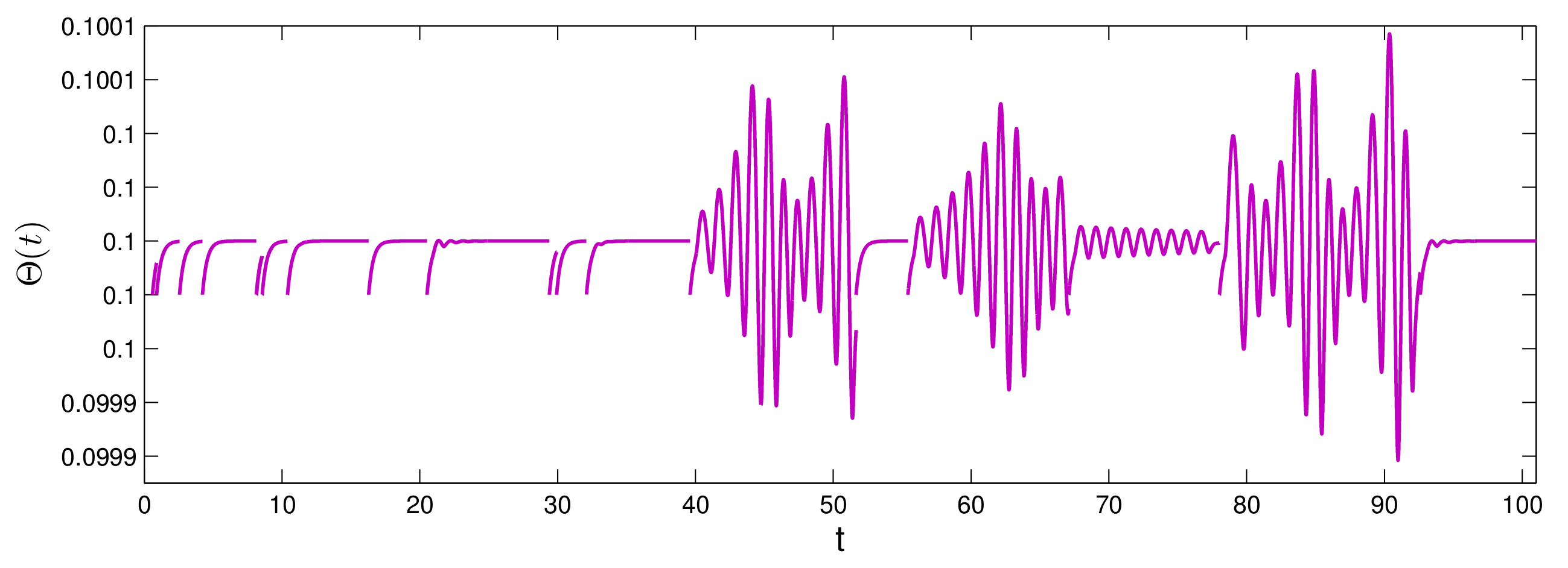
Example 1.

We will construct a Poisson stable function. Consider the logistic equation

$$\begin{array}{c}\hfill {\varpi }_{k + 1} = \mu {\varpi }_k(1 - {\varpi }_k),k\in \mathbb{Z}.\end{array}$$

(16)

in the interval $[0,1]$. For each $\mu \in [3 + {\left(\frac{2}{3}\right)}^{1/2},4]$, the equation has Poisson stable solution ${\tau }_k,k\in \mathbb{Z}$ [23]. That is, there exists a sequence $l_p\to \infty ,p\in \mathbb{N}$, which satisfies $|{\tau }_{k + l_p} - {\tau }_k|\to 0$ as $p\to \infty ,$ for each k in finite set of integers.

First, we specify the discontinuity moments as follows

$$\begin{array}{c}\hfill {\theta }_k = k + {\tau }_k,k\in \mathbb{Z},\end{array}$$

(17)

where ${\tau }_k$, $k\in \mathbb{Z}$ is the Poisson stable solution of (16). Since ${\tau }_k,$ $k\in \mathbb{Z}$ is a Poisson stable sequence, there exists a sequence $l_p\to \infty ,p\in \mathbb{N}$, which satisfies $|{\theta }_{k + l_p} - {\theta }_k|\to 0$ as $n\to \infty$ for each k in bounded intervals of integers.

Let us show that ${\theta }_k,k\in \mathbb{Z}$ is a Poisson stable sequence, with $t_p = l_p$ for each $p\in \mathbb{N}$. We have that

$$\begin{array}{c}\hfill |{\theta }_{k + l_p} - t_p - {\theta }_k| = |k + l_p + {\tau }_{k + l_p} - l_p - k - {\tau }_k| = |{\tau }_{k + l_p} - {\tau }_k|\to 0,\end{array}$$

as $p\to \infty ,$ $k\in \mathbb{Z}$ for each k in finite set of integers.

Consider the following integral equation defined by

$${\displaystyle \mathrm{\Theta }\left(t\right) = {\int }_{-\infty }^t{e}^{ - 3(t - s)}\mathrm{\Omega }\left(s\right)ds,t\in \mathbb{R},}$$

where $\mathrm{\Omega }\left(t\right)$ is a piecewise constant function, which is determined by the equation $\mathrm{\Omega }\left(t\right) = {\tau }_k$ for $t\in [{\theta }_k,{\theta }_{k + 1}),$ $k\in \mathbb{Z}$, on $\mathbb{R}$. $\mathrm{\Theta }\left(t\right)$ is bounded function on the whole real axis which satisfies $\underset{t\in \mathbb{R}}{sup}\left|\mathrm{\Theta }\left(t\right)\right|\le 1/3$ (Figure 1).

Let us check if the function $\mathrm{\Theta }\left(t\right)$ satisfies the Poisson stability condition. Consider a number $ϵ>0$ and a bounded and closed interval $\left[\alpha ,\beta \right]$. Assume, without loss of generality, that α and β are integers. Choose ${\zeta }_{ϵ}>0$ and $\gamma <\alpha ,$ which satisfy $\frac{2}{3}{e}^{ - 3(\alpha - \gamma )}<\frac{ϵ}{3}$, $\frac{1}{3}{\zeta }_{ϵ}\left[1 - e^{ - 3(\beta - \gamma )}\right]<\frac{ϵ}{3}$ and $\frac{2}{3}(e^{3{\zeta }_{ϵ}} - 1)<\frac{ϵ}{3}$, where $\gamma \in \mathbb{Z}$. Moreover, let n be a large natural number such that $|\mathrm{\Omega }(t + t_p) - \left|\mathrm{\Omega }\left(t\right)\right|<{\zeta }_{ϵ}$ on $\left[\gamma ,\beta \right]$.

Then for all $\left[\alpha ,\beta \right]$, we obtain

$$\begin{array}{ccc}& & {\displaystyle |\mathrm{\Theta }(t + t_p) - \mathrm{\Theta }\left(t\right)| = |{\int }_{-\infty }^t{e}^{-3(t - s)}(\mathrm{\Omega }(s + t_p) - \mathrm{\Omega }\left(s\right))ds|}\hfill \\ & & {\displaystyle \hspace{1em}\le |{\int }_{-\infty }^{\gamma }{e}^{-3(t - s)}(\mathrm{\Omega }(s + t_p) - \mathrm{\Omega }\left(s\right))ds|}\hfill \\ & & {\displaystyle \hspace{1em}+|{\int }_{\gamma }^{\beta }{e}^{-3(t - s)}(\mathrm{\Omega }(s + t_p) - \mathrm{\Omega }\left(s\right))ds|}\hfill \\ & & {\displaystyle \hspace{1em}+|\sum _{i^{\prime } = k}^{k + d - 1}\underset{{\theta }_{i^{\prime } + 1}}{\overset{{\theta }_{i^{\prime } + 1 + l_p} - t_p}{\int }}{e}^{-3(t - s)}(\mathrm{\Omega }(s + t_p) - \mathrm{\Omega }\left(s\right))ds|}\hfill \\ & & {\displaystyle \hspace{1em}\le {\int }_{-\infty }^{\gamma }{e}^{-3(t - s)}2ds + {\int }_{\gamma }^{\beta }{e}^{-3(t - s)}{\zeta }_{ϵ}ds + \sum _{i^{\prime } = k}^{k + d - 1}\underset{{\theta }_{i^{\prime } + 1}}{\overset{{\theta }_{i^{\prime } + 1 + l_p} - t_p}{\int }}{e}^{ - 3(t - s)}2ds}\hfill \\ & & \hspace{1em}\le \frac{2}{3}{e}^{ - 3(\alpha - \gamma )} + \frac{1}{3}{\zeta }_{ϵ}[1 - e^{-3(\beta - \gamma )}] + \frac{2}{3}(e^{3{\zeta }_{ϵ}} - 1)\hfill \\ & & \hspace{1em}\le \frac{ϵ}{3} + \frac{ϵ}{3} + \frac{ϵ}{3} = ϵ.\hfill \end{array}$$

Thus, $|\mathrm{\Theta }(t + t_p) - \mathrm{\Theta }\left(t\right)|\to 0$ as $n\to \infty$ uniformly on the interval $\left[\alpha ,\beta \right]$.

Example 2.

Finally, let us consider the SISICNN

$$\begin{array}{c}\hfill \begin{array}{c}{\displaystyle \frac{d{x}_{ij}\left(t\right)}{dt} = a_{ij}{x}_{ij}\left(t\right) - \sum _{C_{hl}\in N_r(i,j)}{C}_{ij}^{hl}f\left(x_{hl}\left(\gamma \left(t\right)\right)\right)x_{ij}\left(t\right) + v_{ij}\left(t\right),t\ne {\theta }_k,}\hfill \\ {\displaystyle \Delta x_{ij}{|}_{t = {\theta }_k} = b_{ij}{x}_{ij}\left({\theta }_k\right) + \sum _{C_{hl}\in N_r(i,j)}{D}_{ij}^{hl}g\left(x_{hl}\left({\theta }_k\right)\right)x_{ij}\left({\theta }_k\right) + h_{ijk},}\hfill \end{array}\end{array}$$

(18)

where $m = 2,n = 3,$ the rates of the cells activity are given as follows: $a_{11} = 0.2$, $a_{12} = - 0.2$, $a_{13} = - 0.1$, $a_{21} = - 0.2$, $a_{22} = 0$, $a_{23} = - 0.1$, $b_{11} = e^{ - 1.2} - 1$, $b_{12} = e^{ - 0.6} - 1$, $b_{13} = e^{ - 0.6} - 1$, $b_{21} = e^{ - 1.8} - 1$, $b_{22} = e^{ - 0.8} - 1$, $b_{23} = e^{ - 1.2} - 1$, and the coupling strength of postsynaptic activity are given by

$$\begin{gathered} \left(\begin{array}{lll}{C}_{ij}^{11}& C_{ij}^{12}& C_{ij}^{13}\\ C_{ij}^{21}& C_{ij}^{22}& C_{ij}^{23}\end{array}\right) = \left(\begin{array}{lll}0.03& 0.07& 0.04\\ 0.02& 0.05& 0.01\end{array}\right), \\ \left(\begin{array}{ccc}{D}_{ij}^{11}& D_{ij}^{12}& D_{ij}^{13}\\ D_{ij}^{21}& D_{ij}^{22}& D_{ij}^{23}\end{array}\right) = \left(\begin{array}{ccc}0.06& 0.03& 0.01\\ 0.09& 0.02& 0.03\end{array}\right) \end{gathered}$$

for each i and j such that the cell $C_{hl}$, $h,l = 1,2,3$, belong to the neighborhood $N_1(i,j)$. As activation and impact activations, we consider the following functions $f\left(s\right) = 0.008arctan\left(\frac{s}{6}\right)$, $g\left(s\right) = 0.005tanh\left(\frac{s}{4}\right)$, and the continuous-impact external inputs are given by

$$\begin{gathered} \left(\begin{array}{lll}{v}_{11}\left(t\right)& v_{12}\left(t\right)& v_{13}\left(t\right)\\ v_{21}\left(t\right)& v_{22}\left(t\right)& v_{23}\left(t\right)\end{array}\right) = \left(\begin{array}{lll}0.32{\mathrm{\Theta }}^3\left(t\right)& 0.48\Theta \left(t\right) - 0.5& 0.27{\mathrm{\Theta }}^3\left(t\right) - 0.1\\ 0.54\Theta \left(t\right)& 0.15{\mathrm{\Theta }}^3\left(t\right) - 0.3& - 0.49\Theta \left(t\right) - 0.2\end{array}\right), \\ \left(\begin{array}{lll}{h}_{11k}\left(t\right)& h_{12k}\left(t\right)& h_{13k}\left(t\right)\\ h_{21k}\left(t\right)& h_{22k}\left(t\right)& h_{23k}\left(t\right)\end{array}\right) = \left(\begin{array}{lll}-0.4{\tau }_k + 0.03& -0.6{\tau }_k^3& 0.5{\tau }_k\\ 0.2{\tau }_k^3 - 0.02& 0.3{\tau }_k& 0.1{\tau }_k\end{array}\right). \end{gathered}$$

The argument function $\gamma \left(t\right) = {\xi }_k$ is defined by the sequence ${\xi }_k = {\theta }_k$, $k\in \mathbb{Z}.$

We checked that conditions $\left(C1\right)$–$\left(C8\right)$ are satisfied for (18) with $K_{ij} = 2.5$, $M_{ij} = 1.26$ for all $i = 1,2,j = 1,2,3$, ${\mathsf{\lambda }}_{11} = - 1$, ${\mathsf{\lambda }}_{12} = - 0.8$, ${\mathsf{\lambda }}_{13} = - 0.7$, ${\mathsf{\lambda }}_{21} = - 2$, ${\mathsf{\lambda }}_{22} = - 0.8$, ${\mathsf{\lambda }}_{23} = - 1.3$, $L = 0.0026$, $M = 0.013$ and $H = 12$. Then there exists the unique discontinuous Poisson stable motion $x\left(t\right)$ of SISICNNs (18). In addition, the asymptotic stability conditions $\left(C9\right)$–$\left(C10\right)$ are valid for this solution.

One cannot simulate Poisson stable solution $x\left(t\right)$ since it is impossible to determine the initial value precisely. Consequently, we will consider solution $\psi \left(t\right)$, with initial values ${\psi }_{11}\left(0\right) = - 0.67$, ${\psi }_{12}\left(0\right) = - 0.43$, ${\psi }_{13}\left(0\right) = 2.56$, ${\psi }_{21}\left(0\right) = 0.25$, ${\psi }_{22}\left(0\right) = - 8.42$, ${\psi }_{23}\left(0\right) = 1.26$. Using (15), one can obtain that $\parallel \psi \left(t\right) - x\left(t\right)\parallel \le e^{ - 1.39t}\parallel x\left(t_0\right) - \psi \left(t_0\right)\parallel$, $t\ge 0$. It means that the difference $x\left(t\right) - \psi \left(t\right)$ is decreasing exponentially. So, the graph of $\psi \left(t\right)$ approaches the discontinuous Poisson stable solution $x\left(t\right)$ of the SISCINN (18), as t increases. Then, we consider the graph of $\psi \left(t\right)$ instead of the curve of the Poisson-stable solution $x\left(t\right)$. The coordinates of the function $\psi \left(t\right)$ are shown in Figure 2 and Figure 3.

4. Discussion

The advantages of the SISICNNs under study lie in the following factors: the impulsive part is symmetrical to the differential equation; the inputs/outputs of the system are Poisson-stable functions and the derivatives of the sequences of discontinuity moments are Poisson stable; and there is a presence of a generalized piecewise constant argument.

It is known that many processes studied in applied sciences are described by differential equations. However, in many phenomena that have a sudden change in state [40,41,42], the situation is completely different. The mathematical models of these processes are impulsive differential equations. Thus, we are to study the dynamics of continuous phenomena with sudden interruptions. There are many weighty theoretical and practical results on impulse differential equations [11,12,13,26,40,41,42]. Previously, many models of impulsive neural networks were considered, where the impulsive parts are analogous to their differential parts [11,12,13,43]. Thus, the study of neural networks, in which the equations for the impulses are of the same structure as differential ones have not been practically considered. In this paper, we have removed the deficiency. The symmetry of the model allows to study in detail the state of the network when sharp jumps occur, which makes it possible to explore complex models of impulsive neural networks. Note that such symmetry of the impulsive part can be used not only for SICNNs, but also for impulse models of neural networks of the Hopfield type, neural networks of the Cohen–Grossberg type and those of the inertial type.

In this paper, by continuing the line of new types of oscillations for impulsive models of neural networks, we considered the discontinuous Poisson stable motions of SISICNNs. Poisson stable and unpredictable motions of SICNNs have been researched in several papers and books [20,21,22,23,24,25]. However, neural networks with impacts have not been considered for Poisson stability yet.

Differential equations with piecewise constant argument [26,35,36] occupy an intermediate position between ordinary and functional differential equations. There are many significant results for neural networks, which are separately either impulsive differential equations [11,12,13,14,15,16] and equations with generalized piecewise constant arguments [27]. In this paper, SICNNs were investigated with both impulses and piecewise constant argument.

5. Conclusions

The paper proceeds with the research of oscillations in neural networks and considers Poisson stability. The principal novelty is that the SICNN is symmetrical. That is, the structure of the impulsive part is analogous to the differential equation since circuits for electrical processes happen shortly and have to mimic those with continuous time.

The new model as well as the type of recurrence provide challenges in the analysis of the neural networks and proving of Poisson stability. Moreover, additional complexity in the research is caused by the discontinuous argument. Conditions for the existence of Poisson-stable discontinuous motions of SISICNNs are obtained.

The results can be effectively used in parallel image and signal processing, pattern recognition [3,4,5,7,8,9,10], and different problems of control and synchronization in deterministic and stochastic processes [49,50,51].

References

1. Chua, L.O.; Yang, L. Cellular neural networks: Theory. IEEE Trans. Circuits Syst. 1988, 35, 1257–1272. [Google Scholar] [CrossRef]
2. Chua, L.O.; Yang, L. Cellular neural networks: Applications. IEEE Trans. Circuits Syst. 1988, 35, 1273–1299. [Google Scholar] [CrossRef]
3. Ando, T.; Uwate, Y.; Nishio, Y. Image Processing by Cellular Neural Networks with Switching Two Templates. In Proceedings of the IEEE Asia Pacific Conference on Postgraduate Research in Microelectronics and Electronics (PrimeAsia’17), Kuala Lumpur, Malaysia, 31 October–2 November 2017; pp. 45–48. [Google Scholar]
4. Chua, L.O.; Yang, L.; Krieg, K.R. Signal Processing Using Cellular Neural Networks. In Parallel Processing on VLSI Arrays; Nossek, J.A., Ed.; Springer: Boston, MA, USA, 1991. [Google Scholar]
5. Huang, K.; Hsieh, W. Seismic pattern recognition using cellular neural network. In Proceedings of the 2017 IEEE International Geoscience and Remote Sensing Symposium (IGARSS), Fort Worth, TX, USA, 23–28 July 2017; pp. 3712–3715. [Google Scholar]
6. Bouzerdoum, A.; Pinter, R.B. Shunting inhibitory cellular neural networks: Derivation and stability analysis. IEEE Trans. Circuits Syst.-I Fund. Theory Appl. 1993, 40, 215–221. [Google Scholar] [CrossRef]
7. Bouzerdoum, A.; Pinter, R.B. Nonlinear lateral inhibition applied to motion detection in the fly visual system. In Nonlinear Vision: Determination of Neural Receptive Fields, Function, and Networks; Pinter, R.B., Nabet, B., Eds.; CRC Press: Boca Raton, FL, USA, 1992; pp. 423–450. [Google Scholar]
8. Carpenter, G.A.; Grossberg, S. The ART of adaptive pattern recognition by a self-organizing neural network. Computer 1988, 21, 77–88. [Google Scholar] [CrossRef]
9. Cheung, H.N.; Bouzerdoum, A.; Newland, W. Properties of shunting inhibitory cellular neural networks for colour image enhancement. In Proceedings of the 6th International Conference on Neural Information Processing, Perth, Australia, 16–20 November 1999; pp. 1219–1223. [Google Scholar]
10. Jernigan, M.E.; McLean, G.F. Lateral inhibition and image processing. In Nonlinear Vision: Determination of Neural Receptive Fields, Function, and Networks; Pinter, R.B., Nabet, B., Eds.; CRC Press: Boca Raton, FL, USA, 1992; pp. 451–462. [Google Scholar]
11. Gui, Z.; Ge, W. Periodic solution and chaotic strange attractor for shunting inhibitory cellular neural networks with impulses. Chaos 2006, 16, 033116. [Google Scholar] [CrossRef]
12. Xia, Y.; Cao, J.; Huang, Z. Existence and exponential stability of almost periodic solution for shunting inhibitory cellular neural networks with impulses. Chaos Solitons Fractals 2007, 34, 1599–1607. [Google Scholar] [CrossRef]
13. Li, Y.; Shu, J. Anti-periodic solutions to impulsive shunting inhibitory cellular neural networks with distributed delays on time scales. Commun. Nonlinear Sci. Numer. Simul. 2011, 16, 3326–3336. [Google Scholar] [CrossRef]
14. Akça, H.; Alassar, R.; Covachev, V.; Covacheva, Z.; Al-Zahrani, E. Continuous-time additive Hopfield-type neural networks with impulses. J. Math. Anal. Appl. 2004, 290, 436–451. [Google Scholar] [CrossRef]
15. Stamov, G.T.; Stamova, I.M. Almost periodic solutions for impulsive neural networks with delay. Appl. Math. Model. 2007, 31, 1263–1270. [Google Scholar] [CrossRef]
16. Pinto, M.; Robledo, G. Existence and stability of almost periodic solutions in impulsive neural network models. Appl. Math. Comput. 2010, 217, 4167–4177. [Google Scholar] [CrossRef]
17. Poincaré, H. Les Methodes Nouvelles de la Mecanique Celeste; Gauthier-Villars: Paris, France, 1892; Volume I–II. [Google Scholar]
18. Poincaré, H. Les Methodes Nouvelles de la Mecanique Celeste; Gauthier-Villars: Paris, France, 1899; Volume III. [Google Scholar]
19. Birkhoff, G.D. Dynamical Systems; American Mathematical Society: Providence, RI, USA, 1927. [Google Scholar]
20. Akhmet, M.; Tleubergenova, M.; Zhamanshin, A. Quasilinear differential equations with strongly unpredictable solutions. Carpathian J. Math. 2020, 36, 341–3494. [Google Scholar] [CrossRef]
21. Akhmet, M.; Seilova, R.; Tleubergenova, M.; Zhamanshin, A. Shunting inhibitory cellular neural networks with strongly unpredictable oscillations. Commun. Nonlinear Sci. Numer. Simulat. 2020, 89, 05287. [Google Scholar] [CrossRef]
22. Akhmet, M.; Tleubergenova, M.; Nugayeva, Z. Unpredictable solutions of impulsive quasi-linear systems. Discontin. Nonlinearity Complex. 2022, 11, 73–89. [Google Scholar] [CrossRef]
23. Akhmet, M.; Tleubergenova, M.; Zhamanshin, A. Modulo periodic Poisson stable solutions of quasilinear differential equations. Entropy 2021, 23, 1535. [Google Scholar] [CrossRef] [PubMed]
24. Akhmet, M.; Tleubergenova, M.; Zhamanshin, A. Dynamics of shunting Inhibitory cellular neural networks with variable two-component passive decay rates and Poisson Stable inputs. Symmetry 2022, 14, 1162. [Google Scholar] [CrossRef]
25. Akhmet, M.U. Domain Structured Dynamics: Unpredictability, Chaos Randomness, Fractals, Differential Equations and Neural Networks; IOP Publishing: Bristol, UK, 2021. [Google Scholar]
26. Akhmet, M.U. Almost Periodicity, Chaos, and Asymptotic Equivalence; Springer: New York, NY, USA, 2020. [Google Scholar]
27. Wan, L.; Wu, A. Stabilization control of generalized type neural networks with piecewise constant argument. J. Nonlinear Sci. Appl. 2016, 9, 3580–3599. [Google Scholar] [CrossRef]
28. Sell, G.R. Topological Dynamics and Ordinary Differential Equations; Van Nostrand Reinhold Company: London, UK, 1971. [Google Scholar]
29. Akhmet, M. Principles of Discontinuous Dynamical Systems; Springer: New York, NY, USA, 2010. [Google Scholar]
30. Akhmet, M.; Fen, M.O. Unpredictable points and chaos. Commun. Nonlinear Sci. Numer. Simulat. 2016, 40, 1–5. [Google Scholar] [CrossRef]
31. Shcherbakov, B.A. Classification of Poisson-stable motions. Pseudo-recurrent motions. Dokl. Akad. Nauk SSSR 1962, 146, 322–324. (In Russian) [Google Scholar]
32. Shcherbakov, B.A. Topologic Dynamics and Poisson Stability of Solutions of Differential Equations; Stiinta: Chisinau, Moldova, 1972. (In Russian) [Google Scholar]
33. Shcherbakov, B.A. Poisson Stability of Motions of Dynamical Systems and Solutions of Differential Equations; Stiinta: Chisinau, Moldova, 1985. (In Russian) [Google Scholar]
34. Cheban, D.; Liu, Z. Poisson stable motions of monotone nonautonomus dynamical systems. Sci. China Math. 2019, 62, 1391–1418. [Google Scholar] [CrossRef]
35. Akhmet, M.U. On the integral manifolds of the differential equations with piecewise constant argument of generalized type. In Proceedings of the Conference on Differential and Difference Equations at the Florida Institute of Technology, Melbourne, FL, USA, 1–5 August 2005; pp. 11–20. [Google Scholar]
36. Akhmet, M.U. Integral manifolds of differential equations with piecewise constant argument of generalized type. Nonlinear Anal. 2007, 66, 367–383. [Google Scholar] [CrossRef]
37. Castillo, S.; Pinto, M. Existence and stability of almost periodic solutions to differential equations with piecewise constant argument. Electron. J. Differ. Equ. 2015, 58, 1–15. [Google Scholar]
38. Coronel, A.; Maulén, C.; Pinto, M.; Sepúlveda, D. Dichotomies and asymptotic equivalence in alternately advanced and delayed differential systems. J. Math. Anal. Appl. 2017, 450, 1434–1458. [Google Scholar] [CrossRef]
39. Zou, C.; Xia, Y.; Pinto, M.; Shi, J.; Bai, Y. Boundness and linearization of a class of differential equations with piecewise constant argument. Qual. Theory Dyn. Syst. 2019, 18, 495–531. [Google Scholar] [CrossRef]
40. Girel, S.; Crauste, F. Existence and stability of periodic solutions of an impulsive differential equation and application to CD8 T-cell differentiation. J. Math. Biol. 2018, 76, 1765–1795. [Google Scholar] [CrossRef] [PubMed]
41. Ghosh, P.; Peters, J.F. Impulsive differential equation model in methanol poisoning detoxification. J. Math. Chem. 2020, 58, 126–145. [Google Scholar] [CrossRef]
42. Zhao, Z.; Li, Q.; Chen, L. Effect of rhizosphere dispersal and impulsive input on the growth of wetland plant. Math. Comput. Simul. 2018, 152, 69–80. [Google Scholar] [CrossRef]
43. Li, K.; Zhang, X.; Li, Z. Global exponential stability of impulsive cellular neural networks with time-varying and distributed delay. Chaos Solitons Fractals 2009, 41, 1427–1434. [Google Scholar] [CrossRef]
44. Li, Y.; Liu, C.; Zhu, L. Global exponential stability of periodic solution for shunting inhibitory CNNs with delays. Phys. Lett. A 2005, 337, 46–54. [Google Scholar] [CrossRef]
45. Khan, A.; Salahuddin, S. Negative capacitance in ferroelectric materials and implications for steep transistors. In Proceedings of the 2015 IEEE SOI-3D-Subthreshold Microelectronics Technology Unified Conference (S3S), Rohnert Park, CA, USA, 5–8 October 2015; pp. 1–3. [Google Scholar]
46. Khan, A.I.; Chatterjee, K.; Duarte, J.P.; Lu, Z.; Sachid, A.; Khandelwal, S.; Ramesh, R.; Hu, C.; Salahuddin, S. Negative capacitance in short-channel finfets externally connected to an epitaxial ferroelectric capacitor. IEEE Electron Device Lett. 2016, 37, 111–114. [Google Scholar] [CrossRef]
47. Si, M.; Su, C.-J.; Jiang, C.; Conrad, N.; Zhou, H.; Maize, K.; Qiu, G.; Wu, C.-T.; Shakouri, A.; Alam, M.; et al. Steep-slope hysteresis-free negative capacitance mos2 transistors. Nat. Nanotechnol. 2018, 13, 24–28. [Google Scholar] [CrossRef]
48. Akhmet, M.; Erim, G. Almost Periodic Solutions of Recurrently Structured Impulsive Neural Networks. Discontin. Nonlinearity Complex. 2022, 11, 373–385. [Google Scholar] [CrossRef]
49. Zhu, Q.; Cao, J. Stability analysis of Markovian jump stochastic BAM neural networks with impulse control and mixed time delays. IEEE Trans. Neural. Netw. Learn. Syst. 2012, 23, 467–479. [Google Scholar] [PubMed]
50. Zhu, Q. Stabilization of Stochastic Nonlinear Delay Systems With Exogenous Disturbances and the Event-Triggered Feedback Control. IEEE Trans. Autom. Control. 2019, 64, 3764–3771. [Google Scholar] [CrossRef]
51. Ding, K.; Zhu, Q. A Note on Sampled-Data Synchronization of Memristor Networks Subject to Actuator Failures and Two Different Activations. IEEE Trans. Circuits Syst. II Express Briefs 2021, 68, 2097–2101. [Google Scholar] [CrossRef]
Figure 1. Discontinuous Poisson stable function Θ ( t ) .
Symmetry 14 01754 g001
Figure 2. Coordinates of ψ ( t ) , which converges to the Poisson stable solution x ( t ) of the SISICNN (18).
Symmetry 14 01754 g002
Figure 3. The ψ 1     ψ 2     ψ 3 and ψ 4     ψ 5     ψ 6 space coordinates of ψ ( t ) , which converges to the Poisson stable solution x ( t ) of the SISICNN (18).
Symmetry 14 01754 g003
Publisher’s Note: MDPI stays neutral with regard to jurisdictional claims in published maps and institutional affiliations.