Analysis of Drill-String Nonlinear Dynamics Using the Lumped-Parameter Method

Abstract

This work aims at studying the nonlinear dynamics of drill strings using the lumped-parameter method (LPM). The study is based on the good consistency of the results of the test problem where the model of the longitudinal vibrations of a horizontal drill string with a static compressive load at the left end is considered. In this paper, this method is applied to discretize linear and nonlinear models of the lateral vibrations of a vertical drill string under the effect of a supersonic gas flow. The obtained results are verified with the previously published data. The optimal number of the drill-string partitions is determined using the developed application, which allows us to estimate the accuracy of the loaded data. The numerical solution of the model is obtained using the fourth-order Runge–Kutta method. The optimization of the numerical algorithm using parallel-programming tools is carried out, and the efficiency of the method is analyzed.

1. Introduction

The need to improve the dynamic characteristics of industrial mechanisms and increase their reliability makes the problem of machine dynamics, in particular, the equipment of the oil and gas industry, one of the most relevant [1,2]. However, the technological complexity and high nonlinearity of the investigated phenomena significantly complicate the modeling process, which requires the introduction of certain simplifications and assumptions in the models.

In the literature, the dynamic models based on the Euler–Bernoulli beam systems, such as [3,4,5], Timoshenko beams [6,7] and the mathematical models of drill-string linear vibrations developed by V.I. Gulyaev et al. [8,9], are widely presented. Nevertheless, the field of application of linear models is rather limited, since the excessive idealization of the studied phenomena allows only special cases to be included and the process might be described inadequately. This explains the interest of many authors in the study of nonlinearity.

Several works are devoted to the modeling of nonlinear dynamic systems. V.I. Erofeev [10] reviewed the results of studies of nonlinear wave processes in rod systems and concluded that it was necessary to use higher approximation theories that took into account geometric and physical nonlinearities in order to avoid the accumulation of distortions that significantly affected the wave fronts. In [11,12], mathematical models were presented in nonlinear formulations and derived using the Ostrogradsky–Hamilton variation method; in addition, the comparative analysis with classical linear models was carried out. In [11], the case of the contact interaction between a drill string and borehole walls, based on the Hertz contact law, was considered; in [12], the authors concluded that nonlinear models were more stable in comparison with linear ones and that there was a significant difference in the dynamic characteristics of these models, which increased with the decrease in Young’s modulus and the increase in the acceleration. Q. Yan et al. [13] investigated the nonlinear dynamics of a viscoelastic Timoshenko beam under parametric excitation caused by external harmonic vibrations. To obtain a solution, the four-term Bubnov–Galerkin method combined with Runge–Kutta time discretization was utilized. The analysis showed the effect of the forced oscillation amplitude on the nonlinear dynamic response of the beam. The vibration characteristics of the drill string during gas drilling were considered by X.P. Chang et al. [14]. In [15], using an analytical model for predicting lateral vibrations, the dynamic stability of the drill string was investigated, and the primary and secondary instabilities were found using the Bolotin method. F. Bakhtiari-Nejad and A. Hosseinzadeh [16] studied the dynamic stability of the coupled axial and torsional motion of the drill string using the semi-discretization method.

To remove restrictions on the performance of drilling operations, composite drill strings and high-tech rotors with complex dynamic characteristics have been developed in recent years. Amongst the works devoted to this topic, it is worth noting the work of M. Mohammadzadeh et al. [17], where the authors investigated fully coupled nonlinear vibrations of a composite drill string consisting of orthotropic layers using the Lagrangian approach and the finite element method and conducted a comparative analysis on a steel drill string.

In [18,19], the authors studied the nonlinear spatial vibrations of a drill string in gas and liquid flows. In view of the poorly studied nonlinear problems of mechanism dynamics, including drill strings, the search and application of the most effective modeling methods are of scientific and practical interest. Amongst modern approaches, one of the most widespread method is the Ostrogradsky–Hamilton variation method used for deriving models based on the V.V. Novozhilov nonlinear theory of finite deformations [11], the Euler–Bernoulli beam theory and the von Kármán nonlinear strain theory [12]; the Bubnov–Galerkin method is mainly utilized before implementing the numerical solution [12,13,14,15].

The purpose of this work is the application of the lumped-parameter method (LPM) for solving drilling problems and the assessment of its effectiveness. The essence of the LPM is to reduce the continuity equation to its discrete analogue by approximating the spatial components, that is, each link is represented as a one-dimensional bar element divided into a finite number of point masses. It is worth noting that for any section, there is a concentration of mass on the neutral axis at the midpoint of the section length, which in total means that the mass conservation law holds. In this paper, the attention is focused on the mathematical side of the issue of the drill string discretization using the LPM and solving the problems of numerical implementation for the system of multiple nonlinear equations to improve the accuracy of the solution.

The LPM was first utilized by J.P. Sadler in the 1970s to study the dynamics of nonlinear elastic multi-link mechanisms [20]. The work was further expanded in [21,22,23]. The LPM is a special case of the finite element method, according to which the dimension of the system decreases, and the basic equation reduces to the system of ODEs. This method is widely used in structural mechanics when modeling flat crank mechanisms [24,25,26] and is most justified when studying the dynamics of structures made of dissimilar materials, complicated by non-uniform loading and for nonlinear systems with variable structure.

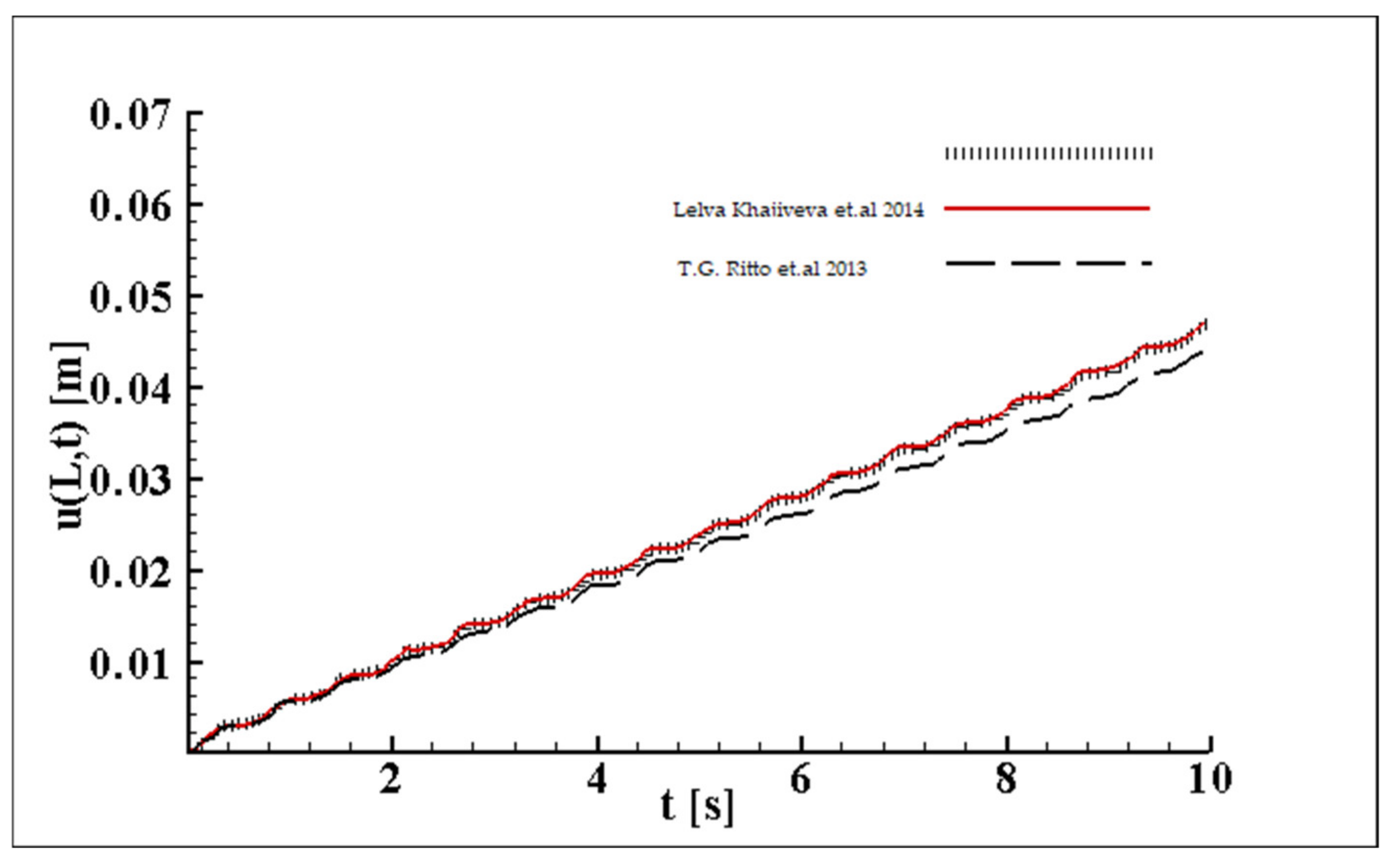
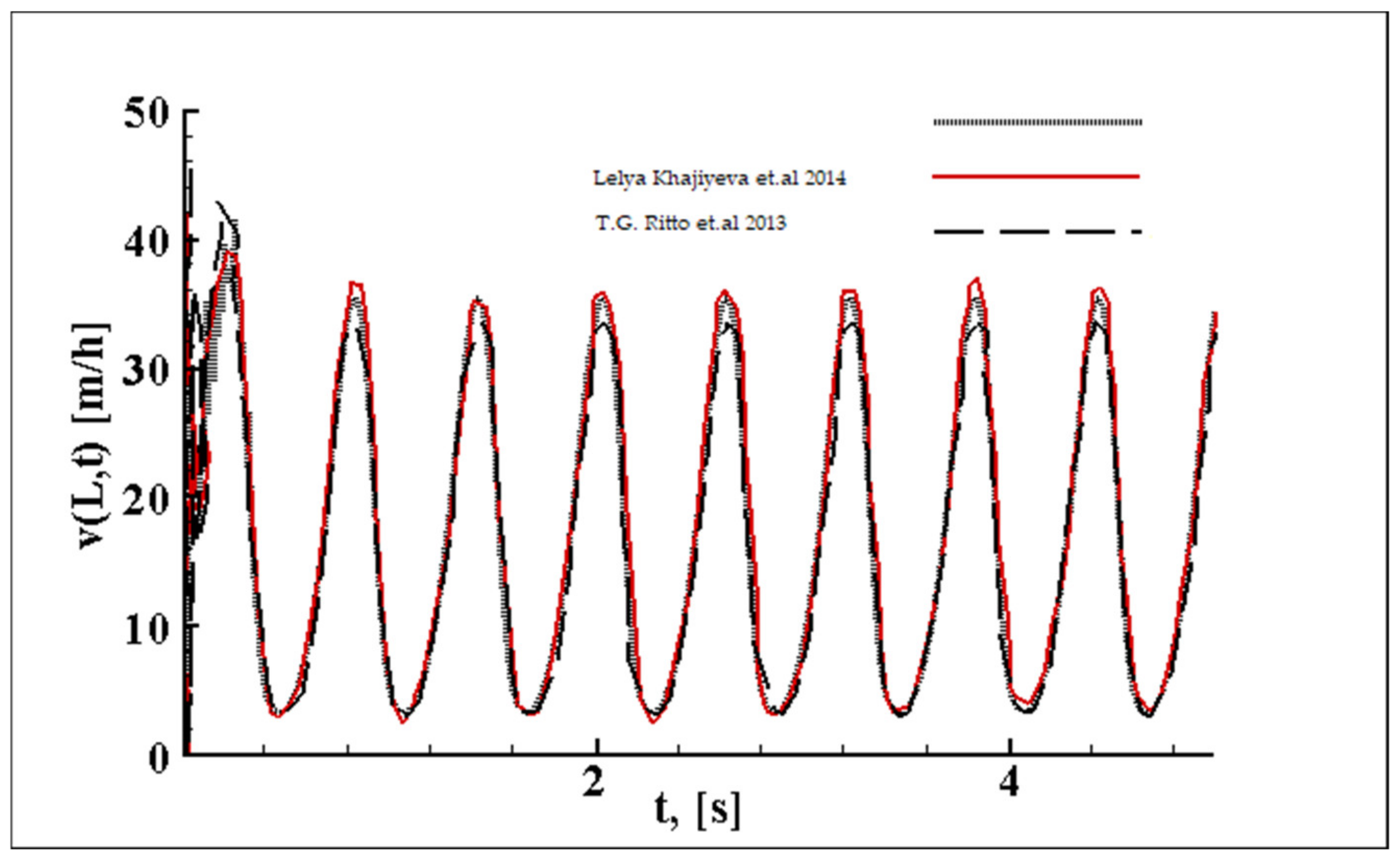
The study of the LPM effectiveness starts with solving a test problem where longitudinal vibrations of a horizontal drill string with a static compressive load at the left end are considered. The model of the horizontal drill-string vibrations is based on that from the work of [27]. T.G. Ritto et al. [28,29] investigated the influence of stochastic processes on the dynamics of a drilling rig when modeling the horizontal drill-string motion. This problem was successfully solved using the lumped-parameter method in [30]. Their research study was expanded by the authors of the current work (see Appendix A). The good consistency of the obtained results of the test problem with the previously published data is the main reason for the continuation of using the LPM for solving drilling problems.

In this paper, the lateral vibrations of a vertical drill string taking into account the influence of the environmental factors are considered. The study of lateral vibrations is of great interest, since this type of vibrations is more destructive in nature in comparison with axial and torsional ones and may cause equipment breakdown and accidents while drilling [31].

2. Mathematical Model

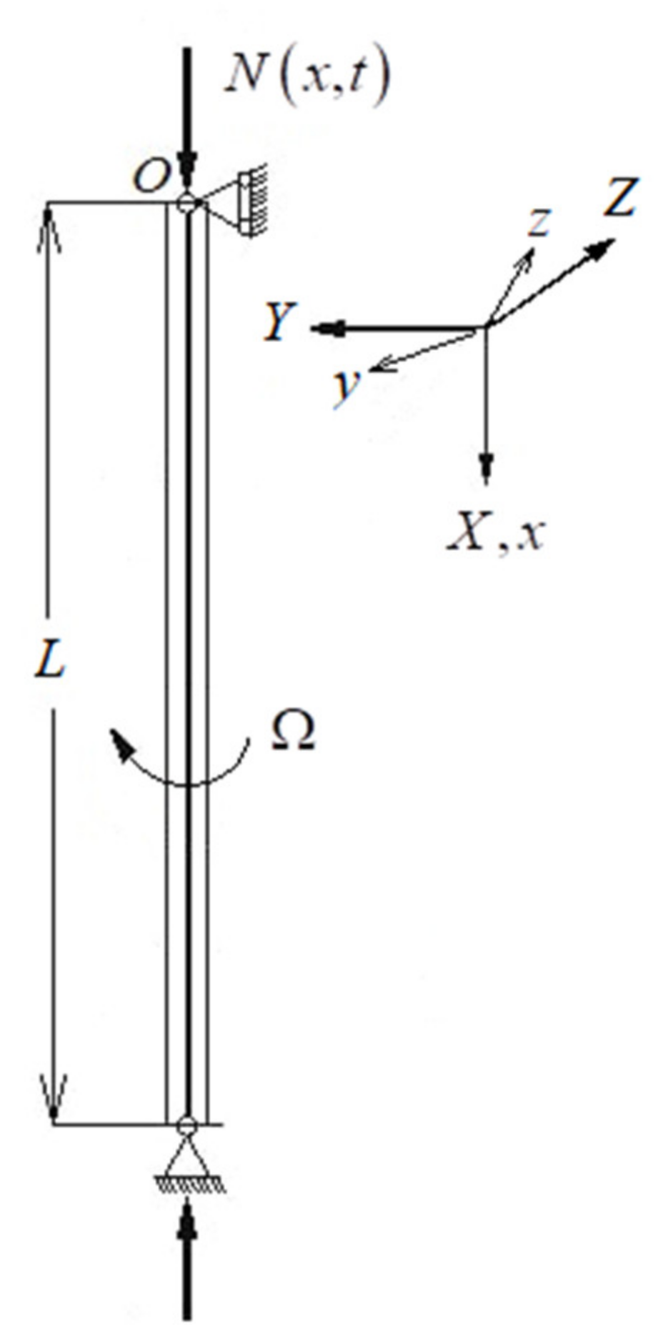
Consider a drill string under the action of an external load transmitted from a drilling rig when interacting with the environment in the process of shallow drilling. The sketch of the drill string modeled as an elastic rod rotating around the x-axis with angular speed $\Omega$ and being under the action of an axial compressive load $N(x,t)$ is shown in Figure 1.

The nonlinear mathematical model of lateral vibrations of the vertical drill string under the action of a gas flow moving at supersonic speed is under consideration (see [19] for more details):

$$\begin{array}{l}\rho A\frac{{\partial }^{2}u}{\partial t^2}+EI\frac{{\partial }^{4}u}{\partial x^4}-\rho I\frac{{\partial }^{4}u}{\partial t^2\partial x^2}+\frac{\partial }{\partial x}\left(N(x,t)\frac{\partial u}{\partial x}\right)-\frac{EA}{1-\nu }\frac{\partial }{\partial x}{\left(\frac{\partial u}{\partial x}\right)}^3-\rho A{\Omega }^{2}u\\ -h{P}_0\kappa \left(\overline{M}\frac{\partial u}{\partial x}-\frac{\kappa +1}{4}{\overline{M}}^2{\left(\frac{\partial u}{\partial x}\right)}^2+\frac{\kappa +1}{12}{\overline{M}}^3{\left(\frac{\partial u}{\partial x}\right)}^3\right)=0,\end{array}$$

(1)

where $u(x,t)$ is the lateral displacement of the drill string, $\rho$ is the density of the drill-string material, $A$ is the cross-section area, $E$ is Young’s modulus, $I$ is the inertia moment of the drill-string cross-section, $N(x,t)$ is the axial compressive load, $\nu$ is Poisson’s ratio, $\Omega$ is the angular speed of rotation of the drill string, $\kappa$ is the polytropic exponent, $\overline{M}$ is the Mach number, $P_0$ is the pressure of the unperturbed gas flow and $h$ is the drill-string wall thickness.

The reason for studying plane vibrations of the drill string in the paper is the fact that the nature of the drill string spatial vibrations is similar for both spatial displacement components with slight difference in their vibration periods and maximum amplitudes as obtained in [32].

The boundary conditions corresponding to the simply supported rod are represented as follows:

$$\begin{array}{l}u(x,t)=0,\hspace{1em}EI\frac{{\partial }^{2}u(x,t)}{\partial x^2}=0\hspace{1em}\mathrm{for}\hspace{1em}x=0,\\ u(x,t)=0,\hspace{1em}EI\frac{{\partial }^{2}u(x,t)}{\partial x^2}=0\hspace{1em}\mathrm{for}\hspace{1em}x=L,\end{array}$$

(2)

where $L$ is the drill-string length.

The initial conditions are given by:

$$\begin{array}{l}u(x,t)=0\hspace{1em}\left(0\le x\le L\right),\\ \frac{\partial u(x,t)}{\partial t}=C_1\hspace{1em}\left(0<x<L\right)\hspace{1em}\mathrm{for}\hspace{1em}t=0,\end{array}$$

(3)

where $C_1$ is a constant determining the displacement speed of the drill-string cross-section at the initial moment of time from the initial position.

The geometrically linear model of the drill-string lateral vibrations is also considered to study the need for the application of the nonlinear model, as well as to analyze the behavior of the LPM for various systems describing the drilling processes. For the geometrically linear model, nonlinear term $-\frac{EA}{1-\nu }\frac{\partial }{\partial x}{\left(\frac{\partial u}{\partial x}\right)}^3$ is taken to be zero, but the nonlinearity from the gas flow term is preserved, i.e.,:

$$\begin{array}{l}\rho A\frac{{\partial }^{2}u}{\partial t^2}+EI\frac{{\partial }^{4}u}{\partial x^4}-\rho I\frac{{\partial }^{4}u}{\partial t^2\partial x^2}+\frac{\partial }{\partial x}\left(N(x,t)\frac{\partial u}{\partial x}\right)-\rho A{\Omega }^{2}u\\ -h{P}_0\kappa \left(\overline{M}\frac{\partial u}{\partial x}-\frac{\kappa +1}{4}{\overline{M}}^2{\left(\frac{\partial u}{\partial x}\right)}^2+\frac{\kappa +1}{12}{\overline{M}}^3{\left(\frac{\partial u}{\partial x}\right)}^3\right)=0\end{array}$$

(4)

with boundary and initial conditions (2) and (3).

3. Model Discretization by LPM

The lumped-parameter method (LPM) is applied to find the numerical solution of models (1) and (4) with conditions (2) and (3). The drill string modeled as a one-dimensional rod element is split into a finite number of line segments of length $2l=\frac{L}{N-1}$, where $N$ is the number of partition points. Then, the considered equation of motion and boundary conditions are approximated with respect to the spatial variable using discrete formulas.

The following metric in spatial and time variables is introduced to make the system dimensionless (sign ∼ is further omitted):

$$u=L\tilde{u},\hspace{1em}x=L\tilde{x},\hspace{1em}t=\frac{\tilde{t}}{c},\hspace{1em}c=\sqrt{\frac{E}{\rho L^2}}.$$

(5)

Substituting (5) in (1)–(3) and assuming axial load $N(x,t)$ to be constant, namely, $N(x,t)=\overline{N}$, we obtain the nonlinear model of the drill-string vibrations in dimensionless variables:

$$\begin{array}{l}\rho AL{c}^2\frac{{\partial }^{2}u}{\partial t^2}+\frac{EI}{L^3}\frac{{\partial }^{4}u}{\partial x^4}-\frac{\rho I{c}^2}{L}\frac{{\partial }^{4}u}{\partial t^2\partial x^2}+\overline{N}\frac{{\partial }^{2}u}{\partial x^2}-\frac{3EA}{(1-\nu )L}{\left(\frac{\partial u}{\partial x}\right)}^2\frac{{\partial }^{2}u}{\partial x^2}-\rho A{\Omega }^{2}Lu\\ -h{P}_0\kappa \left(\overline{M}\frac{\partial u}{\partial x}-\frac{\kappa +1}{4}{\overline{M}}^2{\left(\frac{\partial u}{\partial x}\right)}^2+\frac{\kappa +1}{12}{\overline{M}}^3{\left(\frac{\partial u}{\partial x}\right)}^3\right)=0\end{array}$$

(6)

with boundary conditions:

$$\begin{array}{l}u(x,t)=0,\hspace{1em}\frac{EI}{L}\frac{{\partial }^{2}u(x,t)}{\partial x^2}=0\hspace{1em}\mathrm{for}\hspace{1em}x=0,\\ u(x,t)=0,\hspace{1em}\frac{EI}{L}\frac{{\partial }^{2}u(x,t)}{\partial x^2}=0\hspace{1em}\mathrm{for}\hspace{1em}x=1.\end{array}$$

(7)

The initial conditions are defined as:

$$\begin{array}{l}u(x,t)=0\hspace{1em}\left(0\le x\le 1\right),\\ \frac{\partial u(x,t)}{\partial t}=\frac{C_1}{Lc}\hspace{1em}\left(0<x<1\right)\hspace{1em}\mathrm{for}\hspace{1em}t=0.\end{array}$$

(8)

The geometrically linear model of the drill-string lateral vibrations takes the form:

$$\begin{array}{l}\rho AL{c}^2\frac{{\partial }^{2}u}{\partial t^2}+\frac{EI}{L^3}\frac{{\partial }^{4}u}{\partial x^4}-\frac{\rho I{c}^2}{L}\frac{{\partial }^{4}u}{\partial t^2\partial x^2}+\overline{N}\frac{{\partial }^{2}u}{\partial x^2}-\rho A{\Omega }^{2}Lu\\ -h{P}_0\kappa \left(\overline{M}\frac{\partial u}{\partial x}-\frac{\kappa +1}{4}{\overline{M}}^2{\left(\frac{\partial u}{\partial x}\right)}^2+\frac{\kappa +1}{12}{\overline{M}}^3{\left(\frac{\partial u}{\partial x}\right)}^3\right)=0,\end{array}$$

(9)

where the boundary and initial conditions are given in forms (7) and (8), respectively.

The impact of the drill string own weight considered as a function of its position in the axial load was studied in [32]. Buckling in the drill string bottom part, where the weight attained its maximum value, with a significant rise in the vibration amplitude was revealed.

After discretizing system (6)–(8) with respect to spatial variables on a regular grid, we have:

$$\begin{array}{l}\rho AL{c}^2{\left(\frac{{\partial }^{2}u}{\partial t^2}\right)}_j+\frac{EI}{L^3}\left(\frac{u_{j-2}-4u_{j-1}+6u_j-4u_{j+1}+u_{j+2}}{\Delta x^4}\right)\\ -\frac{\rho I{c}^2}{\Delta x^{2}L}\left({\left(\frac{{\partial }^{2}u}{\partial t^2}\right)}_{j+1}-2{\left(\frac{{\partial }^{2}u}{\partial t^2}\right)}_j+{\left(\frac{{\partial }^{2}u}{\partial t^2}\right)}_{j-1}\right)\\ +\overline{N}\left(\frac{u_{j-1}-2u_j+u_{j+1}}{\Delta x^2}\right)-\frac{3EA}{\left(1-\nu \right)L}{\left(\frac{u_{j+1}-u_{j-1}}{2\Delta x}\right)}^2\left(\frac{u_{j-1}-2u_j+u_{j+1}}{\Delta x^2}\right)-\rho A{\Omega }^{2}L{u}_j\\ -h{P}_0\kappa \left(\overline{M}\left(\frac{u_{j+1}-u_{j-1}}{2\Delta x}\right)-\frac{\kappa +1}{4}{\overline{M}}^2{\left(\frac{u_{j+1}-u_{j-1}}{2\Delta x}\right)}^2+\frac{\kappa +1}{12}{\overline{M}}^3{\left(\frac{u_{j+1}-u_{j-1}}{2\Delta x}\right)}^3\right)=0,\hspace{1em}\\ j=2,\dots ,N-3,\end{array}$$

(10)

$$u_0=0,\hspace{1em}{u}_{N-1}=0,$$

(11)

$$\frac{EI}{L}\frac{u_0-2u_1+u_2}{\Delta x^2}=0,\hspace{1em}\frac{EI}{L}\frac{u_{N-3}-2u_{N-2}+u_{N-1}}{\Delta x^2}=0,$$

(12)

$$t=0:\hspace{1em}u=0,\hspace{1em}\frac{\partial u}{\partial t}=\frac{C_1}{Lc}.$$

(13)

where $N$ is the number of the drill-string partitions,$\Delta x$ is the spatial step ($\Delta x=\frac{L}{N-1}$) and $u_j=u(x_j,t)$.

Accelerations at points $j=1$ and $j=N-2$ are found from boundary conditions (12) and are defined as:

$$\begin{array}{l}\frac{{\partial }^2{u}_1^n}{\partial t^2}=\frac{u_2^n-2u_1^n}{\Delta t^2},\\ \frac{{\partial }^2{u}_{N-2}^n}{\partial t^2}=\frac{u_{N-3}^n-2u_{N-2}^n}{\Delta t^2}.\end{array}$$

(14)

The nonlinear model of the vertical drill-string vibrations takes the form:

$$j=0:\hspace{1em}{\left(\frac{{\partial }^{2}u}{\partial t^2}\right)}_0=0,\hspace{1em}j=1:\hspace{1em}{\left(\frac{{\partial }^{2}u}{\partial t^2}\right)}_1=L{c}^2\frac{u_2-2u_1}{\Delta t^2},$$

(15)

$$\begin{array}{l}j=\overline{2,N-3}:\hspace{1em}\rho AL{c}^2{\left(\frac{{\partial }^{2}u}{\partial t^2}\right)}_j+\frac{EI}{L^3}\left(\frac{u_{j-2}-4u_{j-1}+6u_j-4u_{j+1}+u_{j+2}}{\Delta x^4}\right)\\ -\frac{\rho I{c}^2}{\Delta x^{2}L}\left({\left(\frac{{\partial }^{2}u}{\partial t^2}\right)}_{j+1}-2{\left(\frac{{\partial }^{2}u}{\partial t^2}\right)}_j+{\left(\frac{{\partial }^{2}u}{\partial t^2}\right)}_{j-1}\right)+\overline{N}\left(\frac{u_{j-1}-2u_j+u_{j+1}}{\Delta x^2}\right)\\ -\frac{3EA}{\left(1-\nu \right)L}{\left(\frac{u_{j+1}-u_{j-1}}{2\Delta x}\right)}^2\left(\frac{u_{j-1}-2u_j+u_{j+1}}{\Delta x^2}\right)-\rho A{\Omega }^{2}L{u}_j\\ -h{P}_0\kappa \left(\overline{M}\left(\frac{u_{j+1}-u_{j-1}}{2\Delta x}\right)-\frac{\kappa +1}{4}{\overline{M}}^2{\left(\frac{u_{j+1}-u_{j-1}}{2\Delta x}\right)}^2+\frac{\kappa +1}{12}{\overline{M}}^3{\left(\frac{u_{j+1}-u_{j-1}}{2\Delta x}\right)}^3\right)=0,\end{array}$$

(16)

$$j=N-2:\hspace{1em}{\left(\frac{{\partial }^{2}u}{\partial t^2}\right)}_{N-2}=L{c}^2\frac{u_{N-3}-2u_{N-2}}{\Delta t^2},\hspace{1em}j=N-1:\hspace{1em}{\left(\frac{{\partial }^{2}u}{\partial t^2}\right)}_{N-1}=0$$

(17)

with boundary conditions:

$$\begin{array}{l}{u}_0=0,\hspace{1em}{u}_{N-1}=0,\\ \frac{EI}{L}\frac{u_0-2u_1+u_2}{\Delta x^2}=0,\hspace{1em}\frac{EI}{L}\frac{u_{N-3}-2u_{N-2}+u_{N-1}}{\Delta x^2}=0\end{array}$$

(18)

and initial conditions:

$$t=0:\hspace{1em}u=0,\hspace{1em}\frac{\partial u}{\partial t}=\frac{C_1}{Lc}.$$

(19)

To find a solution to the system of equations (15)–(19), we apply the Runge–Kutta method with the use of Gaussian elimination. Then, from the system:

$$\left(\begin{array}{ccccccccccc}1& 0& 0& 0& 0& \dots & 0& 0& 0& 0& 0\\ 0& 1& 0& 0& 0& \dots & 0& 0& 0& 0& 0\\ 0& a& b& a& 0& \dots & 0& 0& 0& 0& 0\\ 0& 0& a& b& a& \dots & 0& 0& 0& 0& 0\\ \dots & \dots & \dots & \dots & \dots & \dots & \dots & \dots & \dots & \dots & \dots \\ 0& 0& 0& 0& 0& \dots & a& b& a& 0& 0\\ 0& 0& 0& 0& 0& \dots & 0& a& b& a& 0\\ 0& 0& 0& 0& 0& \dots & 0& 0& 0& 1& 0\\ 0& 0& 0& 0& 0& \dots & 0& 0& 0& 0& 1\end{array}\right)\left(\begin{array}{c}{z}_0\\ z_1\\ \dots \\ \dots \\ z_j\\ \dots \\ \dots \\ z_{N-2}\\ z_{N-1}\end{array}\right)=\left(\begin{array}{c}{f}_0\\ f_1\\ \dots \\ \dots \\ f_j\\ \dots \\ \dots \\ f_{N-2}\\ f_{N-1}\end{array}\right)$$

(20)

where $a=-\frac{\rho I{c}^2}{\Delta x^{2}L},\hspace{1em}\hspace{1em}b=\rho c^{2}L\left(A+\frac{2I}{\Delta x^2{L}^2}\right)$, $\overline{z}$ is the acceleration vector and $\overline{f}$ is the right-hand side vector, the following system is obtained:

$$\left(\begin{array}{ccccccccccc}1& 0& 0& 0& 0& \dots & 0& 0& 0& 0& 0\\ 0& 1& 0& 0& 0& \dots & 0& 0& 0& 0& 0\\ 0& 0& 1& 0& 0& \dots & 0& 0& 0& 0& 0\\ 0& 0& 0& 1& 0& \dots & 0& 0& 0& 0& 0\\ \dots & \dots & \dots & \dots & \dots & \dots & \dots & \dots & \dots & \dots & \dots \\ 0& 0& 0& 0& 0& \dots & 0& 1& 0& 0& 0\\ 0& 0& 0& 0& 0& \dots & 0& 0& 1& 0& 0\\ 0& 0& 0& 0& 0& \dots & 0& 0& 0& 1& 0\\ 0& 0& 0& 0& 0& \dots & 0& 0& 0& 0& 1\end{array}\right)\left(\begin{array}{c}{z}_0\\ z_1\\ \dots \\ \dots \\ z_j\\ \dots \\ \dots \\ z_{N-2}\\ z_{N-1}\end{array}\right)=\left(\begin{array}{c}{k}_0{f}_0\\ k_1{f}_1\\ \dots \\ \dots \\ k_j{f}_j\\ \dots \\ \dots \\ k_{N-2}{f}_{N-2}\\ k_{N-1}{f}_{N-1}\end{array}\right)$$

(21)

where $k_j$ are the coefficients determined from the algebraic transformations.

Finally, taking into account the effect of a supersonic gas flow, we have the following discrete nonlinear model of the drill-string lateral vibrations:

$$\begin{array}{l}j=0:\hspace{1em}{\left(\frac{{\partial }^{2}u}{\partial t^2}\right)}_0=0,\hspace{1em}j=1:\hspace{1em}{\left(\frac{{\partial }^{2}u}{\partial t^2}\right)}_1=k_{1}L{c}^2\frac{u_2-2u_1}{\Delta t^2},\\ j=\overline{2,N-3}:\hspace{1em}{\left(\frac{{\partial }^{2}u}{\partial t^2}\right)}_j=k_j\left[-\frac{EI}{L^3}\left(\frac{u_{j-2}-4u_{j-1}+6u_j-4u_{j+1}+u_{j+2}}{\Delta x^4}\right)\right.\\ -\overline{N}\left(\frac{u_{j-1}-2u_j+u_{j+1}}{\Delta x^2}\right)+\frac{3EA}{\left(1-\nu \right)L}{\left(\frac{u_{j+1}-u_{j-1}}{2\Delta x}\right)}^2\left(\frac{u_{j-1}-2u_j+u_{j+1}}{\Delta x^2}\right)+\rho A{\Omega }^{2}L{u}_j\\ \left.+h{P}_0\kappa \left(\overline{M}\left(\frac{u_{j+1}-u_{j-1}}{2\Delta x}\right)-\frac{\kappa +1}{4}{\overline{M}}^2{\left(\frac{u_{j+1}-u_{j-1}}{2\Delta x}\right)}^2+\frac{\kappa +1}{12}{\overline{M}}^3{\left(\frac{u_{j+1}-u_{j-1}}{2\Delta x}\right)}^3\right)\right],\\ j=N-2:\hspace{1em}{\left(\frac{{\partial }^{2}u}{\partial t^2}\right)}_{N-2}=k_{N-2}L{c}^2\frac{u_{N-3}-2u_{N-2}}{\Delta t^2},\hspace{1em}j=N-1:\hspace{1em}{\left(\frac{{\partial }^{2}u}{\partial t^2}\right)}_{N-1}=0.\end{array}$$

(22)

with boundary and initial conditions (18) and (19), respectively.

The geometrically linear model of the drill-string vibrations after similar discretization and transformations is written as:

$$\begin{array}{l}j=0:\hspace{1em}{\left(\frac{{\partial }^{2}u}{\partial t^2}\right)}_0=0,\hspace{1em}j=1:\hspace{1em}{\left(\frac{{\partial }^{2}u}{\partial t^2}\right)}_1=k_{1}L{c}^2\frac{u_2-2u_1}{\Delta t^2},\\ j=\overline{2,N-3}:\hspace{1em}{\left(\frac{{\partial }^{2}u}{\partial t^2}\right)}_j=k_j\left[-\frac{EI}{L^3}\left(\frac{u_{j-2}-4u_{j-1}+6u_j-4u_{j+1}+u_{j+2}}{\Delta x^4}\right)\right.\\ -\overline{N}\left(\frac{u_{j-1}-2u_j+u_{j+1}}{\Delta x^2}\right)+\rho A{\Omega }^{2}L{u}_j\\ \left.+h{P}_0\kappa \left(\overline{M}\left(\frac{u_{j+1}-u_{j-1}}{2\Delta x}\right)-\frac{\kappa +1}{4}{\overline{M}}^2{\left(\frac{u_{j+1}-u_{j-1}}{2\Delta x}\right)}^2+\frac{\kappa +1}{12}{\overline{M}}^3{\left(\frac{u_{j+1}-u_{j-1}}{2\Delta x}\right)}^3\right)\right],\\ j=N-2:\hspace{1em}{\left(\frac{{\partial }^{2}u}{\partial t^2}\right)}_{N-2}=k_{N-2}L{c}^2\frac{u_{N-3}-2u_{N-2}}{\Delta t^2},\hspace{1em}j=N-1:\hspace{1em}{\left(\frac{{\partial }^{2}u}{\partial t^2}\right)}_{N-1}=0.\end{array}$$

(23)

Thus, using the LPM, the considered models of drill-string lateral vibrations (1) and (4) are reduced to discrete systems of second-order ODEs (22) and (23).

4. Numerical Results and Verification

The obtained models of the vertical drill-string lateral vibrations, presented as discrete systems of second-order ODEs with respect to displacements, are solved numerically using the fourth-order Runge–Kutta method in the C++ programming language. The developed program is sufficiently optimized and enables the implementation of Gaussian elimination described in the previous section, as well as allowing systems of equations with an arbitrary right-hand side to be solved. This implies a further application of the program for solving more complex problems of drill-string vibrations, accounting for a variable structure of the research object.

The values of physical and geometrical parameters of the drill string and the external loads are taken in accordance with those in [19]: $E=2.1\times {10}^{11}\mathrm{Pa},$ $\rho =7800\hspace{0.17em}{\mathrm{kg}/\mathrm{m}}^3,$ $I=6.84\times {10}^{-5}\hspace{0.17em}{\mathrm{m}}^4,$ $d_1=0.12\hspace{0.17em}\mathrm{m}$ (inner diameter), $d_2=0.2\hspace{0.17em}\hspace{0.17em}\mathrm{m}$ (outer diameter), $\nu =0.28,$ $P_0=1.013\times {10}^3\mathrm{Pa},$ $\overline{N}=2.2\times {10}^3\hspace{0.17em}\mathrm{N},$ $\overline{M}=2.5,$ $\kappa =1.4,$ $A=2.01\times {10}^{-2}{\mathrm{m}}^2,$ $h=0.04\hspace{1em}\mathrm{m},$ $L=100\hspace{0.17em}\mathrm{m},$ $f_{sta}=5500\hspace{0.17em}\mathrm{N},$ $F_0=550\hspace{0.17em}\mathrm{N}$.

The models in linear (23) and nonlinear (22) formulations are investigated for different values of the angular speed of rotation starting from $\Omega =0.083\hspace{0.17em}\mathrm{rad}/\mathrm{s}$ to $\Omega =0.33\hspace{0.17em}\mathrm{rad}/\mathrm{s},$ as well as at different numbers of the drill-string partitions. Taking into account the nature of lateral vibrations that reach their maximum in the middle of the rod and gradually dampen towards the ends, the vibrations of the drill string are studied in section $x=0.49L$.

To assess the justification for the use of the applied method, the research results are verified with those previously known in the literature. In this work, we compare them with the results of [19] for the plane case, where the Bubnov–Galerkin method and the numerical stiffness-switching method were utilized to find the solution; the programming implementation was carried out in the Wolfram Mathematica package.

Figure 2, Figure 3, Figure 4 and Figure 5 show the results of the comparative analysis of the drill-string lateral displacements obtained in [19] (a) and in the current work (b) for various values of angular speed of rotation $\Omega$ for the linear and nonlinear cases.

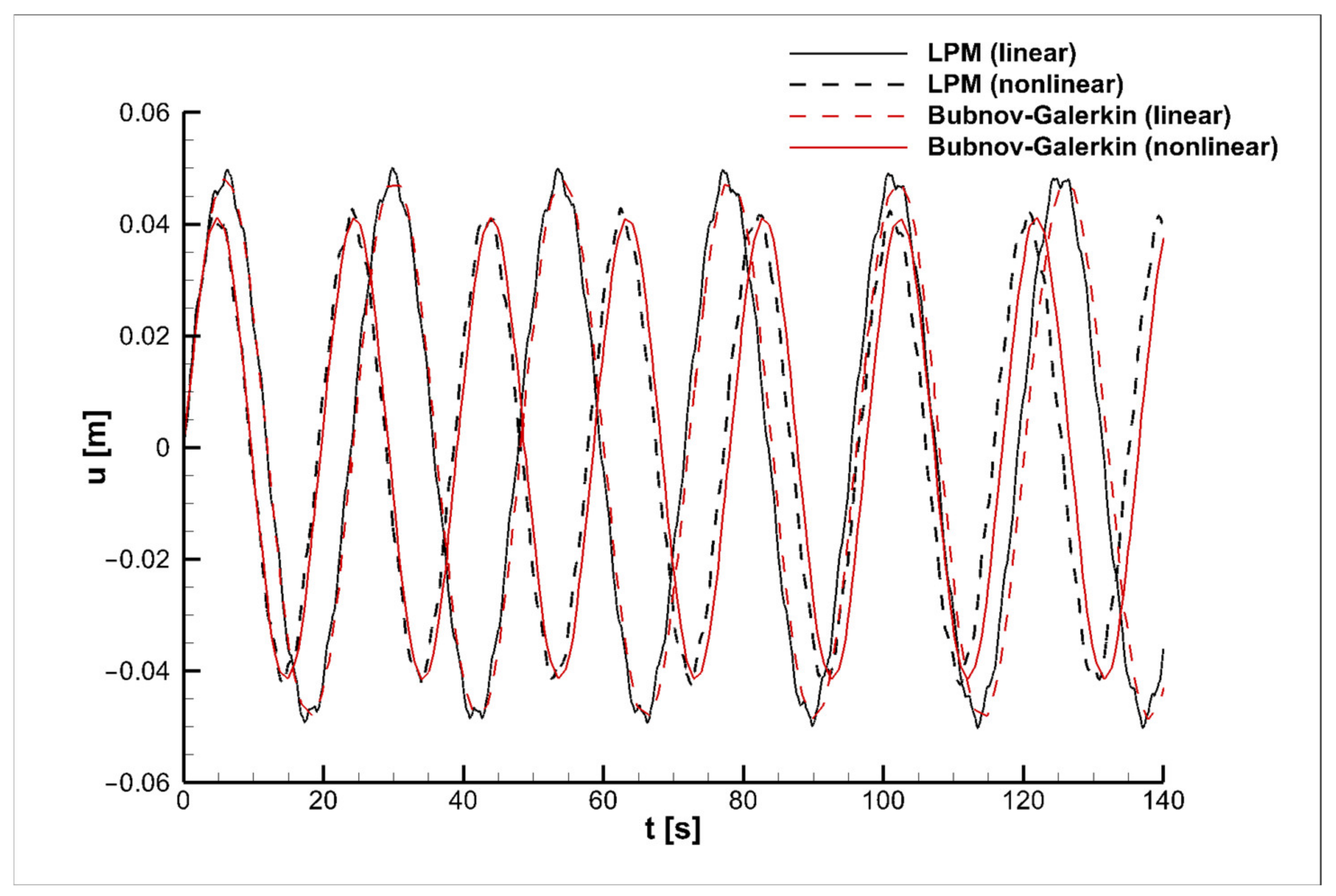
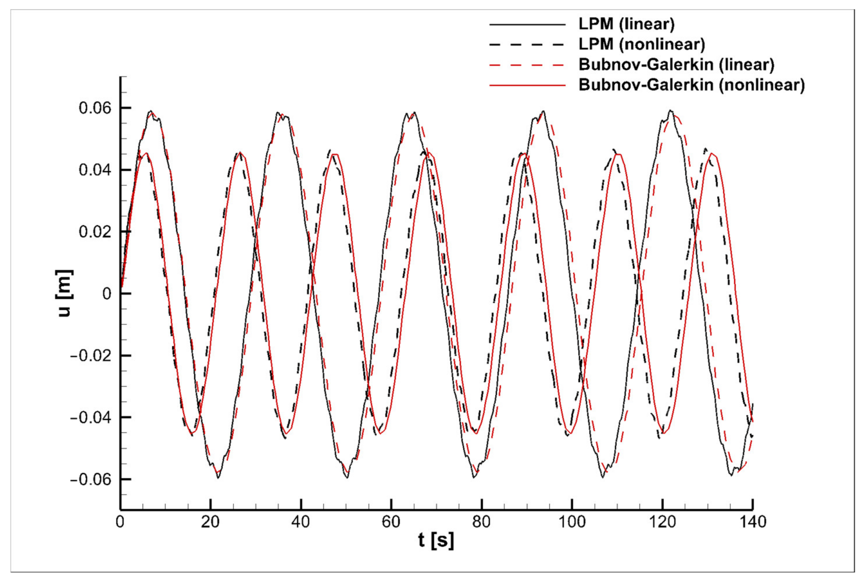
In Figure 2, Figure 3 and Figure 5, the thin solid black line shows the results for the linear model (b) and the dashed line those for the linear one (a) in the time interval $t=140\hspace{1em}\mathrm{s}$. The thick solid line represents the data on the nonlinear model (b) and the dash-dotted line the results for the nonlinear one (a). In Figure 4, the nonlinear models (a) and (b) coincide; therefore, the red solid line of (b) is chosen. Figure 2, Figure 3 and Figure 4 are constructed at $N=101,$ $\Delta t=5\times {10}^{-5}\mathrm{s}$, for the nonlinear model and $N=1001,$ $\Delta t={10}^{-5}\mathrm{s}$, for the linear one. 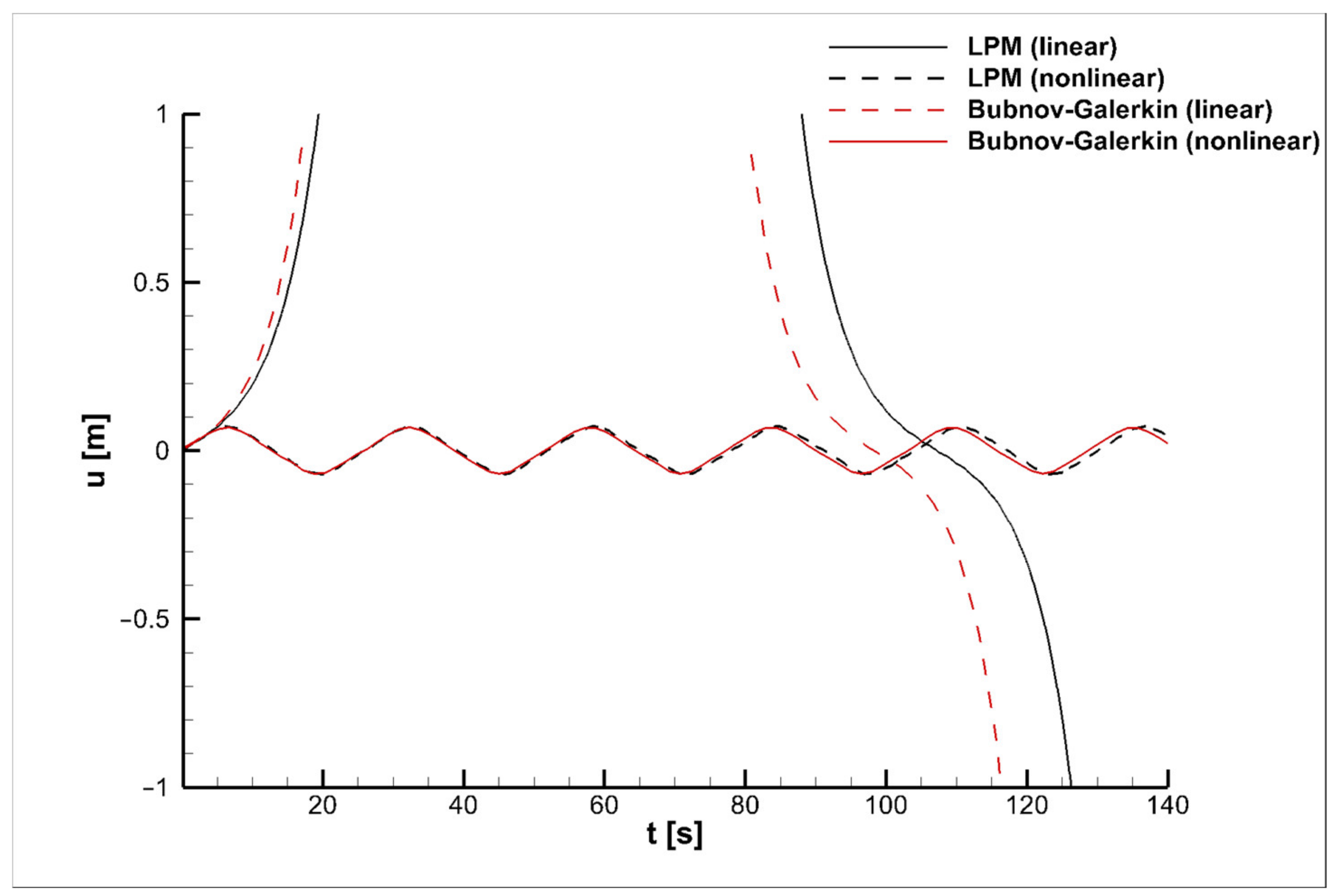In Figure 5, the parameters for both the models are $N=101,$ $\Delta t=5\times {10}^{-5}\mathrm{s}$.

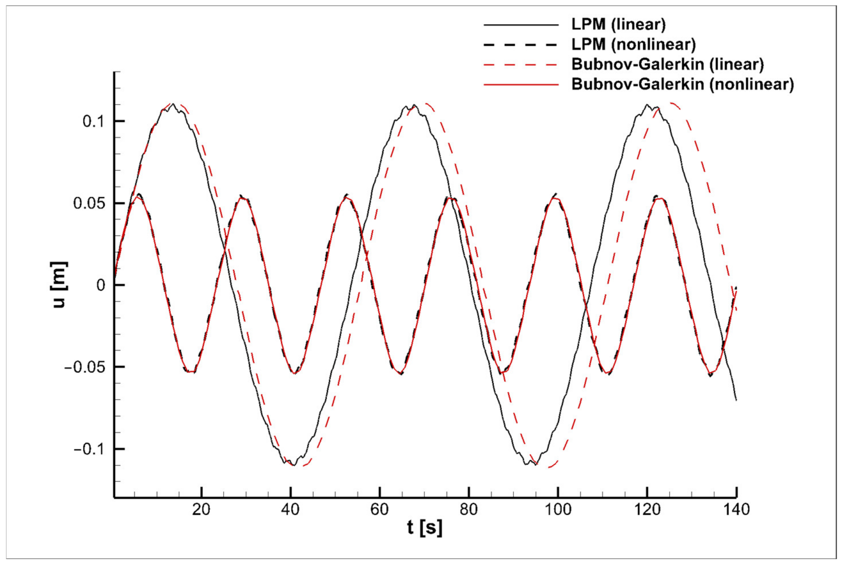
The graphs illustrate that the amplitude and period of the drill-string vibrations obtained by solving the nonlinear model are lower than those of its geometrically linear analogue for the considered values of angular speed $\Omega$. Noteworthy is that at the angular speeds of rotation $\Omega =0.083\hspace{0.17em}\mathrm{rad}/\mathrm{s}$ and $\Omega =0.167\hspace{0.17em}\mathrm{rad}/\mathrm{s}$, the amplitude of the nonlinear vibrations is slightly less than the amplitude for the linear case (Figure 2 and Figure 3), whereas the increase in the value of $\Omega$ results in the significant change in the vibration amplitude. At $\Omega =0.25\hspace{0.17em}\mathrm{rad}/\mathrm{s}$, the double increase in the geometrically linear vibration amplitude is observed (Figure 4). At $\Omega =0.33\hspace{0.17em}\mathrm{rad}/\mathrm{s}$, the drill-string vibrations calculated with the linear model rise sharply, while the nonlinear oscillatory process remains stable (Figure 5). It shows the importance of using nonlinear models for solving drilling problems, since they are more accurate and resistant to changes in parameters than linear ones.

Figure 2 and Figure 3 demonstrate the good consistency in the results of the current work (b) with sample data (a); namely, in the time interval up to 60 s, the solution curves almost coincide; then, over time, minor deviations can be distinguished. As can be seen from Figure 4, the differences in the results of (a) and (b) for the linear model are clearly distinguishable for lower values of angular speed when the same number of partitions in space is taken, while the results on the nonlinear model over the entire time interval coincide.

It is worth noting that for the convergence of the linear model, much more spatial partition points are required. As it is mentioned above, to calculate the nonlinear model in Figure 2, Figure 3 and Figure 4, the parameters $N=101,$ $\Delta t=5\times {10}^{-5}\mathrm{s}$ were taken, while for the linear model, the number of points was increased 10 times to $N=1001$, and the time step was chosen to be equal to $\Delta t={10}^{-5}\mathrm{s}$. In Figure 5, in view of the unlimited growth of the oscillation amplitude and the divergence of the linear model as a whole, the same parameter values were taken for both the models, namely, $N=101,$ $\Delta t=5\times {10}^{-5}\mathrm{s}.$ For this reason, the differences in the results of the linear model (a) and (b) are clearly noticeable. It also confirms the better convergence and greater stability of the nonlinear models compared with the linear ones, which require a smaller number of partition points in space when using the lumped-parameter method and, as a consequence, less time spent on the numerical implementation that plays an important role in the modeling process.

Thus, the good consistency of the obtained results with previously published data is demonstrated. It confirms the feasibility of using the lumped-parameter method in drilling problems for rod-element vibrations and justifies its further application for solving mathematical models of lateral vibrations in structures complicated by a variable equipment structure where there is no possibility to use well-known approaches.

5. Application of Parallel Programming

A small time step, the need to use a large number of partitions for the linear models and, as a result, a large number of iterations serve as the reasons for conducting the next stage of the study consisting in the optimization of the program code using parallel-programming tools.

The parallelization of the C++ code is here implemented using the Open Multi-Processing (OpenMP) library. The use of this library allows developing an algorithm working sequentially and in parallel, and it is one of the most popular parallel programming technologies used for shared memory computers [33]. Moreover, the OpenMP technology is quite effective to parallelize one-dimensional problems.

To analyze the advantages of using parallel programming, the spent time resources and the optimal number of threads, the program code was tested on linear model of lateral vibrations (23) with angular rotation speed $\Omega =0.167\hspace{0.17em}\mathrm{rad}/\mathrm{s}$ for various values of partition nodes and time step $\Delta t$ in the interval $t=60\hspace{1em}\mathrm{s}$.

The test results are shown in

Table 1. Program implementation time depending on the number of threads, iterations, partitions and the time step.

Number of Points	Iterations (mln)	Time Step (s)	Implementation Time Depending on the Number of Threads (s)
			1	2	3	4	5	6	7	8	9	10	11	12
11	0.6	0.0001	8.6	6.6	8.2	9.2	14.3	18.5	20.7	21.3	23.3	27.4	29.3	30
31	0.6	0.0001	28.2	17.5	16.9	19.3	23.9	25.8	27.2	27.9	31.4	35.2	36	36.4
51	0.6	0.0001	47.6	28	22.5	23.2	34.1	32.9	33.4	33.1	38	40.9	42.2	42.8
101	1.2	0.00005	205.3	109.5	81.5	75.9	103.7	98.8	97.1	92.8	109.6	108.9	109.4	110.4
201	1.2	0.00005	388.1	215.3	158	140.9	190.5	176.3	172.6	150.9	189.2	187	191.8	184.9
401	1.2	0.00005	814.7	424.7	314.8	267.8	372.5	316	292.1	262.7	326.8	312.5	301.1	286.3

. The table rows include the nodes, the number of iterations, the time step and the code-implementation time depending on the number of threads used. The computation time for one thread is highlighted in red, i.e., the implementation of the program without parallelization. The cells containing the shortest implementation time are highlighted in yellow. As can be seen from the table, the use of a large number of computation threads gives much worse results than those without parallelization for 11 partition points, which is understandable for arrays with a small number of elements (11–31). However, when the number of partition points equals or exceeds 51, the use of a large number of threads up to 12 gives a considerable time gain compared with using one thread. It can also be seen that the utilization of two threads is quite optimal for the minimum number of partition points (11). When we split the rod into 31 and 51 parts, the optimal number of threads is 3; for more than one hundred partition points, the optimal number of threads is 4 in accordance with the spent implementation time.

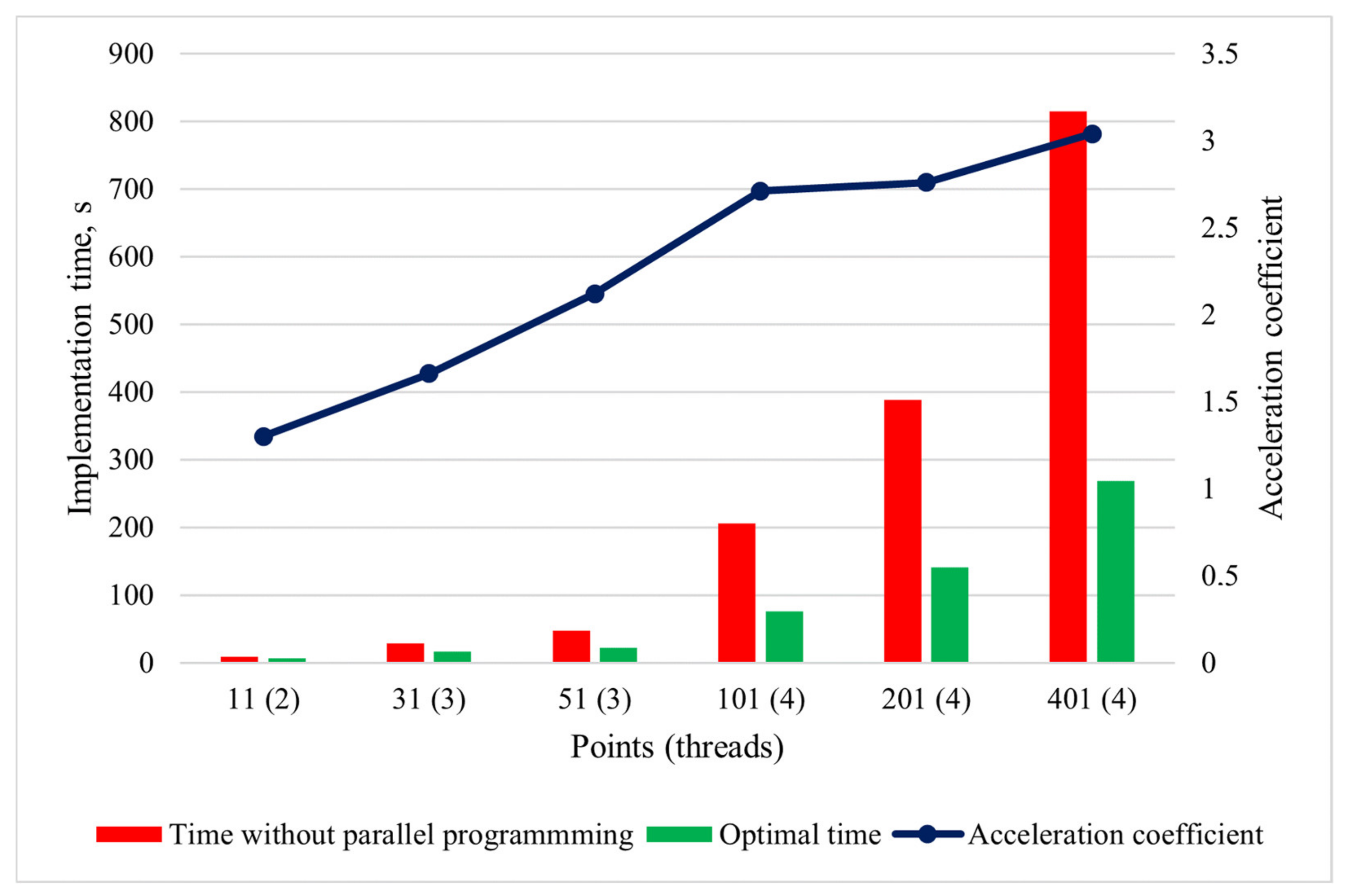
The justification of the use of parallel programming is also analyzed. The estimation of the acceleration coefficient of the code implementation time is performed when the optimal number of threads is utilized (

Table 2. Analysis of the code implementation time using parallel-programming tools.

Number of Points	Implementation Time for 1 Thread (s)	Optimal Time (s)	Optimal Number of Threads	Acceleration Coefficient
11	8.6	6.6	2	1.3
31	28.2	16.9	3	1.66
51	47.6	22.5	3	2.12
101	205.3	75.9	4	2.71
201	388.1	140.9	4	2.76
401	814.7	267.8	4	3.04

).

Table 2 shows the values of the program acceleration coefficient using the OpenMP library for the different number of partition points and demonstrates the advantages of using parallel programming. When the low number of points (11) is used, the program implementation time decreases by 1.3 times; then, when increasing the number of partitions to 401, we can observe a more-than-threefold decrease in the computation time, namely, the time needed for program completion reduces from 13.6 to 4.5 min. It clearly demonstrates the importance of using parallel programming when solving the considered nonlinear model of the drill-string lateral vibrations. The acceleration coefficient depending on the different number of partition points is shown in Figure 6.

6. Analysis of System Discrete Partitioning

The next stage of the research study is to study how the accuracy of the obtained results depends on the number of partition points. When the number of points increases, the computation accuracy logically rises; however, the program implementation time also grows. This raises the question on the justification of the used computational costs and necessitates the analysis on the optimal number of the drill-string partitions from the “implementation time—computational accuracy” viewpoint.

To estimate the computation error, the results of [19] for the plane case are taken. The accuracy is estimated by comparing the sample data with the obtained results. For algebraic verification, the WPF Application developed by the authors of the current work in the C# language is utilized. The window application compares the loaded file data at the closest time points and calculates the computation error (maximum error and standard deviation). The results of the drill-string lateral displacements for angular speed of rotation $\Omega =0.167\hspace{0.17em}\mathrm{rad}/\mathrm{s}$ are taken as comparative data.

Table 3. Error estimation for the linear model of the drill-string vibrations at $\Omega =0.167\hspace{0.17em}\mathrm{rad}/\mathrm{s}$.

Number of Points	Max Error (mm)	Standard Deviation (mm)	Implementation Time (s)
11	90.37	42.28	137.63
51	55.29	27.00	595.95
101	31.86	16.11	1089.97
201	20.71	9.89	1948.62
301	16.51	7.73	3027.72
401	14.31	6.66	3087.12
501	12.78	6.02	3763.93
601	11.68	5.58	4564.72
701	11.21	5.27	5284.03
801	10.87	5.04	7820.47
901	10.59	4.86	8594.73
1001	10.37	4.72	9233.07

shows the results of comparing the obtained data of the linear model with the results for the plane case of [19]. The table includes the computation time and error indicators (standard deviation and maximum error) depending on the number of nodes. It is shown that the error is quite high when the minimum number of partitions (11) is considered; however, as the number of points rises, the values of both error indicators decrease, and the implementation time increases. It is worth noting that due to the use of parallel programming, the time spent on the code implementation significantly reduces, which allows the data to be computed and tested with a large number of partitions and a sufficiently small time step.

.

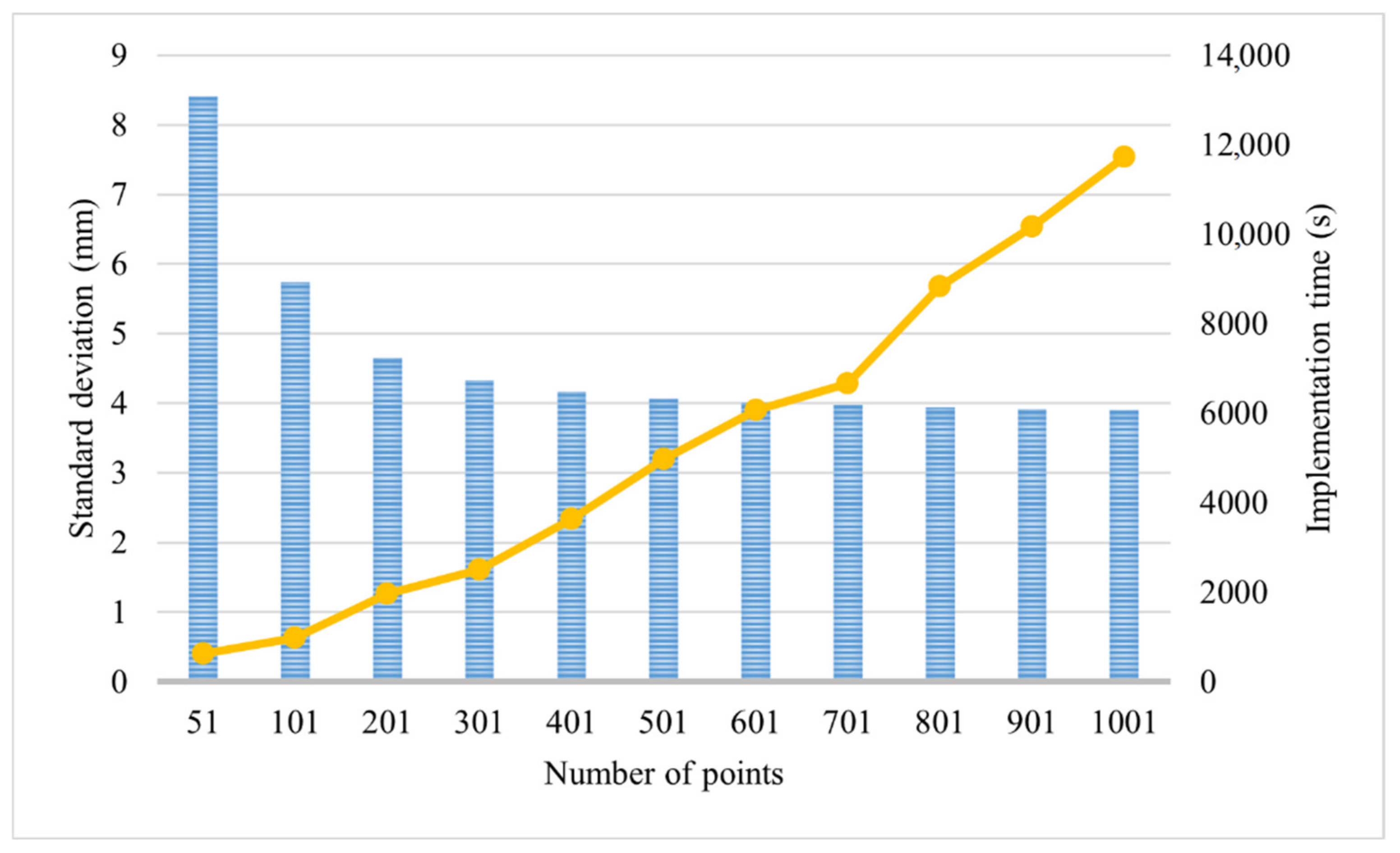
As can be seen from Table 3, for the number of partitions equal to 51, the maximum error and standard deviation decreased by 1.6 times compared with the case with 11 partitions with the same number of iterations, while the time spent on computation increased by 4.3 times (from 2.3 to 9.9 min). When 101 points are considered, the maximum error decreases by 2.83 times, and the standard deviation by 2.62 times, and the computation time increases to 18 min compared with the case with 11 points with the same time step. For a large number of partitions, we can observe minor changes in the error indicators. The standard deviation at 1001 points changes by 3 mm and 1.3 mm compared with the cases with 301 and 501 points and the maximum error by 6.1 mm and 2.4 mm, respectively, while the implementation time increases by 3 and 2.45 times. Starting from the value of 401 partitions, the change in the standard deviation does not exceed 0.63 mm. It follows that using a large number of partition points is impractical from the point of view of “implementation time—computational accuracy”.

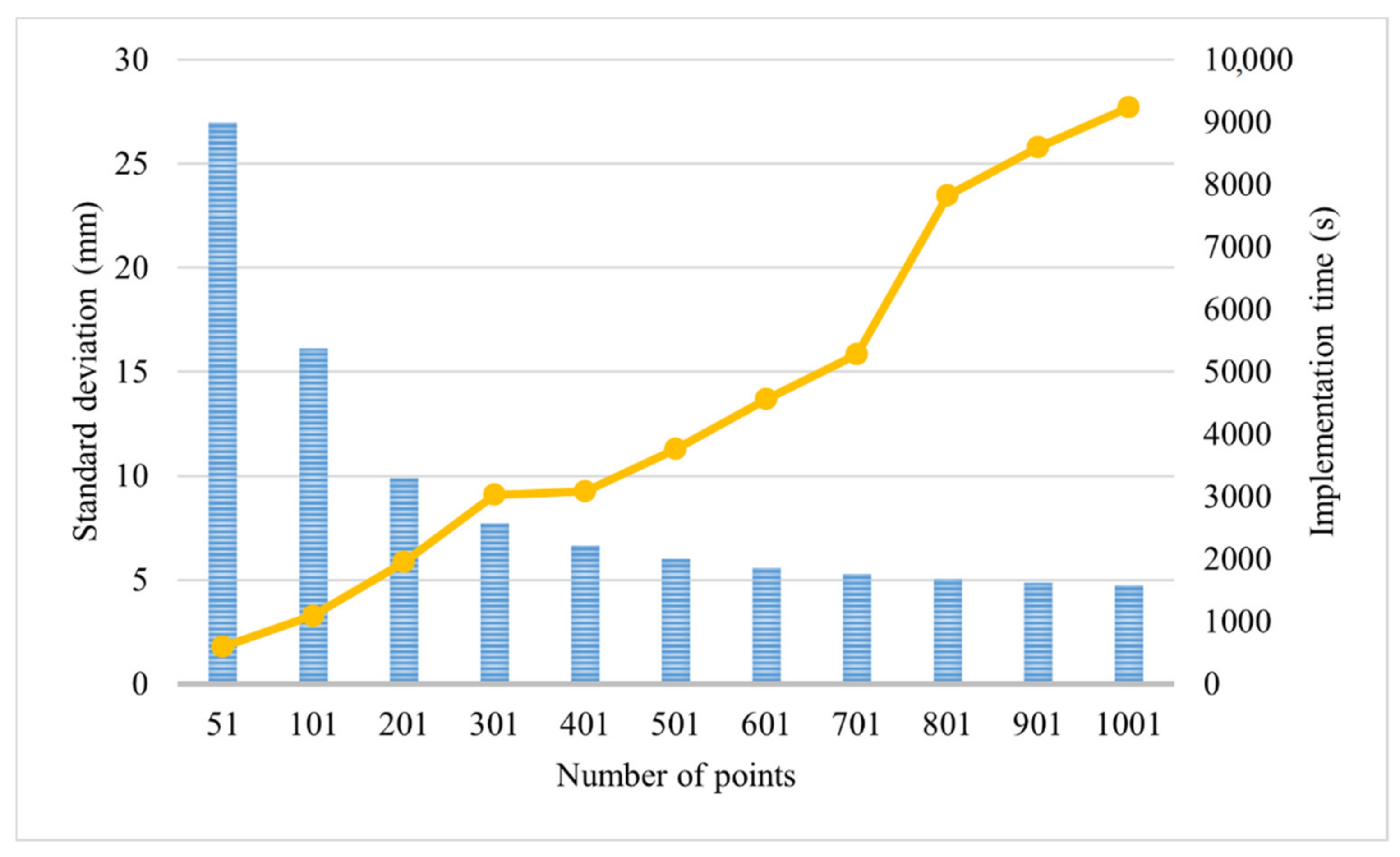
Figure 7 and Figure 8 demonstrate the dependence of the error indicators on the number of partition points for the linear and nonlinear models. The bar graph reflects the standard deviation, and the point curve shows the program implementation time. According to the constructed graphs, the optimal number of partition points from the point of view of “implementation time—computational accuracy” is 300–400, whereas numbers of partitions over 700 can be ignored, since they only give a slight improvement of the error indicators and, at the same time, a significant increase in the implementation time.

A better convergence of the nonlinear model than that of the linear one requires the estimation of the nonlinear-model computation error. The error indicators of the nonlinear model depending on the number of nodes are shown in

Table 4. Error estimation for the nonlinear model of the drill-string vibrations at $\Omega =0.167\hspace{0.17em}\mathrm{rad}/\mathrm{s}$.

Number of Points	Max Error (mm)	Standard Deviation (mm)	Implementation Time (s)
11	76.99	36.06	150.40
51	16.07	8.41	632.07
101	10.07	5.73	971.52
201	8.67	4.65	1958.70
301	7.95	4.32	2499.00
401	7.43	4.16	3638.00
501	7.35	4.06	4964.20
601	7.30	4.01	6064.00
701	7.26	3.97	6650.70
801	7.23	3.94	8825.60
901	7.21	3.91	10,165.00
1001	7.20	3.89	11,729.00

. The trend presented in Table 3 does not change. With an increase in the number of partitions, the error indicators decrease, and the implementation time increases; however, starting from a particular number of points (201–301), the improvement of the error indicators is not equivalent to the increase in the implementation time, which implies the use of a large number of nodes to be impractical. The optimal number of partitions for the nonlinear model is considered to equal 201 from the “implementation time—error indicators” viewpoint, which is two times lower than the optimal number of partitions needed for its linear analogue. It also confirms the better convergence of the nonlinear model compared with the linear one.

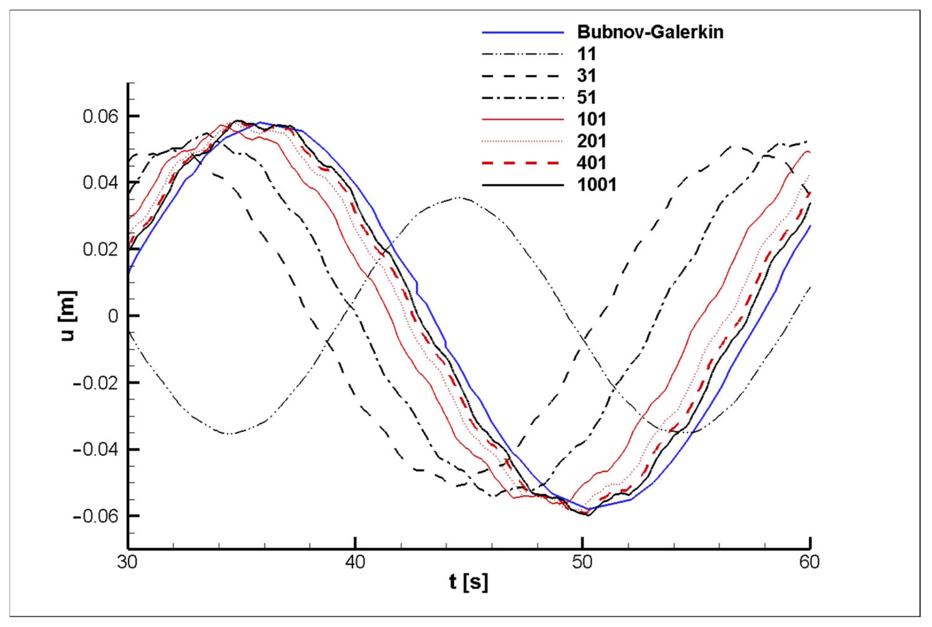
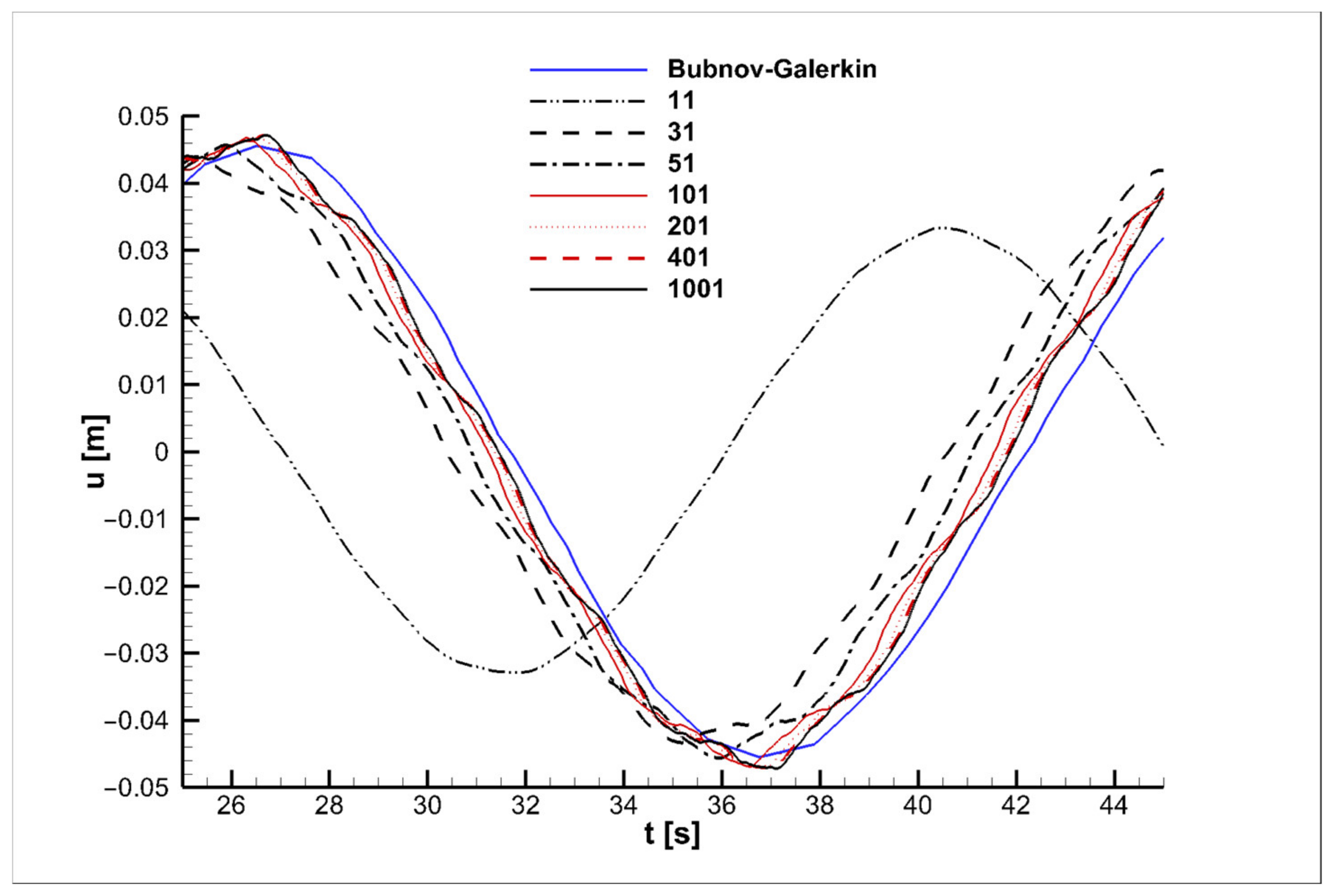
The convergence of the obtained curves for the drill-string lateral displacements with the sample data depending on the number of partition points is shown in Figure 9 for the linear model and in Figure 10 for the nonlinear one. Different types and colors of curves correspond to the results for the different numbers of points. As the graphs show, the increase in the number of the drill string partition points results in a higher convergence of the research results to the sample data obtained using the Bubnov–Galerkin method. Moreover, the use of the LPM allows not only more accurate estimating the overall picture of the drill string oscillatory process without using additional approximation functions, but also studying each segment of the drill string in detail.

7. Conclusions

In this paper, the effectiveness of the lumped-parameter method (LPM) in solving nonlinear problems of drill-string vibrations is studied. A good consistency of the results of the test problem related to the longitudinal vibrations of a horizontal drill string with a static compressive load at the end with the results of other authors is obtained. The discretization of the nonlinear model of the lateral vibrations of a vertical rotating drill string in a supersonic gas flow using the LPM shows the better convergence and stability of the solution of the nonlinear model compared with its linear analogue. Moreover, the comparative analysis of the results with those obtained using the Bubnov-Galerkin method demonstrates the great consistency between them when increasing the number of the drill string partition points.

The conducted analysis of the optimal number of drill-string partitions reveals that in the case of the nonlinear model, the number of partitions of 200 is quite sufficient from the “implementation time—computational accuracy” viewpoint and is almost two times less than the preferable number of partition points needed for obtaining adequate results using the linear model (300–400 points).

The developed program for solving the discrete models allows the solution to the problems to be found with various numbers of partition points and affecting loads. It gives the possibility to use the constructed algorithm when solving more complex problems with heterogeneous structures of the research object. The performed optimization of the numerical algorithm using parallel programming indicates the effectiveness of its application due to the great number of partitions that leads to the increase in the solution accuracy.

The research results also show that LPM may be further effectively utilized for studying the dynamics of nonlinear systems with variable structure when there is no possibility to use other mathematical approaches.