Analyzing the Effect of Filtering and Feature-Extraction Techniques in a Machine Learning Model for Identification of Infectious Disease Using Radiography Imaging

Abstract

The massive adaptation of reverse transcriptase-polymerase chain reaction (RT-PCR) has facilitated efforts to battle against the COVID-19 pandemic that has inflicted millions of individuals around the world. Besides RT-PCR, radiography imaging examinations yields valuable insight for detecting and diagnosing this infectious disease. Thus, this paper proposed a computer vision and artificial-intelligence-based hybrid approach aid in efficient detection and control of COVID-19 disease. The study utilized chest X-ray images to segregate COVID-19 positive cases among healthy individuals by exploiting several combinational structures of image filtering, feature-extraction techniques, and machine learning algorithms. It analyzed the effects of three noise removal filters and two feature-extraction techniques on performance of several machine learning and deep-learning-based classifiers. The proposed schemes first remove unnecessary noise using a conservative smoothing filter, Crimmins speckle removal, and Gaussian filter. It then employs linear discriminant analysis (LDA) as linear method and principal component analysis (PCA) as non-linear feature-extraction technique to extract highly discriminant feature sets. Finally, it uses these feature sets to train various classification models, including convolutional neural network (CNN), support vector machine (SVM), and logistic regression (LG). Evidently, the proposed conservative smoothing filter with single peak to maintain symmetry in horizontal and vertical directions for enhancement of image, along with LDA and SVM, secured an overall classification accuracy of 99.93%. Experimental results show that, besides achieving high accuracies, the incorporation of feature-extraction techniques significantly reduces the computational time of the proposed model.

1. Introduction

COVID-19 is linked to a number of other dangerous diseases, and the most common symptoms, such as fever and cough, make proper diagnosis difficult for health care providers. Thus, COVID-19 has had a disastrous effect on the global population since its entrance into the human population in late 2019, with the number of infected persons continuously rising [1]. With the lack of widely available medicines and the persistent strain on many healthcare systems throughout the world, rapid screening of suspected COVID-19 patients and subsequent isolation is critical to preventing the virus from spreading further. The current gold standard for patient screening and accurate diagnostic is reverse transcriptase-polymerase chain reaction (RT-PCR), which uses respiratory samples to infer the presence of COVID-19. Even though RT-PCR is regarded as the most reliable screening test, it often takes a couple of days, especially in regions such as remote areas of Pakistan, while rapid preventive procedures and clinical care are required in the meantime. However, the usage of recent rapid diagnostic tests, which are susceptible to such precise issues, has increased, thus potentially limiting health resources [2].

Despite RT-PCR success, it is a time-consuming manual technique with long turnaround times, with results arriving up to several days after the test. Moreover, because of inadequate standardized reporting, its inconsistent sensitivity, and wide range of total positive rates, alternate screening approaches are required [3]. COVID-19 can be diagnosed quickly and efficiently with effective screening, which can save healthcare systems’ money. Prediction approaches that include numerous functions to estimate infection risks have been developed with the goal of assisting medics globally in patient triage, particularly in light of limited health resources. These models exploit laboratory testing, clinical symptoms, X-rays, computed tomography (CT) scans, and integration as potential features for prediction and classification of COVID-19 patients.

Moreover, X-ray and CT imaging has been widely utilized as a powerful alternative tool due to rapid evaluation in emergency cases. Furthermore, X-ray imaging provides specific advantages over the other imaging methods evaluated in terms of availability, accessibility, and rapid testing [4]. Moreover, the availability of portable X-ray imaging technologies eliminates the need for patient transportation or physical contact between healthcare workers and suspected infected patients, allowing safer testing and more effective virus isolation. Despite its evident benefits, radiography examination has a major challenge: a scarcity of experienced professionals who can perform the analysis at a time when the number of potential patients continues to climb. Still, chest X-ray and CT scans yield promising results, as they are usually analyzed by radiologists who are experts in their field. However, many patients visit radiologists every day, and the diagnosis process takes so long that disparities can quickly mount, necessitating the use of computer-assisted diagnostic (CAD) to reduce false negatives while also saving time and money. Furthermore, automated artificial-intelligence-based (AI) CAD methods are thought to perform particularly well in the diagnosis of pulmonary illness [5]. As a result, a smart, automated system capable of effectively analyzing and interpreting radiography imaging can certainly reduce the pressure on professional radiologists while also consolidating victim care [1].

Thus far, several effective COVID-19 vaccines have been developed by well-known businesses all over the world. However, following regulatory rules for safety precautions, wearing masks, and social distancing remain the three most effective COVID-19-prevention strategies [6]. AI-based applications, on the other hand, are a useful technique to assist physicians in dealing with coronavirus and improving medical care. Machine learning and deep learning techniques are commonly employed to detect disease patients, while mathematical modeling and social network analysis (SNA) approaches are utilized to forecast the pattern of disease outbreaks [1]. For instance, authors in [7] identified COVID-19 affected patients in five-class (healthy, lung opacity, bacterial pneumonia, viral pneumonia, and COVID-19) and three-class (healthy, pneumonia, and COVID-19) classification problems by creating two databases. It investigated three pre-trained networks (DenseNet161, ResNet50, and InceptionV3) and finally suggested a convolutional neural network (CNN)-based ensemble scheme to secure an overall 98.1% accuracy in the five-class scenario and 100% accuracy in the three-class scenario. Similarly, researchers in [8] exploited DenseNet201 instead of DenseNet161 to propose another weighted-average-based ensemble network by investigating X-ray images to identify COVID-19-positive patients among healthy. Their developed system attained an accuracy of 91.62%. In another study, authors [9] proposed deep-learning-based network capable of identifying COVID-19-affected individuals from chest X-ray images in healthy and/or pneumonia patients. The suggested technique fuses two modified, pre-trained models (on ImageNet), namely MobileNetV2 and VGG16, sans their classifier layers and achieves improved classification accuracy (96.48% for the three-class classification problem) on the two currently publicly available datasets using the confidence fusion method.

Besides this, researchers have devised a number of feature-extraction techniques along with machine learning algorithms to minimize the dimension of data, lowering computational and spatial expenses dramatically to diagnose COVID-19-affected or pneumonia patients. For example, authors in [10] used CNN to obtain features and then incorporated SVM to improve classification performance using five-fold cross-validation on a COVID-19 dataset that they had collected. Using a well-trained model, the influence of COVID-19 on persons with pneumonia and pulmonary disorders on the dataset gathered in chest radiography images was determined. They secured specificity of 96% and sensitivity of 90%. To diagnose pneumonia in low-resource and community settings, researchers in [11] used SVM, logistic regression (LG), and decision trees (DT) classifiers. The researchers used a feature-selection technique to identify six critical traits and then used dataset instances to train the learning models. The DT model, which had an area under the curve (AUC) of 93 percent, performed better than the other models during the testing phase. In addition to these, computer scientists exploited automated feature-extraction techniques; for example, individuals in [12] segregated COVID-19-positive patients and healthy persons by proposing CNN and LG models. Moreover, they extracted the relevant features using principal component analysis (PCA) to achieve a performance accuracy of 100%. Likewise, researchers in [13] analyzed the performance of transfer-learning-based deep-learning model. It extracted relevant representatives from radiography images using VGG16 followed by PCA to further reduce the extracted number of features. Later, they trained four different classifiers (SVM, deep-CNN, extreme learning machine (ELM), and online sequential-ELM) and concluded that bagging ensemble with SVM bypassed other models by securing 95.7% accuracy.

Although machine learning techniques showed promising results in devising diagnostic systems, scientists have suggested several intelligent diagnostic tools based on computer vision (CV) techniques by analyzing various image-filtering schemes, for instance [14]. Similarly, authors in [15] used a threshold filter to remove the lungs region, then upgraded the images with Otsu thresholding and harmony search optimization (HSO) to evaluate COVID-19 disease severity using CT images. A detailed review of potential AI-based futuristic approaches for identifying and detecting COIVD-19 infectious disease can be found in [1].

The approaches for diagnosing the result of COVID-19 cases that were previously provided have several flaws. First, most of the models are trained over limited data without cross-validation and thus may result in under-fitting and over-fitting. Second, they do not provide any information regarding the efficiency of the model in terms of time. Moreover, very limited work has been published that incorporated CV techniques, especially image-filtering along with machine learning classifiers. The objective of this study is to improve the classification performance metrics and investigate the essential features that impact the performance outcome of proposed model. As a result, the study’s major goal is to improve medical decision making in order to lower COVID-19 mortality. To do this, the study proposed a hybrid scheme by incorporating CV techniques along with advanced machine learning and deep learning classifiers to segregate the COVID-19 cases from normal patients. It assists clinicians in providing proper medical care to patients who are at high risk. The key objectives include:

• Propose smoothing filters with single peak to maintain symmetry in horizontal and vertical directions for enhancement of images;
• Examine the effect of several filtering techniques (conservative smoothing, Crimmins speckle removal, and Gaussian filters) in diagnosing COVID-19;
• Exploit a supervised linear feature-extraction technique (linear discriminant analysis (LDA)) as well as unsupervised non-linear feature-extraction technique (kernel PCA);
• Investigate and analyze the significance of employing linear and non-linear feature-extraction techniques with linear and non-linear machine learning classifiers;
• Design various combinational scheme of filters and feature-extraction techniques to demonstrate its impact on the diagnostic performance of an AI-based system;
• Examine the performance and provide comparative analyses of each combinational scheme in terms of time;
• Present a simple but highly accurate deep-learning-based model that can be used with other conventional clinical COVID-19 testing to remove false-alarm probability;
• Provide analysis to indicate that the proposed scheme outperformed prior studies by securing 100% accuracy while segregating COVID-19-positive cases among normal ones in a minimal amount of time.

The rest of this script starts with description of dataset and methods exploited, then moves on to a quick review of experimental setup and detailed presentation of results obtained with critical discussion and compares the performance with prior studies. Finally, it presents concluding remarks.

2. Dataset Description and Methods

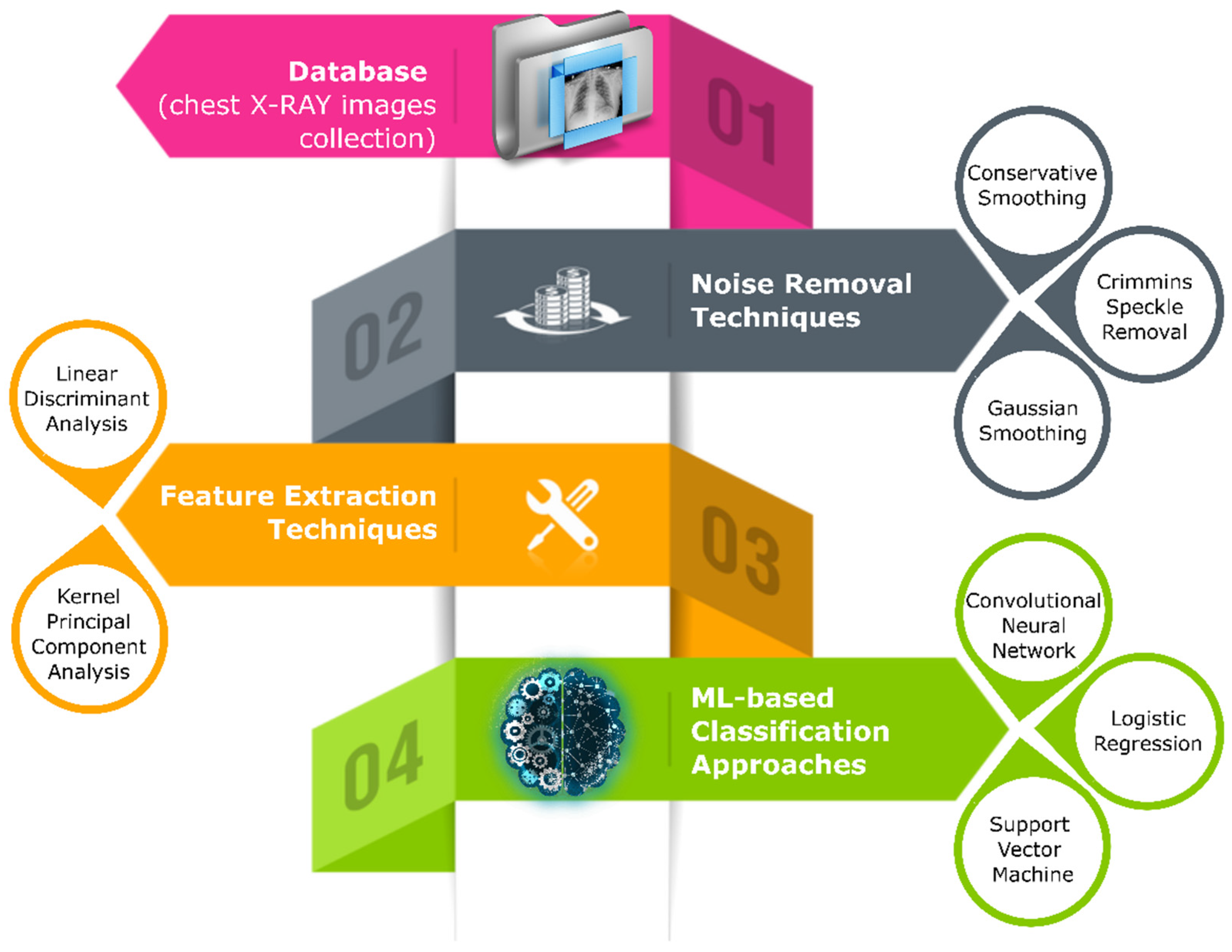
The study proposes a hybrid scheme by combing machine learning models with CV techniques as depicted in Figure 1. The study acquired the X-ray image instances of healthy and COVID-19-affected patients from various online sources and later fed them to three distinct image-filtering techniques (conservative smoothing filter, Crimmins speckle removal filter, and Gaussian smoothing filter) separately to generate three new datasets by eradicating unwanted noise from radiography images. Next, two feature-extraction techniques (LDA and PCA) took each filtered dataset instance to extract the most relevant features. Finally, machine learning classifiers (CNN, LG, and SVM) used extracted imported features for training and testing purposes to segregate COVID-19-positive cases from normal/healthy (COVID-19-negative) patients.

This study acquired chest X-ray images of normal, healthy individuals and COVID-19-affected patients from various publicly available online sources for training multiple machine learning classifiers and to analyze the effect of the image filtering and feature-extraction technique. The sources include: COVID-19 Radiography Database (CRD) [16] and Actualmed COVID-19 Chest X-ray Dataset Initiative (ACCDI) [17]. During the course of this experimental work, the dataset [16] contained 33,920 chest X-ray images, out of which 3616 images belonged to COVID-19-positive confirmed cases. Thus, this study accumulated 58 images of confirmed COVID-19-positive cases and 127 X-ray images of normal individuals from ACCDI and 3616 COVID-19+ X-ray images and 3547 X-ray images of normal patients from CRD, as outlined in

Table 1. Dataset information.

Dataset	Case-Type/Class		Total
	COVID-19	Normal
CRD	3616	3547	7163 (97.48%)
ACCDI	58	127	185 (2.52%)
Total	3674 (50%)	3674 (50%)	7348 (100%)

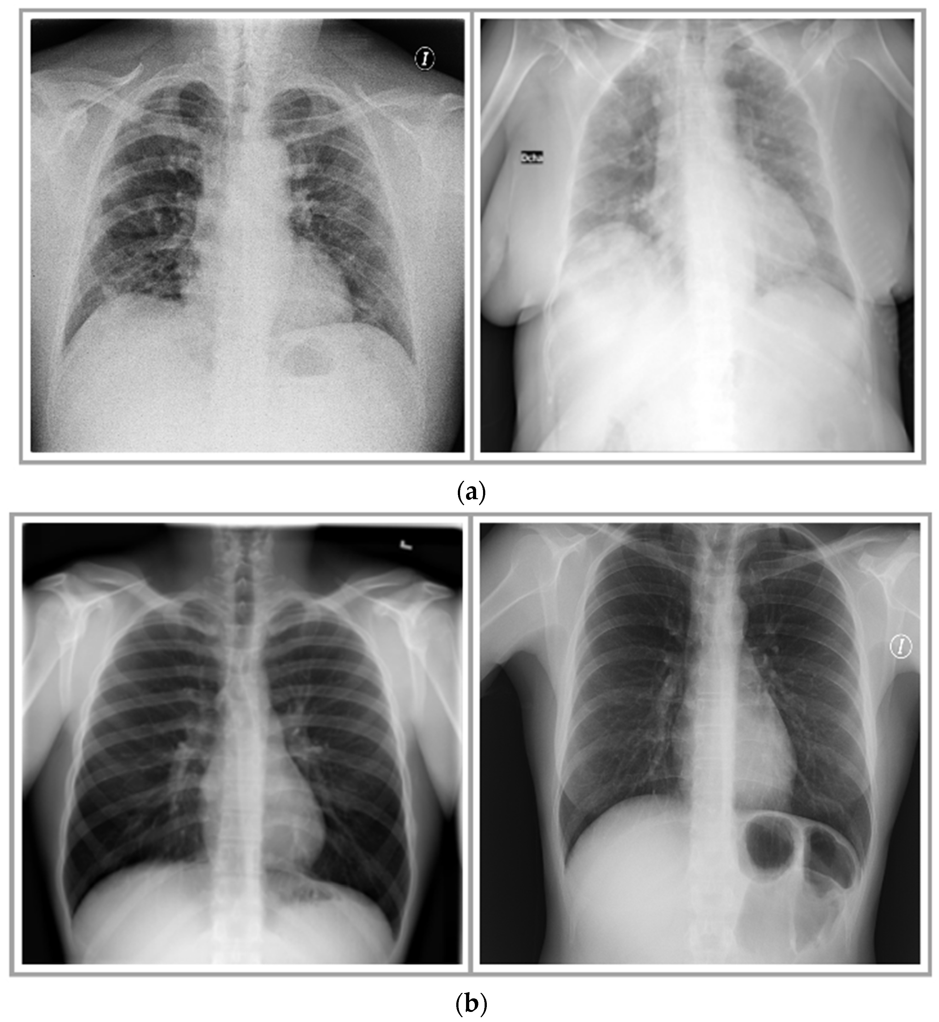
. The radiography images taken from the dataset [16] are uniform in size (height × width: 256 × 256); however, the images present in [17] vary in size; thus, before proceeding further, this study resized these images to a fixed size (height × width: 256 × 256). Figure 2 shows few instances of X-ray images of COVID-19 cases and healthy individuals. A division of 20–80% was made in the compiled dataset as test and train sets, respectively. Moreover, 20% of the training data was further used for validation to avoid overfitting and underfitting issues.

2.1. Image Noise Removal Techniques

When an imaging system captures an image, the vision system meant for it is frequently unable to use it directly. The variations in illumination, random fluctuations in intensity, or inadequate contrast may distort the image, which must be dealt with in the early phases of vision processing. Typically, image noise can be categorized into three main categories: photoelectronic, impulse, and structured. Photoelectronic further includes Gaussian noise and Poisson noise. Gaussian noise occurs due to the discrete nature of radiation of warm items, while Poisson exists due to the statistical nature of electromagnetic waves (gamma- or X-rays). The impulse noises include pepper noise, salt noise, and salt and pepper noise; these mostly occur due to sudden disturbance in the image signal. On the other hand, speckle noise occurs during image acquisition.

Such noises hinder the classification performance of machine learning classifiers. Naturally, the initial step should be to lessen the noise’s influence before moving on to the next stage of processing. Various image pre-processing techniques have been developed to achieve this goal, including image filtering (such as mean, median, Laplacian, Gaussian, conservative, and frequency filter), which lowers noise while enhancing useful information such as edges in images. Several approaches (conservative smoothing filter, Crimmins speckle removal filter, and Gaussian filter) for image enhancement discussed in this section are exploited to remove these unnecessary characteristics. A compact introduction of each filter is presented below.

2.1.1. Conservative Smoothing Filter

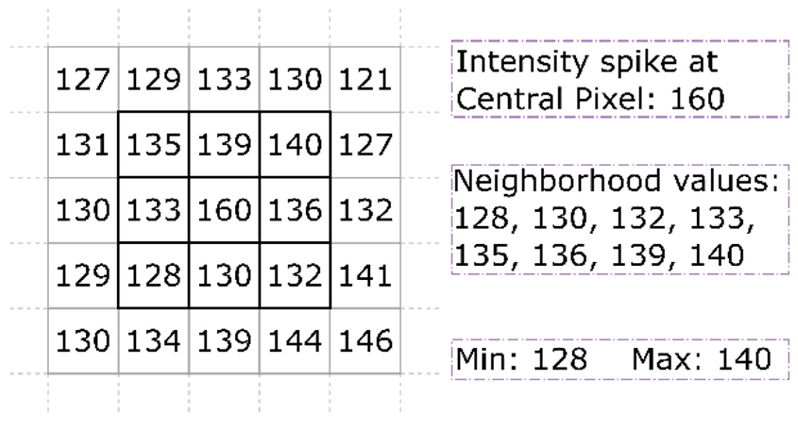
Conservative smoothing is a widely adopted noise removal filter specifically designed to eliminate salt and pepper noise. It uses the most basic and fast filtering algorithm that trades noise suppression strength for preserving high spatial frequency detail. It attenuates noise by performing local operations to fix the intensity of each pixel roughly commensurate with its surrounding pixels. Contrary to the median filter that achieves this through non-linear rank-selection procedure, conservative smoothing simply bounds the intensity of pixel of interest within the intensities range determined by its surrounding neighbors. This is done using a process that initially determines the maximal and minimal values of pixels surrounding the pixel of interest present within the window in question, as shown in Figure 3. It checks the intensity of the pixel at question; if it falls within determined range, then the pixel remains unaffected in the output image. However, if the pixel intensity value falls shorter than minimal value, its value is set to minimal value of the determined range. On the other hand, if the intensity of the pixel in question is greater than the maximal value, its value is set to maximal value.

As illustrated in Figure 3, the filtering conservatively smoothes the local pixel neighborhood. The pixel under consideration within the windowed region has an intensity spike with intensity value of 160, whereas its eight neighboring pixels have 128, 130, 132, 133, 135, 136, 139, and 140 values. The conservative smoothing determined 140 as the maximal value and 128 as minimal value. Hence, the intensity of the central pixel is greater than the maximal value. In such scenario, the filter replaces the central pixel intensity value with maximal value. Thus, unlike mean and median filters, conservative smoothing filtering has a more subtle effect and less corrupting at the image edges. However, it is less successful at eliminating additive noise such as Gaussian noise.

2.1.2. Crimmins Speckle Removal Filter

Similar to the conservative smoothing filter, this filter is explicitly formulated to minimize image speckle noise via the Crimmins complementary hulling algorithm by comparing the intensity of each pixel with the eight nearest neighboring pixels in an image [18]. It reduces the speckle index of that image by adjusting the values of pixel to make it more representative of its surroundings. It either increments or decrements the intensity value of central pixel based on the relative values of pixels within the eight-neighborhood window. As shown in Algorithm 1, the image is first fed to the pepper filter that determines if value of the pixel under examination (window’s center or current pixel) is darker than its northern neighbor; if so, the current pixel value is incremented twice. In other words, the current pixel is lightened. Next, it is again passed through the pepper filter to examine with the southern pixel, and intensity is incremented if it is darker than its southern neighboring pixel. The image is then fed to the salt filter, where the condition “lighter than” is checked with the northern neighbor, and if condition proves true, the intensity of the current pixel is decremented. The sequence is repeated with another salt filter for comparison with the southern neighboring pixels.

Algorithm 1: Pseudo code for working of Crimmins speckle removal
01	//suppose x, y, and z as three consecutive pixels (north-south direction) under examination
02	For each iteration
03	Pepper filter //adjust dark pixels
04	For all four directions
05	If x ≥ y + 2, then y = y + 1
06	If x > y & y ≤ z, then y = y + 1
07	If z > y & y ≤ x, then y = y + 1
08	If z ≥ y + 2 then y = y + 1
09	Salt filter //adjust light pixels
10	For all four directions
11	If x ≤ y − 2, then y = y − 1
12	If x < y & y ≥ z, then y = y − 1
13	If z < y & y ≥ x, then y = y − 1
14	If z ≤ y − 2, then y = y − 1
15	end for loop

2.1.3. Gaussian Smoothing Filter

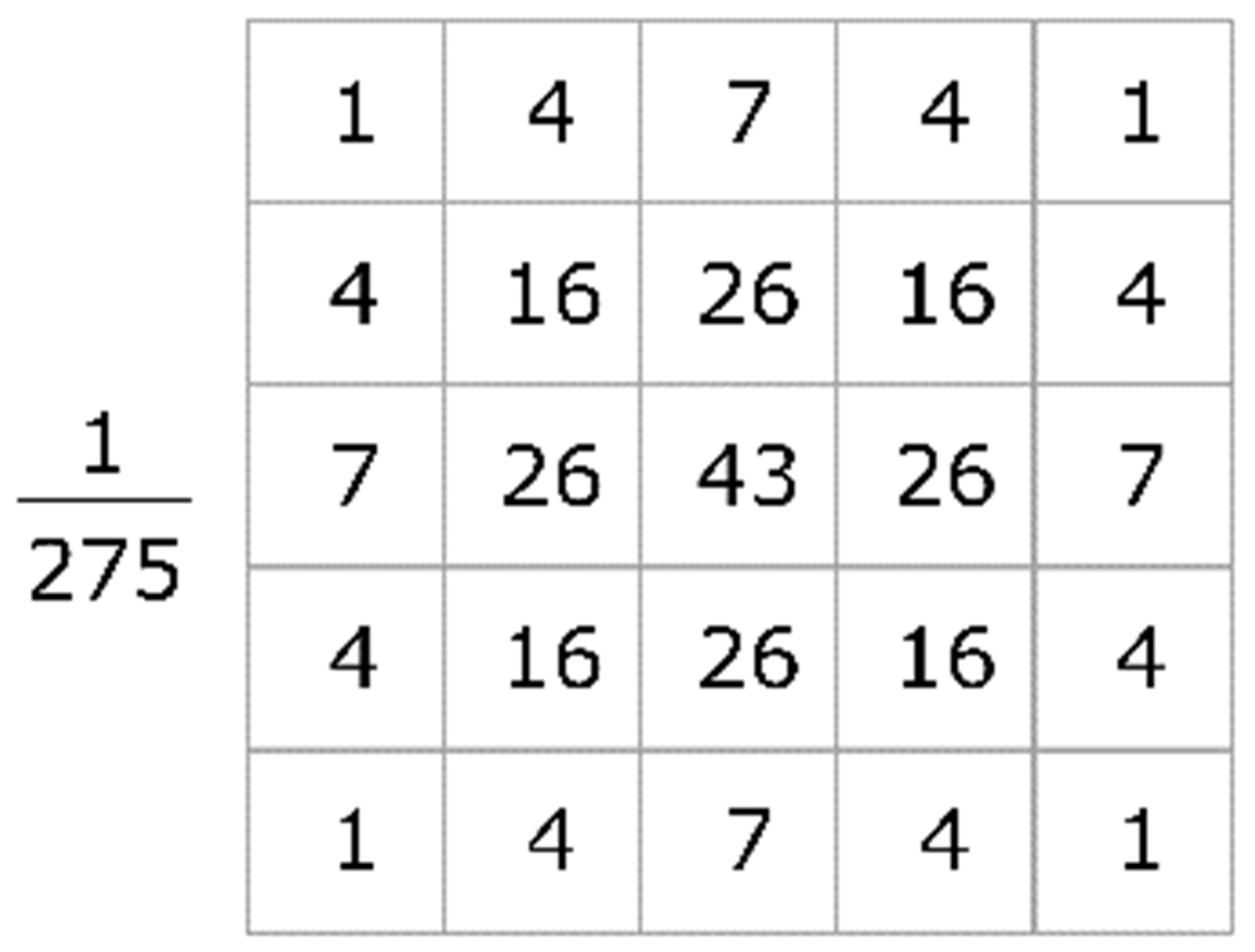
The Gaussian smoothing filter is a specialized filter based on a 2D convolution operator used to reduce Gauss noise at certain locations in an image. Unlike the mean filter, the Gaussian filter uses convolutional kernel to represent the approximation of Gaussian distribution (“bell-shaped” hump) by forming a convolution matrix with the help of values from this distribution [19]. The distribution is non-zero everywhere in theory, requiring an arbitrarily large convolution kernel, but it is essentially zero beyond around three standard deviations from the mean in practice, allowing us to terminate the kernel at this point. The average value is 0, as noise amplitude distribution is normal; thus, the Gaussian filter forms this kernel to remove noise or blur the image with function in the two dimensions given in (1), where, y and x refer to Cartesian coordinates of the image, that is, the vertical and horizontal lengths from the origin, respectively, and the standard deviation of Gaussian function is depicted by σ (sigma). An appropriate sample integer-valued convolution kernel that approximates a Gaussian with a sigma of 1.0 is shown in Figure 4.

$$G\left(x,y\right)=\frac{1}{2\pi {\sigma }^2}{e}^{-\frac{x^2+y^2}{2{\sigma }^2}}$$

(1)

Choosing the center value in mask to approximate a Gaussian may generate inaccurate results, as Gaussian varies non-linearly throughout the pixels; thus, it integrates it over the entirety of the pixels, as shown in Figure 4, with 275 as mask sum. Later, the formulated normalized convolutional matrix is applied to the original image represented by matrix, thus forming new set of pixels with the weighted average of the surrounding pixels.

2.2. Feature-Extraction Techniques

Due to diversified data with huge sizes, the researchers of CV and the deep learning community suggested different methods and tools to reduce the dimensionality of data for performance enhancement while also performing classification, such as backward feature elimination, RF, LDA, and PCA. This study employed LDA and PCA as feature-extraction techniques to obtain the best features from the three datasets of filtered images, which have effective information that is then used to train the machine learning models separately for each dataset.

2.2.1. LDA

LDA is a transformation technique for dimensionality reduction and feature extraction formulated by R.A. Fisher in 1936 [20]. It was initially used for two-class classification problems, which, later in 1948, were generalized for multi-class classification tasks. The statistical approach is nearer to PCA (which is described in succeeding sub-section); however, instead of looking for component axes, which maximize the variance, it also determines the axes that maximize segregation between two or more classes. Unlike PCA, it performs supervised tasks by determining the optimal linear discriminants that minimize the variability within classes but maximize variability between multiple classes. LDA works as follows:

• For each class, determine n-dimensional mean vectors;
• Calculate scatter matrices;
• For each scatter matrix, determine eigenvectors ($e_1, e_2,e_3, \dots , e_n$) and respective eigenvalues (${\lambda }_1, {\lambda }_2,{\lambda }_3, \dots , {\lambda }_n$);
• Take first $l$ eigenvectors from descending sort vectors to form matrix $W$ having $n\times l$ dimensions;
• Create new sub-space $Y=W\times X$ using $n\times l$ eigenvector matrix, where $Y$ corresponds to new subspace ($k\times l$)-dimensional samples, and $X$ represents $k$ samples in ($k\times n$)-dimensional matrix.

Thus, it transforms the data from higher-dimensional space to lower-dimensional, which significantly reduces the computational cost of the model.

2.2.2. Kernel PCA

Kernel PCA is a statistical method broadly followed to derive crucial information by evaluating variables’ dependency in original dataset. It transforms the inter-correlated data to principal components containing a set of orthogonal variables [21]. It drastically reduces dataset dimensionality in an unsupervised manner and increases interpretability while minimizing information loss [22]. After orthogonal transformation, each principal component in a new set attains a certain variance (first component with highest variance) under the constraint that is orthogonal to the preceding components.

Assuming dataset images are stored in a 2D matrix, X(N, M), while N < M, N corresponds to total samples, and M refers to entire pixels after masking, and N < M. The basic idea in PCA is to reduce this dimensionality by applying linear transformation U(M, L) to form a new matrix, Z(N, L), where L < M, while preserving plenty of information from original data X.

$$Z=U^{T}X$$

(2)

The information is represented by covariance matrix S(L, L):

$$S_Z=\frac{1}{N}{Z}^{T}Z$$

(3)

As the goal is dimensionality reduction while losing minimum information, optimization thus yields:

$$\underset{U}{\max }{S}_z=\underset{U}{\max }{U}^T{S}_{X}U$$

(4)

This maximization has no upper bound on U. Every vector in this matrix has unit magnitude U^TU = 1. Applying Lagrange to this optimization introduces eigenvector equation with Lagrange multiplier, λ:

$$S_{X}U=\lambda U$$

(5)

Solving this S_X in (8), with a covariance matrix of size M × M and with eigen-decomposition (matrix diagonalization) of covariance matrix as X, yields S as:

$$S=P D P^{-1}$$

(6)

where P is the eigenvector matrix, and D is diagonal matrix consisting eigenvalues. Thus, the total variance TV after transformation is the sum of eigenvalues as:

$$TV={\displaystyle \sum }_{i=1}^M{\lambda }_i$$

(7)

For L-highest eigenvector features among M vectors, the retained variance RV is calculated by:

$$RV={\displaystyle \sum }_{i=1}^L{\lambda }_i$$

(8)

Thus, the percentage of features retained, FR, out of real data is formulated using:

$$FR=\frac{{{\displaystyle \sum }}_{i=1}^L{\lambda }_i}{{{\displaystyle \sum }}_{i=1}^M{\lambda }_i}$$

(9)

Simplifying the above equations, the techniques examine the dataset in each dimension by calculating its mean. It then determines covariance matrix, eigenvector, and corresponding value pairs with the help of matrix diagonalization. Finally, the eigenvalues are sorted in descending matter; thus, top L value pairs preserve effective features having the maximum amount of information. As normal PCA fails to create a hyperplane when data are non-linear, this study thus exploited kernel PCA that performs kernel-trick to convert data into higher dimensionality where it is separable.

2.3. Classification Methods

This part of the study outlines the deep learning models implemented to identify coronavirus patients. The section presents an overview of CNN, SVM, and LG models exploited to achieve the clinical purpose of COVID-19 classification with healthy individuals.

2.3.1. CNN

CNNs [23] have shattered the mold and climbed to the throne to become the most state-of-the-art approach for computer vision [24]. CNNs are by far the most common kind of neural network among various types of neural networks, such as recurrent neural networks (RNN), long–short-term memory (LSTM), artificial neural networks (ANN), and so on. Within the realm of visual data, these CNN models may be found constantly. They do very well in computer vision tasks such as image categorization, object identification, and image recognition, amongst other computer vision tasks, via three commons layers: pooling, dense, and convolutional layers (CL), as seen in Figure 5. Each layer plays a significant role in classification. For example, CLs transforms input data to meaningful representation by connecting neurons having similar characteristics with weight, w, and bias, b, to determine the weighted sums of all activations of a layer, as given below.

$$\sigma \left(\left[\begin{array}{ccc}{w}_{0,0}& \cdots & w_{0,n}\\ ⋮& \ddots & ⋮\\ w_{k,0}& \cdots & w_{k,n}\end{array}\right]\left[\begin{array}{c}{a}_0^{\left(0\right)}\\ ⋮\\ a_n^{\left(0\right)}\end{array}\right]+\left[\begin{array}{c}{b}_0\\ ⋮\\ b_n\end{array}\right]\right)=\left[\begin{array}{c}{a}_0^{\left(1\right)}\\ ⋮\\ a_k^1\end{array}\right]$$

(10)

where σ refers sigmoid to normalize the resultant. Later, the resultant CL is fed to a rectified linear unit (ReLU) to perform elementwise activation with the help of the following [25]:

$$ReLU=\max \left(0,x\right)$$

(11)

The sub-sampling of the feature maps is the primary duty of the pooling layer, and it is the function that is accountable for reducing the overall spatial extent of the converged feature [26]. The max pooling method is a pooling approach that selects the most significant and biggest element from the range of the filter’s feature map.

In machine learning models, the last layers are often fully connected layers. This means that every node included inside a fully connected layer is directly related to every other node included within the level directly before it and the level directly following it. The softmax function is often employed (for more than two-class classification tasks) as the activation function in the output layer of neural network models that anticipate multinomial probability distributions. The mathematical representation given below is applied to each element, $s$:

$$f{\left(s\right)}_i=\frac{e^{s_i}}{{{\displaystyle \sum }}_j{e}^{s_j}}$$

(12)

where s_j refers to output scores inferred for each class in $C$.

2.3.2. SVM

Due to its classification performance, robustness, and neutrality towards the input data type, SVM has garnered a growing amount of interest [27]. As an application of statistical learning theory, SVM addresses problems with huge margins of classification by selecting a subset and referring to these as support vectors. It creates a separating hyperplane to maximize the margin that is free of training data. SVM, being a supervised machine learning approach, can be applied to problems involving either classification or regression.

In SVM, gamma, C, and kernel are three of the most important parameters [28]. Gamma specifies the extent to which the effect of single training instances leads to biased outcomes. A low value of gamma will provide a linear boundary, which may lead to underfitting, while a high value of the gamma will be a very compact boundary and conduct highly rigorous classification, which may lead to overfitting. Both of these outcomes are possible depending on the value of gamma. C manages the cost of misclassifications, which may be associated with any positive real value. When using a small C, the cost of misclassification is kept to a minimum, but using a large C, the cost raises significantly. On the other hand, kernel refers to the collection of mathematical functions used by SVM algorithms. Linear, radial basis function (RBF), and polynomial kernels are the three different types of kernels. This study uses polynomial kernel, as it is widely used to identify the similarity of training instances in a feature set throughout polynomials of the original variables, which enables the learning of non-linear models.

2.3.3. LG

Estimating the probability that a given instance belongs to a certain class is a popular use of a statistical technique known as LG, which is sometimes known as logit regression. If the estimated probability is more than 50 percent, then the model can predict that the instance belongs to that class and otherwise to another class. Most models, such as the linear regression model, compute a weighted sum of the input features (as well as a bias term). However, LG models output the logistic of the result rather than the result itself by determining the probability, $\widehat{y}$, as given below for an instance $x$:

$$\widehat{y}=h_{\theta }\left(x\right)=\sigma \left(x^T\theta \right).$$

(13)

The logistic function, noted as $\sigma (.)$, is a sigmoid function that returns a number in the range of 0 to 1 using the following:

$$\sigma \left(t\right)=\frac{1}{1+e^{-t}}.$$

(14)

After the logistic regression model has determined the probability that $x$ belongs to the positive class, it is then able to make its prediction, denoted by $\widehat{p}$, with relative ease:

$$\widehat{p}=0 if \widehat{y}<0.5 \mathrm{and} \widehat{p}=1 if \widehat{y}\ge 0.5$$

(15)

3. Results and Discussion

Besides classifying radiography imaging as COVID-19-negative or -positive cases, the research aims to investigate the symmetry of imaging content by exploiting various combinations of three filtering approaches and two feature-extraction techniques with three machine-learning-based classifiers. Basically, each image passes through three stages: image filtering, feature extraction, and classification. In the proposed scheme, the images are fed to each filter individually to remove unwanted noise. Later, each feature-extraction technique extracts useful features from filtered images. Finally, a classifier processes extracted features to predict the result based on its training. The image filtering approaches include conservative smoothing filter, Crimmins speckle removal filter, and Gaussian smoothing filter, whereas feature-extraction techniques include LDA and PCA, while the classification stage exploited three different classifiers (CNN, SVM, and LG).

Extensive experiments were performed by exploiting various other approaches and techniques, such as median filter, frequency filter, mean filter, and Laplacian of Gaussian filter as image filtering, t-SNA and RF as feature selection, DT and LSTM as classification, etc.; however, the paper only presents the results of those techniques that accomplished a high performance. Moreover, the research is widened by repeating each experiment 10 times to ensure the correctness and performance accuracy of each combinational structure (filters, feature selectors, and classifiers). The experimental task was executed on Intel^® Core i5 11th Generation Processor Intel^® Xeon^® CPU E3-1231 3.40 GHz processor having a RAM of 16 GB. The software used includes Jupyter Notebook having Keras packages with Python 3.8. In addition, the system contains Intel^® Iris^® X^e graphics.

For experimental setup, the study formed a dataset by acquiring radiography images from two sources, containing 7348 chest X-ray images. A division of 20–80% was made in the compiled dataset as test and train sets, respectively. Furthermore, 20% of the training data was further used for validation to avoid overfitting and underfitting issues, and more details can be found in

Table 2. Dataset split information.

Cases	Dataset	Training Set	Validation Set	Testing Set
COVID-19	3674	2351	588	735
Healthy Individuals	3674	2351	588	735
Total	7348	4702	1176	1470

. The images varied in sizes depending upon the resolution of capturing devices; thus, to maintain uniformity, each image was resized to a fixed shape (height × width: 256 × 256) having three channels. Moreover, to handle the model’s fitting issues, the study employed five-fold cross-validation in the training phase. The selection of five-fold was based after testing experiments with various other folds.

3.1. Noise Removal

The study exercised conservative smoothing filter, Crimmins speckle removal filter, and Gaussian separately on each chest X-ray raw image to enhance its quality by removing unnecessary noise. Three new datasets were obtained after filtering the original dataset with these three image filtering approaches individually.

To form the first dataset (cnsf-dataset), a conservative smoothing filter was applied on images to have more subtle effect by adjusting the intensity of the central pixel based on the maximal value within the window frame. Figure 6a depicts a raw image and its corresponding filtered image obtained using the conservative smoothing filter. To form another filtered dataset (csrf-dataset), the study employed Crimmins speckle removal filter (characteristics described in Section 2) on all images of the original dataset. It removed speckle noise; however, it also blurred some of the edges. Lastly, a third dataset (gsf-dataset) was generated by exploiting Gaussian smoothing filter, having a kernel size of 5 × 5. Moreover, at runtime, it automatically determined the standard deviation in x- and y-directions based on kernel size. The Gaussian smoothing filter successfully removed some noise and retained more information and edges.

3.2. Feature Extraction

Training machine-learning-based classifiers directly with raw images often yields poor results because of information redundancy and high data rate. Thus, feature extraction is usually preferred before applying machine learning directly on raw data, as it determines the most discriminating characteristics in an image that a machine learning algorithm can easily consume to produce better outcomes. This study investigated several feature-extraction approaches; however, it only presents the analysis of approaches with most optimal results, which includes LDA and PCA.

Each dataset (cnsf-dataset, csrf-dataset, and gsf-dataset) is fed to LDA and PCA separately to automatically extract the most relevant representations and eliminate redundant information in order to speed up the learning and generalization steps in the machine learning process.

3.2.1. Using LDA

LDA is a potential candidate for employment for feature extraction to retain highly informative features. It works in a similar fashion as PCA except being a supervised algorithm. Thus, class labels are also provided along with filtered images while performing fit operation in LDA to guarantee class separability by maximizing the component axes for class separation. This study determines the top features by looking at the direction of maximum separability as a function of the number of components. To evaluate the effect of the linear feature-extraction approach via LDA on the proposed classification models, only prominently features from each filtered image are selected that achieved maximum separability scores in LDA.

Table 3. Number of features extracted by linear discriminant analysis (LDA) for each filtered dataset.

Set. No.	Variance Attained	Features Extracted by LDA for Each Filter
		Conservative	Crimmins	Gaussian
1	0.99	222	225	216
2	0.97	186	180	174
3	0.95	144	150	150
4	0.90	96	96	81
5	0.85	48	48	48

tabulates the number of features that are formulated from each dataset through LDA for training the proposed classification models.

3.2.2. Using PCA

Unlike LDA, PCA is an unsupervised algorithm where classes or labels are not provided to find optimal features. Before proceeding further, in order to obtain better results, the proposed scheme performed scaling and normalized the pixel values of each image with unit scaling by setting $variance=1$ and $mean=0$ and the images. Later, kernel PCA performed orthogonal transformation to find the direction of maximum variation in the given data in order to detect and retain representations possessing important information. The kernel PCA provided sorted relevant representations (principal components) in decreasing order based on eigenvalues. This study determined the top principal components by looking at cumulative explained variance ratio as a function of the number of components. In other words, it determined out how much variance is contained within the first N principal components. Thus, the study considered feature sets (principal components) that equate to variance of 0.99, 0.97, 0.95, 0.90, and 0.85 as summarized in

Table 4. Number of features extracted by principal component analysis (PCA) for each filtered dataset.

Set. No.	Variance Attained	Features Selected by PCA for Each Filter
		Conservative	Crimmins	Gaussian
1	0.99	216	216	210
2	0.97	168	174	180
3	0.95	108	105	105
4	0.90	90	84	81
5	0.85	48	45	48

. Later, each extracted feature set was utilized separately to train the machine learning models for diagnostic purposes.

3.3. Classification

This study performed extensive experiments to investigate several machine learning and deep learning approaches, such as CNN, SVM, LG, DT, RF, LSTM, and Bi-LSTM, etc.; however, this paper only presents the analysis of approaches with the most optimal results, which include CNN, SVM, and LG.

3.3.1. Using CNN

The study proposes a CNN model (see Figure 5) to classify radiography chest images as COVID-19-positive or -negative cases. The size (height × width × 3) of the input layer of the proposed model varies depending on variations in height and width of the generated feature sets. It utilized an Adam optimizer with a learning rate of 0.001, beta_2 = 0.999, beta_1 = 0.9, and amsgrad to false. Augmentation on the fly technique was used, whereas epochs and batch size were set to 30 and 10, respectively. A detailed network topology and hyperparameters of the proposed CNN model can found in

Table 5. The proposed convolutional neural network topology.

CNN Proposed Topology
Dataset	Convolution Layers				Fully Connected Layers
	Kernel Size	ReLU	Max Pooling	Dropout	No. of Neurons	Function	Dropout
CRD andACCDI	3 × 3 × 32	Yes	No	No
	3 × 3 × 32	Yes	2 x 2	Yes (10%)
	5 × 5 × 64	Yes	No	No
	5 × 5 × 64	Yes	2 x 2	No
	5 × 5 × 64	Yes	NO	Yes (15%)	128	ReLU	Yes (30%)
					2	Sigmoid	No
Other Parameters
Batch size	Steps (iterations)	Epochs	Learning rate	Optimizer
10	100	30	0.001	Adam

.

The proposed model utilized feature sets extracted in the previous section to train and test the model, separately. For instance, a feature set obtained from cnsf-dataset that has a variance of 0.99 was given to the proposed CNN classification model. Later, the model was tested, and performance was analyzed as given in

Table 6. The performance evaluation of convolutional neural network (CNN) model with linear discriminant analysis.

Filtering Type	VR	CNN
		Precision			Sensitivity			F1-Score
		Normal	CVD-19+	Overall	Normal	CVD-19+	Overall	Normal	CVD-19+	Overall
Conservative Smoothing	1	0.992	0.995	0.993	0.995	0.992	0.993	0.993	0.993	0.993
	0.99	0.982	0.968	0.975	0.967	0.982	0.975	0.975	0.975	0.975
	0.97	0.993	0.997	0.995	0.997	0.993	0.995	0.995	0.995	0.995
	0.95	0.997	0.995	0.996	0.996	0.997	0.997	0.997	0.997	0.997
	0.90	0.997	0.995	0.996	0.996	0.997	0.997	0.997	0.997	0.997
	0.85	0.992	0.996	0.994	0.996	0.992	0.994	0.994	0.994	0.994
Crimmins Speckle Removal	1	0.972	0.977	0.974	0.977	0.972	0.974	0.974	0.974	0.974
	0.99	0.976	0.983	0.980	0.984	0.976	0.980	0.980	0.980	0.980
	0.97	0.986	0.989	0.988	0.990	0.987	0.988	0.988	0.988	0.988
	0.95	0.988	0.990	0.989	0.990	0.988	0.989	0.989	0.989	0.989
	0.90	0.977	0.980	0.978	0.980	0.977	0.978	0.978	0.978	0.978
	0.85	0.973	0.969	0.971	0.969	0.973	0.971	0.971	0.971	0.971
Gaussian	1	0.974	0.962	0.968	0.962	0.974	0.968	0.968	0.968	0.968
	0.99	0.951	0.954	0.952	0.954	0.951	0.952	0.952	0.952	0.952
	0.97	0.960	0.957	0.958	0.956	0.960	0.958	0.958	0.958	0.958
	0.95	0.973	0.966	0.969	0.966	0.973	0.970	0.969	0.969	0.969
	0.90	0.964	0.961	0.963	0.961	0.965	0.963	0.963	0.963	0.963
	0.85	0.950	0.952	0.951	0.952	0.950	0.951	0.951	0.951	0.951

VR, variance retained; CVD-19+, COVID-19-positive cases.

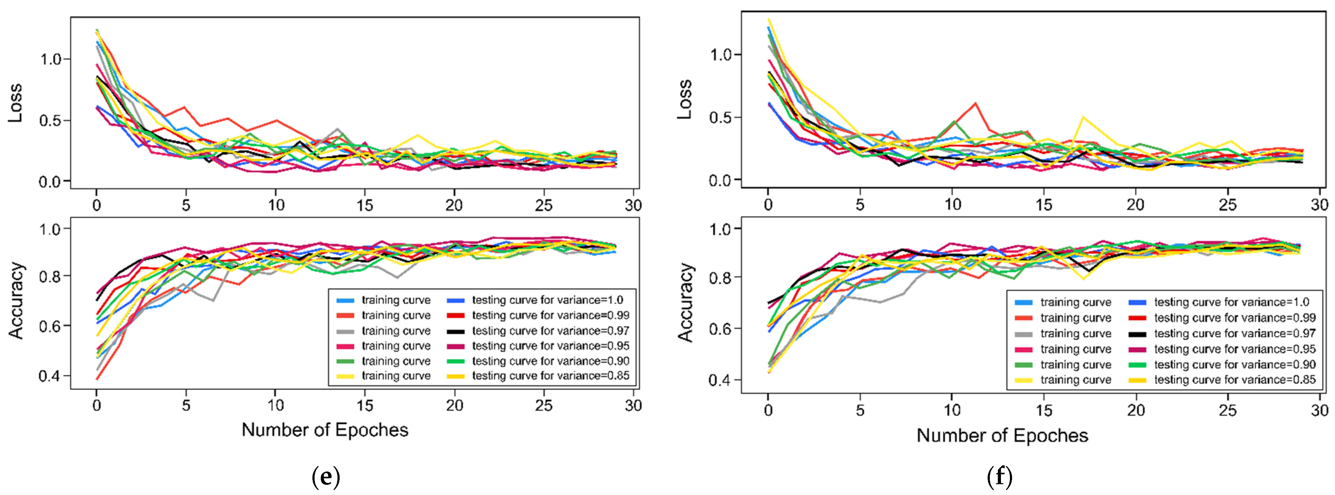
. Similarly, all feature sets obtained using LDA and PCA of the three datasets (cnsf-dataset, csrf-dataset, and gsf-dataset) were used individually to train a separate CNN model with the same configuration. Figure 6a,c,e depicts detailed performance curves (accuracy and loss) for each combinational filtering scheme with LDA, while Figure 6b,d,f reflects performance curves for PCA when combined with different filters. The performance of the proposed CNN model was measured using several metrices as shown in Table 6 and

Table 7. The performance evaluation of convolutional neural network (CNN) model with kernel principal component analysis.

Filtering Type	VR	CNN
		Precision			Sensitivity			F1-Score
		Normal	CVD-19+	Overall	Normal	CVD-19+	Overall	Normal	CVD-19+	Overall
Conservative Smoothing	1	0.992	0.995	0.993	0.995	0.992	0.993	0.993	0.993	0.993
	0.99	0.992	0.988	0.990	0.988	0.992	0.990	0.990	0.990	0.990
	0.97	0.986	0.978	0.982	0.978	0.986	0.982	0.982	0.982	0.982
	0.95	0.997	0.991	0.994	0.990	0.997	0.994	0.994	0.994	0.994
	0.90	0.984	0.980	0.982	0.980	0.984	0.982	0.982	0.982	0.982
	0.85	0.987	0.963	0.975	0.962	0.988	0.975	0.975	0.975	0.975
Crimmins Speckle Removal	1	0.972	0.977	0.974	0.977	0.972	0.974	0.974	0.974	0.974
	0.99	0.976	0.981	0.978	0.981	0.976	0.978	0.978	0.978	0.978
	0.97	0.985	0.977	0.981	0.977	0.985	0.981	0.981	0.981	0.981
	0.95	0.988	0.980	0.984	0.980	0.988	0.984	0.984	0.984	0.984
	0.90	0.978	0.972	0.975	0.971	0.978	0.975	0.975	0.975	0.975
	0.85	0.971	0.962	0.967	0.962	0.971	0.967	0.967	0.967	0.967
Gaussian	1	0.974	0.962	0.968	0.962	0.974	0.968	0.968	0.968	0.968
	0.99	0.952	0.949	0.950	0.948	0.952	0.950	0.950	0.950	0.950
	0.97	0.939	0.926	0.932	0.925	0.940	0.933	0.932	0.933	0.933
	0.95	0.946	0.933	0.940	0.932	0.947	0.939	0.939	0.940	0.939
	0.90	0.931	0.921	0.926	0.920	0.932	0.926	0.925	0.926	0.926
	0.85	0.939	0.919	0.929	0.917	0.940	0.929	0.928	0.929	0.929

VR, variance retained; CVD-19+, COVID-19-positive cases.

for classification when combined with LDA and PCA, respectively.

Results show that CNN performed well when conservative smoothing filter was employed along with LDA, as it attained 99.6% precision, 99.7% sensitivity, and 99.7% f1-score.

3.3.2. Using SVM

Besides other machine-learning-based classifiers, this study also analyzed the SVM on the given data. The feature sets extracted from filtered images using LDA and kernel PCA were fed to the SVM model separately. The parameters of proposed SVM were fine-tuned empirically, such as the penalty parameter, and C for the error term was set to 1 to handle error, whereas gamma was set auto. Moreover, it exploited both polynomial kernel for training inside a feature set across polynomials of original variables and RBF for non-linear modeling (see

Table 8. Hyperparametric values for the proposed support vector machine model.

Hyperparameter	Value
C	1
Kernel	Poly and RBF
Gamma	Auto

).

Table 9. The performance evaluation of the support vector machine (SVM) model with linear discriminant analysis.

Filtering Type	VR	SVM
		Precision			Sensitivity			F1-Score
		Normal	CVD-19+	Overall	Normal	CVD-19+	Overall	Normal	CVD-19+	Overall
Conservative Smoothing	1	1.0	0.999	0.999	0.999	1.0	0.999	0.999	0.999	0.999
	0.99	0.996	0.992	0.994	0.992	0.996	0.994	0.994	0.994	0.994
	0.97	0.995	0.997	0.996	0.997	0.995	0.996	0.996	0.996	0.996
	0.95	1.0	0.997	0.999	0.999	1.0	0.999	0.999	0.999	0.999
	0.90	1.0	0.997	0.999	0.999	1.0	0.999	0.999	0.999	0.999
	0.85	1.0	0.997	0.999	0.999	1.0	0.999	0.999	0.999	0.999
Crimmins Speckle Removal	1	0.988	0.982	0.985	0.982	0.988	0.985	0.985	0.985	0.985
	0.99	0.981	0.981	0.981	0.981	0.981	0.981	0.981	0.981	0.981
	0.97	0.990	0.976	0.983	0.976	0.990	0.983	0.983	0.983	0.983
	0.95	0.973	0.985	0.979	0.985	0.973	0.979	0.979	0.979	0.979
	0.90	0.974	0.962	0.968	0.962	0.974	0.968	0.968	0.968	0.968
	0.85	0.996	0.983	0.989	0.982	0.996	0.989	0.989	0.989	0.989
Gaussian	1	0.954	0.964	0.959	0.967	0.954	0.959	0.959	0.959	0.959
	0.99	0.959	0.964	0.962	0.965	0.959	0.962	0.962	0.962	0.962
	0.97	0.974	0.970	0.972	0.970	0.972	0.972	0.972	0.972	0.972
	0.95	0.975	0.966	0.971	0.966	0.975	0.971	0.971	0.971	0.971
	0.90	0.969	0.948	0.959	0.947	0.970	0.959	0.958	0.958	0.958
	0.85	0.977	0.974	0.976	0.974	0.977	0.975	0.975	0.976	0.976

VR, variance retained; CVD-19+, COVID-19-positive cases.

lists the results obtained for diagnosing COVID-19 patients or healthy individuals using LDA, while

Table 10. The performance evaluation of the support vector machine (SVM) model with kernel principal component analysis.

Filtering Type	VR	SVM
		Precision			Sensitivity			F1-Score
		Normal	CVD-19+	Overall	Normal	CVD-19+	Overall	Normal	CVD-19+	Overall
Conservative Smoothing	1	1.0	0.999	0.999	0.999	1.0	0.999	0.999	0.999	0.999
	0.99	0.974	0.953	0.963	0.952	0.974	0.963	0.963	0.964	0.963
	0.97	0.989	0.980	0.984	0.980	0.989	0.984	0.984	0.984	0.984
	0.95	0.966	0.960	0.963	0.961	0.966	0.963	0.963	0.963	0.963
	0.90	0.974	0.966	0.970	0.966	0.974	0.970	0.970	0.970	0.970
	0.85	0.973	0.968	0.970	0.967	0.973	0.970	0.970	0.970	0.970
Crimmins Speckle Removal	1	0.988	0.982	0.985	0.982	0.988	0.985	0.985	0.985	0.985
	0.99	0.988	0.972	0.980	0.971	0.988	0.980	0.979	0.980	0.980
	0.97	0.980	0.976	0.978	0.976	0.980	0.980	0.978	0.978	0.978
	0.95	0.960	0.973	0.966	0.973	0.960	0.966	0.966	0.966	0.966
	0.90	0.981	0.965	0.973	0.965	0.981	0.973	0.973	0.973	0.973
	0.85	0.981	0.965	0.973	0.965	0.981	0.973	0.973	0.973	0.973
Gaussian	1	0.954	0.964	0.959	0.967	0.954	0.959	0.959	0.959	0.959
	0.99	0.946	0.952	0.949	0.952	0.946	0.949	0.949	0.949	0.949
	0.97	0.946	0.937	0.942	0.936	0.947	0.941	0.941	0.942	0.941
	0.95	0.960	0.954	0.958	0.954	0.961	0.957	0.957	0.958	0.957
	0.90	0.944	0.933	0.939	0.932	0.946	0.939	0.938	0.939	0.939
	0.85	0.940	0.931	0.935	0.931	0.940	0.935	0.935	0.936	0.935

VR, variance retained; CVD-19+, COVID-19-positive cases.

shows the proposed scheme’s performance when PCA is combined with three different image filtering models. It is evident from these tables that the SVM model performed better when combined with LDA and conservative smoothing filter by achieving an overall precision, recall, and f1-score of 99.9% each.

3.3.3. Using LG

Similar to CNN and SVM, the extracted feature sets were given to LG for training the classifier. After empirically calculating and setting the parametric values (see

Table 11. Hyperparametric values for the proposed logistic regression model.

Hyperparameter	Value
CV	5
Random state	1234
Class weight	Balanced
Solver	Liblinear
Verbose	1
No. of jobs	−1
Maximum iteration	400

) for LG, the model was trained with five-fold cross-validation, having a single verbose and balanced class weight.

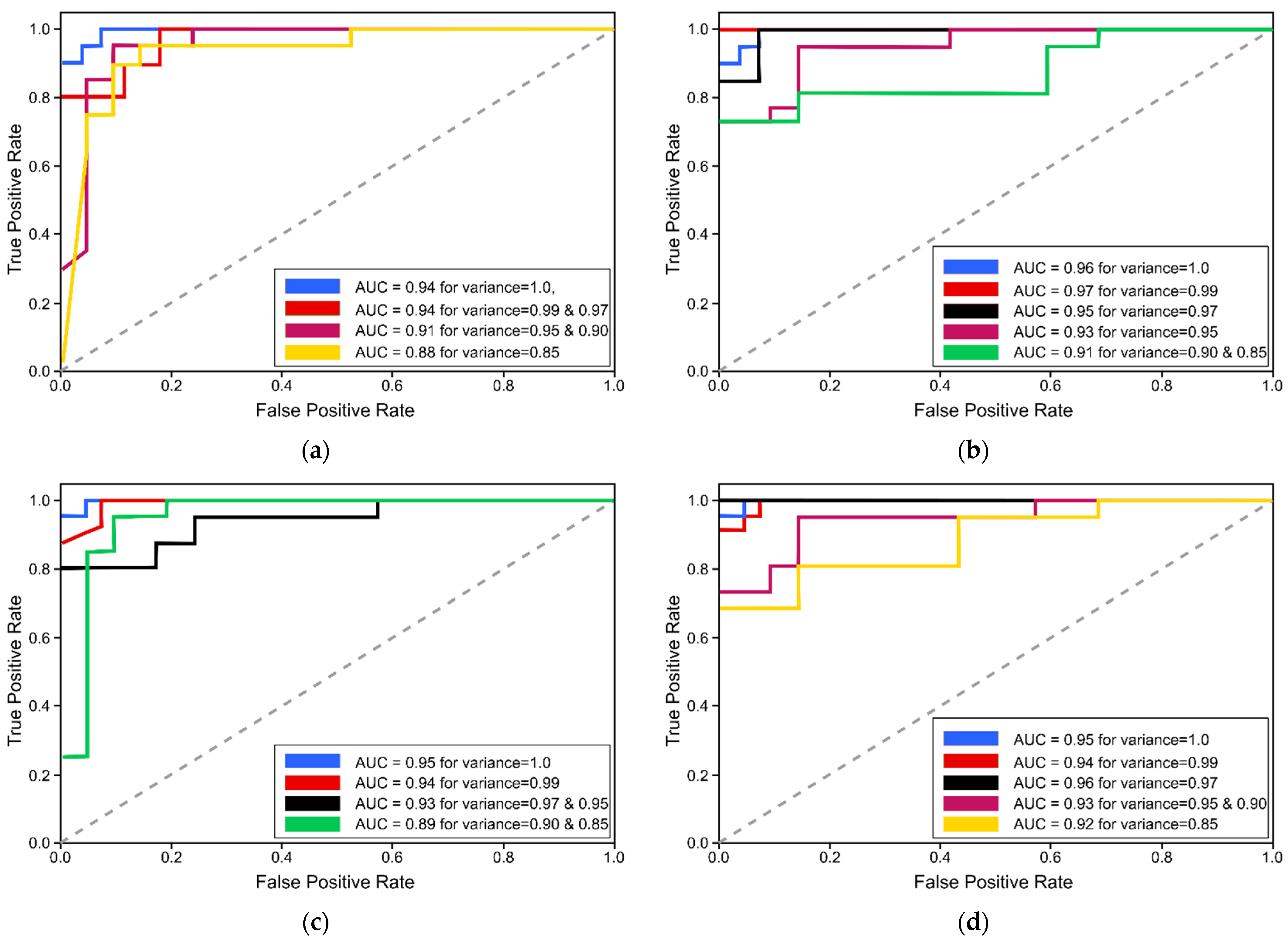
Later, performance metrices were calculated for each trained model on different feature sets. Figure 7 illustrates the receiver-operating characteristics (ROC) curves to analyze the performance of proposed LG schemes when trained with extracted feature sets of varying variances using LDA and PCA. Moreover,

Table 12. The performance evaluation of logistic regression (LG) model with linear discriminant analysis.

Filtering Type	VR	LG
		Precision			Sensitivity			F1-Score
		Normal	CVD-19+	Overall	Normal	CVD-19+	Overall	Normal	CVD-19+	Overall
Conservative Smoothing	1	0.963	0.955	0.959	0.955	0.963	0.959	0.959	0.959	0.959
	0.99	0.944	0.933	0.938	0.932	0.944	0.938	0.938	0.938	0.938
	0.97	0.946	0.935	0.941	0.937	0.947	0.941	0.940	0.941	0.941
	0.95	0.925	0.899	0.912	0.895	0.928	0.911	0.910	0.913	0.912
	0.90	0.927	0.896	0.911	0.893	0.929	0.911	0.909	0.912	0.911
	0.85	0.869	0.887	0.878	0.890	0.865	0.878	0.879	0.876	0.878
Crimmins Speckle Removal	1	0.951	0.958	0.954	0.959	0.951	0.954	0.955	0.954	0.954
	0.99	0.938	0.941	0.939	0.941	0.937	0.939	0.940	0.939	0.939
	0.97	0.936	0.921	0.928	0.920	0.937	0.929	0.928	0.929	0.929
	0.95	0.930	0.923	0.926	0.918	0.934	0.926	0.924	0.928	0.926
	0.90	0.902	0.883	0.893	0.880	0.905	0.893	0.891	0.894	0.893
	0.85	0.899	0.880	0.889	0.878	0.901	0.889	0.888	0.890	0.889
Gaussian	1	0.926	0.941	0.933	0.942	0.925	0.933	0.934	0.933	0.933
	0.99	0.903	0.918	0.910	0.920	0.901	0.910	0.911	0.909	0.910
	0.97	0.919	0.896	0.907	0.893	0.921	0.907	0.905	0.908	0.908
	0.95	0.897	0.877	0.887	0.863	0.908	0.885	0.879	0.892	0.886
	0.90	0.872	0.873	0.873	0.873	0.872	0.873	0.873	0.873	0.873
	0.85	0.863	0.851	0.857	0.849	0.865	0.857	0.856	0.858	0.857

VR, variance retained; CVD-19+, COVID-19-positive cases.

presents the performance evaluation metrices of LG model when trained and tested with features extracted using LDA, while

Table 13. The performance evaluation of the logistic regression (LG) model with kernel principal component analysis.

Filtering Type	VR	LG
		Precision			Sensitivity			F1-Score
		Normal	CVD-19+	Overall	Normal	CVD-19+	Overall	Normal	CVD-19+	Overall
Conservative Smoothing	1	0.963	0.955	0.959	0.955	0.963	0.959	0.959	0.959	0.959
	0.99	0.965	0.971	0.968	0.971	0.965	0.968	0.968	0.968	0.968
	0.97	0.946	0.949	0.948	0.950	0.946	0.948	0.948	0.948	0.948
	0.95	0.931	0.933	0.932	0.933	0.931	0.932	0.932	0.932	0.932
	0.90	0.927	0.896	0.911	0.893	0.929	0.911	0.909	0.912	0.911
	0.85	0.920	0.896	0.908	0.893	0.922	0.907	0.906	0.909	0.907
Crimmins Speckle Removal	1	0.951	0.958	0.954	0.959	0.951	0.954	0.955	0.954	0.954
	0.99	0.938	0.950	0.944	0.951	0.937	0.944	0.945	0.944	0.944
	0.97	0.953	0.960	0.956	0.961	0.952	0.956	0.957	0.956	0.956
	0.95	0.939	0.926	0.933	0.922	0.942	0.932	0.931	0.934	0.932
	0.90	0.938	0.927	0.933	0.927	0.938	0.937	0.932	0.933	0.933
	0.85	0.934	0.908	0.921	0.905	0.936	0.920	0.919	0.922	0.920
Gaussian	1	0.926	0.941	0.933	0.942	0.925	0.933	0.934	0.933	0.933
	0.99	0.935	0.922	0.929	0.921	0.936	0.929	0.928	0.929	0.929
	0.97	0.938	0.920	0.929	0.918	0.939	0.929	0.928	0.929	0.929
	0.95	0.902	0.919	0.911	0.914	0.908	0.911	0.908	0.913	0.911
	0.90	0.892	0.890	0.891	0.890	0.893	0.891	0.891	0.891	0.891
	0.85	0.877	0.885	0.881	0.886	0.876	0.881	0.882	0.880	0.881

VR, variance retained; CVD-19+, COVID-19-positive cases.

outlines the performance metrices of LG classification model when used along with the PCA feature-extraction technique. Results prove that LG could not meet the performance as compared with SVM and CNN models. However, it still achieved 95.9% f1-score, 95.9% sensitivity, and 95.9% precision on test set when trained with feature sets extracted by PCA using conservative smoothing filter.

3.4. Performance Analysis and Discussion

Besides this, the study also exploited the proposed classification model without employing image filtering and feature-extraction techniques.

Table 14. The performance metrices of convolutional neural network (CNN), support vector machine (SVM), and logistic regression (LG) with and without image filtering and feature-extraction techniques for detecting COVID-19 cases in the gathered dataset.

Scheme/Technique	Accuracy (%)
	CNN	SVM	LG
Without image filtering and feature-extraction techniques	96.93	97.07	92.61
With image filtering and feature-extraction techniques	99.32	99.93	95.92

shows the performance metrices obtained when the proposed classification models are trained directly with the original dataset after initial preprocessing, such as image resizing, etc. It is evident from Table 14 that the proposed amalgam scheme of combining image filtering with feature-extraction methods significantly improved the classification performance, as

Table 15. The classification accuracy and computational time to fit the proposed convolutional neural network (CNN), support vector machine (SVM), and logistic regression (LG) models with linear discriminant analysis.

Filtering Type	Variance Retained	Time (s)			Accuracy (%)
		CNN	SVM	LG	CNN	SVM	LG
Conservative Smoothing	1	5198	1190	1003	99.32	99.93	94.29
	0.99	557	329	188	97.48	99.39	93.81
	0.97	555	330	183	99.52	99.59	94.08
	0.95	537	317	173	99.66	99.93	91.16
	0.90	528	345	175	99.66	99.93	91.09
	0.85	521	302	172	99.39	99.93	87.76
Crimmins Speckle Removal	1	5279	1200	1031	97.41	98.50	94.35
	0.99	566	333	203	97.96	98.10	93.95
	0.97	570	339	203	98.77	98.30	92.86
	0.95	573	326	196	98.91	97.89	92.61
	0.90	555	324	192	97.82	96.80	89.25
	0.85	546	330	189	98.07	98.91	88.91
Gaussian	1	5375	1283	1060	96.80	95.91	92.92
	0.99	599	356	208	95.23	96.19	91.02
	0.97	587	350	200	95.78	97.21	90.68
	0.95	569	360	208	96.93	97.07	88.59
	0.90	561	344	203	96.25	95.85	87.27
	0.85	555	342	197	95.10	97.55	85.71

and

Table 16. The classification accuracy and computational time to fit the proposed convolutional neural network (CNN), support vector machine (SVM), and logistic regression (LG) models with kernel principal component analysis.

Filtering Type	Variance Retained	Time (s)			Accuracy (%)
		CNN	SVM	LG	CNN	SVM	LG
Conservative Smoothing	1	5198	1190	1021	98.71	97.96	95.92
	0.99	582	338	195	98.98	96.32	96.80
	0.97	563	331	190	98.23	98.44	94.76
	0.95	569	327	193	99.39	96.33	93.20
	0.90	527	321	191	98.16	97.01	91.09
	0.85	513	315	184	97.48	97.01	90.75
Crimmins Speckle Removal	1	5279	1200	1031	98.23	97.82	95.44
	0.99	585	350	210	97.82	97.96	94.42
	0.97	575	343	208	98.09	97.76	95.64
	0.95	554	345	207	98.36	96.62	93.25
	0.90	540	331	212	97.48	97.28	93.27
	0.85	533	330	203	96.66	97.28	92.04
Gaussian	1	5375	1283	1060	95.16	96.05	93.33
	0.99	600	359	215	95.03	94.90	92.86
	0.97	594	351	210	93.27	94.15	92.86
	0.95	572	350	217	93.95	95.75	91.08
	0.90	554	358	207	92.59	93.88	89.12
	0.85	552	346	204	92.86	93.53	88.10

reflect the computational time utilized for the training of proposed classification models (CNN, SVM, and LG) for each dataset against its corresponding feature set extracted by LDA and PCA, respectively. Evidently, the conservative smoothing filter significantly improved the classification accuracy of the exploited models as compared to Crimmins speckle removal and Gaussian filters. It enhanced the image quality of the gathered dataset and performed well when combined with the LDA feature-extraction technique and proposed SVM classifier, thus achieving promising results by securing an overall accuracy of 99.93%. Moreover, this combinational scheme (conservative smoothing filter, LDA, and SVM) boosted system performance by drastically reducing the time to only 302 s for training when trained with a feature set having a variance of 0.85. Among these filters, Gaussian filter performed worst in all combinational structures of feature-extraction techniques and classification models. However, Crimmins speckle removal filter competes well and achieved a performance close to the conservative filter.

It is worth noting that the combinational scheme’s performance was degraded when features extracted using LDA were fed to LG model, whereas the proposed LG model performed better with feature sets extracted using PCA techniques. This is due to a linear feature-extraction technique: LDA is combined with another linear classification model, LG. The utmost accuracy achieved by LG model was 96.80% when trained with features extracted using PCA from the conservative smoothing filtered images. On the other hand, the proposed CNN model achieved 99.66% accuracy with features having a variance of 0.90, which eventually minimized the computational time to 528 s.

Previously, researchers introduced various diagnostic tools based on artificial intelligence to identify and segregate COVID-19 cases from normal, healthy individuals.

Table 17. The performance comparison of the proposed scheme with prior well-established studies for detecting COVID-19 using chest X-ray images.

Reference	Techniques	Accuracy (%)
[12]	Principal component analysis with convolutional neural network (CNN)	100.0
[29]	Xception, ResNetXt, and Inception V3	97.0
[30]	CNN-based CovXNet	98.1
[31]	CNN-based CapsNet	97.2
Proposed	Conservative filtering + linear discriminant analysis + support vector machine	99.93%

lists few of those well-performed prior studies. However, the majority of these used pre-trained, state-of-the-art CNN-based networks as the base classifier, which have tens of hidden layers as compared to this proposed study. For instance, [29] used Xception, ResNetXt, and InceptionV3 to detect COVID-19 cases, and each model had dozens of convolutional layers, thus requires a huge dataset for training and a sophisticated machine for processing. To address the concerns of fast performance along with accurate diagnostic of COVID-19, this study suggests an amalgam approach based on CV and artificial intelligence that drastically reduces the processing time and achieves high classification accuracy. It proposes five CLs-based CNN models and a simple SVM model combined with image filtering and feature-extraction techniques to eliminate redundant features and secure higher performance in a limited time frame.

Moreover, it is also worth noting that studies established before this work generally utilized a smaller number of samples to train the deep learning classifiers, which may lead to overfitting and underfitting issues, for instance. Contrarily, the proposed study filled the research gap by analyzing huge samples labeled as COVID-19-positive and exploited cross-validation to further prevent overfitting issues. By practicing conservative smoothing filtering along LDA with SVM, the proposed decision-making system accomplished an overall accuracy of 99.93% in a minimal computational time of just 302 s. Thus, the experimental results of the proposed scheme reveal that a relatively shallower network can produce optimal results, as it surpassed well-established studies.

4. Conclusions

COVID-19 has had a disastrous effect on the global population since its emergence; thus, an intelligent diagnostic system can aid in detection and control of such diseases. Therefore, this study proposes an amalgam approach to identify COVID-19-positive cases among healthy individuals using X-ray images by exploiting several combinational structures of image filtering, feature-extraction techniques, and machine learning algorithms. The paper incorporates 7348 X-ray images downloaded from two distinct, publicly available sources, out of which 3674 images belong to COVID-19-positive cases. This paper first enhanced the images by removing unwanted noise using noise removal filters, including conservative smoothing filter, Crimmins speckle removal, and Gaussian filter. Later, it individually employed two feature-extraction techniques on filtered images to identify highly discriminant features followed by several classification models (CNN, SVM, and LG). The experimental results indicate that the incorporation of feature-extraction techniques significantly affected the computational performance of the proposed classifiers as well as achieved high accuracy. The combination of SVM with LDA and conservative smoothing filter secured this high accuracy (99.93%) in a training time of just 302 s. Moreover, for future, clinical data can also be considered in order to analyze its effect on classification performance. Furthermore, unsupervised classifiers can also be investigated and compared with supervised ones in the future.