Murine Motion Behavior Recognition Based on DeepLabCut and Convolutional Long Short-Term Memory Network

Abstract

Murine behavior recognition is widely used in biology, neuroscience, pharmacology, and other aspects of research, and provides a basis for judging the psychological and physiological state of mice. To solve the problem whereby traditional behavior recognition methods only model behavioral changes in mice over time or space, we propose a symmetrical algorithm that can capture spatiotemporal information based on behavioral changes. The algorithm first uses the improved DeepLabCut keypoint detection algorithm to locate the nose, left ear, right ear, and tail root of the mouse, and then uses the ConvLSTM network to extract spatiotemporal information from the keypoint feature map sequence to classify five behaviors of mice: walking straight, resting, grooming, standing upright, and turning. We developed a murine keypoint detection and behavior recognition dataset, and experiments showed that the method achieved a percentage of correct keypoints (PCK) of $87\pm 1$% at three scales and against four backgrounds, while the classification accuracy for the five kinds of behaviors reached $93\pm 1$%. The proposed method is thus accurate for keypoint detection and behavior recognition, and is a useful tool for murine motion behavior recognition.

1. Introduction

Behavior is the body language of animals expressing psychology and physiology, which can provide a theoretical basis for judging their psychological and physiological state. Animal behavior research should seek to observe animals not only in their natural state, but also in laboratory conditions. Animal behavior analysis has been widely used in biological sciences, neuroscience, pathology, and genetics [1,2,3,4] to study neural functions, psychological processes, and drug effects. Traditional behavioral analysis methods mostly use manual observation and sensor methods [5,6,7], such as piezoelectric sensors, infrared sensors, and micro-photoelectric systems, which are time-consuming, laborious, and inflexible. More importantly, the influence of sound, light, electricity, and odor caused by sensors and manual observation can interfere with the natural behavior of experimental animals, resulting in deviations in the experimental data. Therefore, it is important to develop an algorithm that can automatically identify animal behaviors and calculate related indicators. This can reduce the workload of researchers, provide them with quantitative behavioral analysis, and improve the objectivity of experiments. Refined behavioral analysis can help researchers to capture some difficult-to-detect behavioral patterns. Since the 1990s, computer image processing technology has been widely used in the field of animal behavior analysis, providing an objective, quantitative, and precise analysis method. This allows researchers to stay away from the experimental scene to avoid interfering with it, and the recorded video can be observed and analyzed at will.

In 2000, Heeren et al. [8] constructed a feature vector by extracting the Fourier descriptors of rats’ contours and then using an artificial neural network to classify their posture, achieving a performance of 96.9% on 11,090 images of different poses. In 2005, Zhang [9] from Zhejiang University proposed a novel posture recognition method based on contour curvature and hierarchical clustering analysis, and succeeded in recognizing the five posture types of grooming, stretched attention, stationary rotation, sitting, and rearing, with an accuracy of 89.58%. In 2018, Mackenzie et al. [10] from Harvard University developed a markerless pose estimation method for user-defined body parts with deep learning; using this tool, the nose, ears, and tail root of mice were tracked effectively in a murine odor-tracking experiment. The method achieved a very small average variability of 2.69 $\pm$ 0.1 pixels. In 2019, Nguyen et al. [11] applied I3D [12] and R(2+1)D [13] human motion recognition models to neurobehavioral analysis of murine phenotypes, with accuracies of 96.9% and 96.3%, respectively. In 2020, the Institute of Automation, Chinese Academy of Sciences and the University of California, USA established a set of automatic analysis systems [14] for caged mice. These systems could accurately segment mice’s contours based on the U-Net [15] network—a convolutional network for biomedical image segmentation—and calculated the change in mice’s centroids to assess their activity. Deep learning technology [16,17,18] provides a broad potential for behavior analysis, but for the murine behavior recognition task, it still has difficulty overcoming the problems of weak pertinence, single analysis parameters, and lack of universality.

Behavior can be expressed as a posture that changes over time. Many studies have modeled the time-dependent changes in the interrelationships between skeletal points to identify animal behaviors. Wang et al. [19] introduced a method of action classification based on dense trajectories and motion boundary descriptors by relying on differential optical flow. They evaluated it on nine human action classification datasets, and it approached state-of-the-art results. Fu et al. [20] extracted relative distance and angular features between joints in a 3D model of a human skeleton, and achieved an accuracy of 92.1% on the UTKinect-Action3D [21] dataset based on Bi-LSTM. Yan et al. [22] applied graph convolution to human action recognition, constructed an ST-FCN to extract the temporal and spatial features of sequence diagrams of skeletons, and obtained state-of-the-art results on the NTU-RGB+D [23] datasets with an accuracy of 81.5%. Song et al. [24] proposed a spatiotemporal attention network (STA-LSTM) that incorporated an attention mechanism into the LSTM model to improve the accuracy of action recognition, and achieved an accuracy of 91.5% on the SBU NTU-RGBD dataset.

Therefore, based on deep learning technology, we propose a symmetrical model to identify the motion-related behavior of mice based on the fusion of a keypoint detection network and a convolutional long short-term memory network (ConvLSTM). The resulting tool could not only obtain the fine joint structure of mice, but could also use spatiotemporal information about the mice’s posture to identify their behavior. It provides a new method for behavior recognition of experimental animals.

2. Motion Behavior Recognition Model

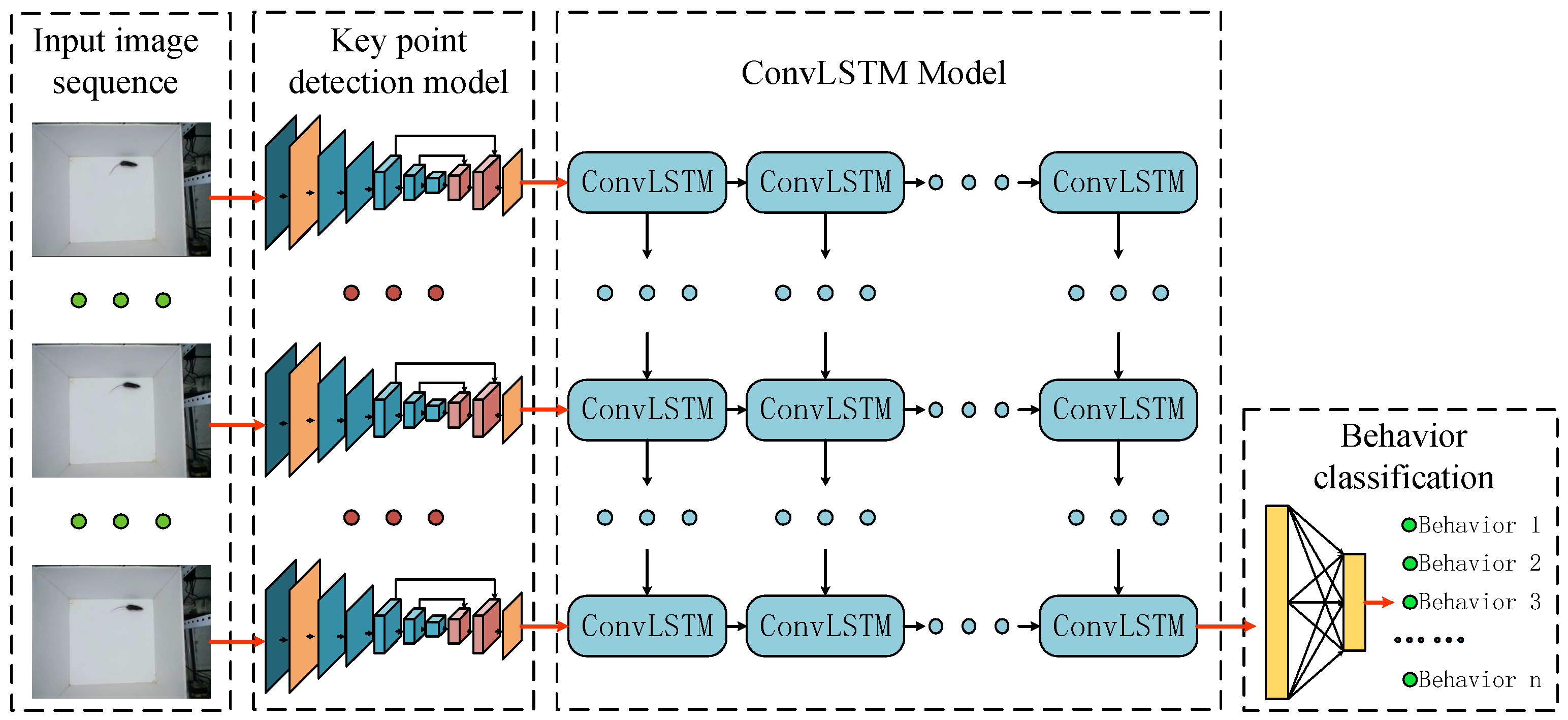
2.1. Structure of Algorithm

This study included the construction of a murine motion behavior recognition model based on the fusion of a keypoint detection algorithm and a ConvLSTM network. The model’s structure is shown in Figure 1. First, the keypoints of the nose, left ear, right ear, and tail root of the mouse were detected by the improved DeepLabCut algorithm. The keypoint feature map sequences of adjacent images were then input into the ConvLSTM network to extract the spatiotemporal information of behavioral changes. Finally, the five behaviors of the mice were classified as walking straight, resting, grooming, standing upright, and turning. Based on the keypoint detection and behavior classification results, the movement and behavior indicators in the murine behavioral experiments can be calculated. These include motion speed, angular speed, trajectory, and frequency and time of behavior.

2.2. Improved DeepLabCut Network

DeepLabCut is an open-source system for single-target pose estimation. Based on transfer learning, it can accurately detect keypoints without large quantities of training data, and has been tested and calibrated across species of mice, flies, and humans. The structure of the algorithm is shown in Figure 2. Its backbone network is Resnet50, which has been pre-trained in ImageNet [25]—a large target-recognition image database—eliminating the need for a large number of training samples. Unlike the standard Resnet50 network, DeepLabCut limits the downsampling multiple of the Resnet50 network to 16 times in order to obtain a larger feature map size. Specifically, the positions of Block2, Block3, and Block4 in Figure 2 are not downsampled, and Block represents the residual block in Resnet50.

DeepLabCut uses a heatmap plus coordinate offset to predict keypoint locations. The Resnet50 network outputs a feature map of 2048 channels and, by transpose convolution, obtains the class probability feature map with the number of channels as the number of keypoints, as well as the coordinate offset feature map, where the number of channels is twice the number of keypoints. The coordinate offset provides more accurate location information than the traditional method of using only a heatmap for prediction. Therefore, DeepLabCut needs two parts of the loss function during training: for the category probability part, the binary cross-entropy loss is used, and for the coordinate offset part, the Huber loss is used. The loss function formula is as follows:

$$los{s}_{sigmoid\_cross\_entropy}=y_c\ast -\log \left(\frac{1}{1+e^{-x_c}}\right)-\log \left(\frac{e^{-x_c}}{1+e^{-x_c}}\right)\ast \left(1-y_c\right)$$

$$=x_c-x_c\ast y_c+\log \left(1+e^{-x_c}\right)$$

(1)

$$los{s}_{huber}=\{\begin{array}{c}\frac{1}{2}{\left(y_r-x_r\right)}^2 for \left|y_r-x_r\right|\le \delta \\ \delta \left|y_r-x_r\right|-\frac{1}{2}{\delta }^2 otherwise\end{array}$$

(2)

$$los{s}_{all}=los{s}_{sigmoid\_cross\_entropy}+los{s}_{huber}$$

(3)

where $y_c$ is the category label, $y_r$ is the real coordinate offset, $x_c$ is the predicted category probability, $x_r$ is the predicted coordinate offset, and $\delta$ is a hyperparameter used to judge whether a point is a singular data point. When the predicted deviation is less than $\delta$, the mean square error (MSE) is adopted; when the predicted error is greater than $\delta$, the linear error is adopted to prevent oversensitivity to outliers.

In keypoint detection tasks, large receptive fields and multiscale information are crucial. First, the representation of different keypoints may require information at different scales. Second, large receptive fields and multiscale information can implicitly establish spatial connections between keypoints. The convolutional pose machine (CPM) [26] and stacked hourglass network (Hourglass) [27] algorithms use cascade networks to obtain large receptive fields and multiscale information. To make the keypoint detection model suitable for most murine behavioral scenarios, this study used atrous spatial pyramid pooling (ASPP) in DeepLabV3 [28] to fuse context information at multiple scales. Specifically, the intermediate convolution kernel of the residual unit in the residual block was replaced by the ASPP module, as shown in Figure 3. The ASPP module consisted of one 1 × 1 convolution, three 3 × 3 dilated convolutions with different expansion rates, and a global average pooling, and finally used the concatenation operation to fuse multiscale features. In this paper, the effect of the ASPP module was verified by the ablation experiment, and the effects of different sites and different expansion rates on the model were compared. In the following sections, DLC_b1_r1 means that the ASPP module has been inserted into Block1, and the expansion rates are 1, 2, and 4; DLC_b12_r2 means that the ASPP module has been inserted into Block1 and Block2, and the expansion rates are 2, 4, and 6.

The keypoint network plays two roles in this study: The first is to output precise coordinates of the keypoints of the mouse’s nose, left ear, right ear, and tail root. The second is to output a feature map containing the spatial posture information of the mice, which is combined with context information to recognize murine behavior.

2.3. Convolutional Long Short-Term Memory Network

Behavior can be described as posture change over time. Traditional behavior recognition algorithms extract distance and angle features between keypoints and then use a long short-term memory (LSTM) [29] model to represent the temporal relationships between behaviors, as proposed by Fu et al. [20]. However, do the obtained features comprehensively summarize the spatial connections between keypoints? Do they properly represent the temporal change in posture? How should false and missing results in the keypoint detection model be dealt with? Artificial features must address these considerations.

This paper introduces the ConvLSTM [30] to solve the above problem. ConvLSTM replaces the fully connected layer in FC-LSTM with a convolution, which can capture spatial features in multidimensional data. The information transmission mode is shown in Equation (4). The state of the previous moment can be transmitted to the next moment in a spatial form, so that spatiotemporal features can be extracted:

$$i_t=\sigma \left(W_{xi}\ast X_t+W_{hi}\ast h_{t-1}+b_i\right)$$

$$f_t=\sigma \left(W_{xf}\ast X_t+W_{hf}\ast h_{t-1}+b_f\right)$$

$$C_t=f_t\circ C_{t-1}+i_t\circ \tan \mathrm{h}\left(W_{xc}\ast X_t+W_{hc}\ast h_{t-1}+b_c\right)$$

(4)

$$o_t=\sigma \left(W_{xo}\ast X_t+W_{ho}\ast h_{t-1}+b_o\right)$$

$$h_t=o_t\circ \tan \mathrm{h}\left(C_t\right)$$

where $i_t$, $f_t$, and $o_t$ are the input, forget, and output gates, respectively, with step size t, $X_t$ represents the input data, $C_t$ is the storage cell state, $h_t$ is the output of the network at time t, “*” represents the convolution operation, and “∘” is the Hadamard product.

In the murine behavior recognition task, the sequence of adjacent frames’ feature maps, which is output by the keypoint detection algorithm, was used as input to the ConvLSTM network to model dynamic changes in behavior. The structure of the ConvLSTM network is shown in Figure 4, and its main functions are as follows: First, the keypoint feature maps reduce redundant information in the images. Second, the keypoints contain not only the spatial connections between keypoints, but also location information for the mice. For example, the position and spatial relationship of keypoints did not change during static behavior, but the location and spatial relationship of keypoints changed simultaneously as the mouse moved. Third, behavior is jointly determined by previous and current actions; therefore, the keypoint feature maps of previous and current frames are used as inputs to jointly determine current behavior, which is consistent with the definition of behavior. Fourth, it does not require additional artificial design features—the network can implicitly model the temporal relations of keypoints when behavior occurs, and even if there are false and missing results, it can be used as a representation of behavior.

Specifically, four ConvLSTM layers were used to extract spatiotemporal information; the numbers of convolution kernels were 256, 128, 64, and 5, respectively, and the size of the convolution kernels was 3 × 3. Global average pooling was then used to achieve behavior classification. The resolution of the feature maps output by each layer remained unchanged, which is more conducive to learning spatial information. The structure of the ConvLSTM network is shown in Figure 4.

3. Experiments and Results

3.1. Dataset

In this study, a dataset containing four keypoints representing the mouse’s nose, left ear, right ear, and tail root was produced, which was taken from the top in an open-field experimental box, with an image resolution of 640 × 480. The video was shot in a dark room using the same device, using fill lights to fix the light intensity at 200 lux. In total, 24 videos were captured, each of which was 5 min long and featured two mice. The videos were shot at different heights and with different background colors. The dataset comprehensively considered the influence of behavior, color, and scale on model performance. It included five behaviors (walking straight, resting, grooming, standing upright, and turning), four background colors (white, light gray, dark gray, and black), and three shooting heights (60, 70, and 80 cm). Figure 5 shows images from the dataset. There were 2700 images in the training set—including only the scale of 70 cm, with a uniform distribution of colors—and 1200 images in the test set, with uniform distribution of colors and scales. Each image was split from the videos above and randomly assigned to the training set or test set.

For the behavior recognition task, to ensure consistency of spatial scale, the videos were collected at a height of 70 cm. The behavior recognition dataset contained five types of behaviors: walking straight, resting, grooming, standing upright, and turning. Each type of behavior was represented by 600 labeled images, of which 75% were randomly selected as the training set and 25% as the test set. All stages of a given behavior were covered as much as possible in the labeling process. During training and testing, an image sequence consisting of the annotated frame and several frames preceding the annotated frame was used as an input to the model. Figure 6 shows an example of an image sequence of the five types of behaviors, in which the sequence length is five and the interval between frames is two.

3.2. Evaluation Metrics

In this study, the percentage of correct keypoints (PCK) was used as the evaluation metric for keypoint detection. The PCK refers to the proportion of the normalized distances between the detected keypoints and their corresponding labels that is less than a set threshold. In the FLIC dataset [31], the torso size was used as the scale factor to calculate the normalized distance, while in the MPII dataset [32], the length of the head was used as the scale factor. The calculation formula of the PCK is as follows:

$$PC{K}_i^k=\frac{{{\displaystyle \sum }}_p\delta (\frac{d_{pi}}{d_p^{def}}\le T_k)}{{{\displaystyle \sum }}_{p}1}, \delta \left(r\right)=\{\begin{array}{c}1 if r=True \\ 0 if r=False\end{array}$$

(5)

$$PC{K}_{mean}^k=\frac{{{\displaystyle \sum }}_p{{\displaystyle \sum }}_i\delta (\frac{d_{pi}}{d_p^{def}}\le T_k)}{{{\displaystyle \sum }}_p{{\displaystyle \sum }}_{i}1}, \delta \left(r\right)=\{\begin{array}{c}1 if r=True \\ 0 if r=False\end{array}$$

(6)

where $i$ represents the particular keypoint, $k$ is the threshold, $p$ is the image, $d_{pi}$ is the Euclidean distance between the predicted and true values of keypoint $i$ in the $p$th image, $d_p^{def}$ is the scale factor of the pth image, $PC{K}_i^k$ represents the PCK for the keypoint of category $i$ under threshold $T_k$, and $PC{K}_{mean}^k$ represents the average PCK for all keypoints under threshold $T_k$. In this study, the distance between the ears in each frame was denoted by $d_p^{def}$. If the distance between the ears could not be calculated, the median of the scale could be used as the scale factor—60 cm was 15.29, 70 cm was 12.85, and 80 cm was 10.81. $T_k\in \left[0,0.1,0.2,0.3,0.4\right]$.

For the behavior recognition task, the accuracy and the confusion matrix were used as evaluation metrics. Accuracy was defined as the ratio of samples that were predicted correctly to the total number of samples considered. Each column of the confusion matrix represented the category of prediction, and the total number of items in each column represented the number of data items predicted for the relevant category. Each row represented the true category, and the total number of items in each row represented the number of data instances in that category.

3.3. Experimental Details

In the keypoint detection task, CPM [26], Hourglass [27], DeepLabCut, and the improved DeepLabCut were used for comparison. CPM used six stage units and trained for 300 epochs. Stacked hourglass used four hourglass modules and trained for 1000 epochs, with a learning rate of 0.0001. CPM and stacked hourglass needed to crop out the mouse in the original image for detection and then map the coordinates back to the original image. DeepLabCut and the improved DeepLabCut required a total of 1,030,000 iterations. The learning rate was 0.005 for the first 10,000 iterations, 0.02 for 10,000 to 430,000, 0.002 for 430,000 to 730,000, and 0.001 for the final stage, using Resnet50 weights pre-trained on ImageNet.

In the murine behavior recognition task, 3DCNN [33,34], LSTM, and Bi-LSTM [35,36] were compared with ConvLSTM. The 3DCNN network also used the keypoint feature map sequence as an input. This study used a four-layer 3D convolution; the numbers of convolution kernels were 64, 64, 128, and 256, respectively, and the size of the convolution kernel was 3 × 3 × 3. The 3DCNN network used the full connection and softmax functions for classification, and trained for a total of 10 epochs. Eleven features were extracted from the murine keypoints for training LSTM and Bi-LSTM, as shown in Figure 7. The LSTM network consisted of four layers with 64, 64, 128, and 256 neurons, respectively, used full connections for classification, and trained for a total of 50 epochs. The bi-LSTM network’s training parameters were the same as those for LSTM, except that Bi-LSTM utilized the information in the later frames.

3.4. Results

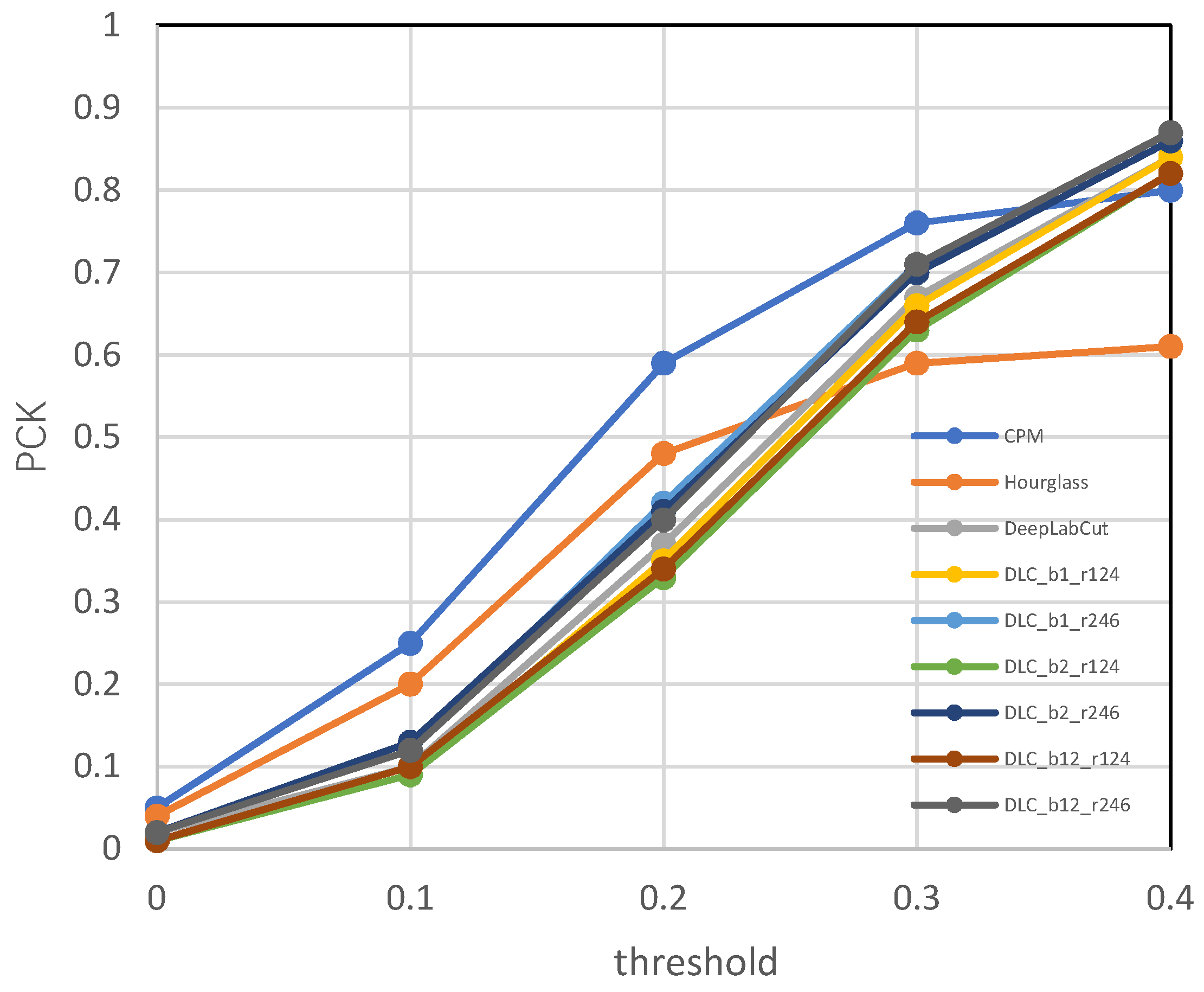
3.4.1. Results of Keypoint Detection

Table 1. Comparison of algorithms between different keypoints and different scales (PCK).

Method	Keypoints				Heights			Avg	FPS
	Nose	Left Ear	Right Ear	Tail Root	60 cm	70 cm	80 cm
CPM	$0.76\pm 0.01$	$0.79\pm 0.02$	$0.85\pm 0.02$	$0.80\pm 0.01$	$0.88\pm 0.02$	$0.84\pm 0.02$	$0.69\pm 0.03$	$0.80\pm 0.01$	15.1
Hourglass	$0.59\pm 0.04$	$0.65\pm 0.04$	$0.71\pm 0.02$	$0.50\pm 0.02$	$0.72\pm 0.02$	$0.67\pm 0.03$	$0.44\pm 0.05$	$0.61\pm 0.02$	14.5
DeepLabCut	$0.84\pm 0.03$	$0.85\pm 0.01$	$0.87\pm 0.02$	$0.81\pm 0.02$	$0.94\pm 0.04$	$0.91\pm 0.04$	$0.68\pm 0.01$	$0.84\pm 0.01$	18.4
DLC_b1_r1	$0.85\pm 0.05$	$0.85\pm 0.02$	$0.85\pm 0.01$	$0.84\pm 0.01$	$0.92\pm 0.02$	$0.92\pm 0.01$	$0.69\pm 0.04$	$0.85\pm 0.01$	17.5
DLC_b1_r2	$0.88\pm 0.01$	$0.88\pm 0.02$	$0.91\pm 0.02$	$0.82\pm 0.02$	$0.92\pm 0.03$	$0.92\pm 0.02$	$0.77\pm 0.04$	$0.87\pm 0.01$	16.7
DLC_b2_r1	$0.83\pm 0.02$	$0.81\pm 0.02$	$0.84\pm 0.02$	$0.81\pm 0.04$	$0.92\pm 0.02$	$0.91\pm 0.01$	$0.64\pm 0.03$	$0.82\pm 0.02$	16.9
DLC_b2_r2	$0.87\pm 0.01$	$0.86\pm 0.02$	$0.87\pm 0.03$	$0.83\pm 0.01$	$0.94\pm 0.03$	$0.92\pm 0.03$	$0.71\pm 0.04$	$0.85\pm 0.01$	17.2
DLC_b12_r1	$0.84\pm 0.03$	$0.83\pm 0.03$	$0.82\pm 0.02$	$0.80\pm 0.02$	$0.91\pm 0.02$	$0.91\pm 0.02$	$0.65\pm 0.01$	$0.82\pm 0.01$	15.4
DLC_b12_r2	$0.87\pm 0.02$	$0.88\pm 0.01$	$0.91\pm 0.01$	$0.83\pm 0.03$	$0.92\pm 0.01$	$0.92\pm 0.03$	$0.79\pm 0.03$	$0.87\pm 0.01$	14.6

shows the results of a performance comparison between different keypoint detection algorithms, with a threshold of 0.4. As can be seen from Table 1, among CPM, Hourglass, and DeepLabCut, the accuracy of DeepLabCut for each keypoint was the highest, and the detection speed was 18.4 frames per second. After the ASPP module was added, DLC_b1_r2, DLC_b2_r2, and DLC_b12_r2 achieved high accuracy on each keypoint, and the PCK increased by 2–3%, proving that the ASPP module can indeed improve keypoint detection accuracy under a high expansion rate. At the same time, the results at different scales show that this improvement in accuracy was related to the improved accuracy of small-scale target detection, with the PCK at 80 cm increasing from 68% to 77%. However, the location where ASPP joined had little effect, but one bias was that when the ASPP module was located in the shallow layers of the network, the accuracy rate was higher. The reason for this may be that the shallow layer of the network contains detailed features, the deep layer has semantic features, and the keypoints at different scales have different detailed features rather than semantic information. The addition of the ASPP module incurred extra calculation, and the FPS decreased, but this decline was acceptable. Considering the amount of computation, DLC_b1_r2 was selected as the optimal model in this paper.

The parameters were consistent during training, but the order of images was shuffled. Each algorithm was trained 10 times; the results are reported as mean differences at a 95% confidence interval. For detailed results, see the Data Availability Statement. “Keypoints” represents the PCK of each algorithm at different keypoints; “Heights” represents the PCK of each algorithm at different scales; “Avg” represents the average PCK of different keypoints.

Figure 8 compares the performance of each algorithm under different thresholds. The smaller the threshold, the smaller the prediction error. Although the DeepLabCut series algorithms achieved high PCK when the threshold was 0.4, their performance was worse than that of the CPM and stacked hourglass algorithms at a lower threshold. The reasons for this may be as follows: First, the CPM and stacked hourglass algorithms both use intermediate supervision, making location information more accurate in continuous multistage learning. Second, the CPM and stacked hourglass algorithms both use the method of cropping out the mouse region before detection, whereas the DeepLabCut series directly detects on the original image. Analysis of the series of improvements in DeepLabCut shows that the ASPP module with a high expansion rate not only improves prediction accuracy, but also reduces prediction error.

3.4.2. Results of Behavior Recognition

Table 2. Behavior recognition accuracy under different time scales.

Sequence Length	Sequence Interval	Resting	Grooming	Standing Upright	Walking Straight	Tuning	Avg
6	0	$0.72\pm 0.03$	$0.99\pm 0.01$	$0.95\pm 0.01$	$0.99\pm 0.01$	$0.91\pm 0.02$	$0.91\pm 0.01$
	1	$0.56\pm 0.05$	$0.99\pm 0.01$	$0.95\pm 0.00$	$0.99\pm 0.01$	$0.92\pm 0.02$	$0.86\pm 0.01$
	2	$0.63\pm 0.01$	$0.97\pm 0.02$	$0.93\pm 0.03$	$0.98\pm 0.02$	$0.91\pm 0.02$	$0.88\pm 0.01$
7	0	$0.78\pm 0.03$	$0.99\pm 0.01$	$0.95\pm 0.02$	$1.00\pm 0.00$	$0.97\pm 0.02$	$0.93\pm 0.01$
	1	$0.70\pm 0.02$	$0.97\pm 0.01$	$0.95\pm 0.02$	$0.98\pm 0.01$	$0.92\pm 0.02$	$0.90\pm 0.01$
	2	$0.77\pm 0.01$	$0.97\pm 0.02$	$0.90\pm 0.04$	$0.99\pm 0.01$	$0.94\pm 0.03$	$0.91\pm 0.02$
8	0	$0.72\pm 0.03$	$0.98\pm 0.01$	$0.93\pm 0.02$	$0.99\pm 0.01$	$0.94\pm 0.03$	$0.91\pm 0.01$
	1	$0.55\pm 0.06$	$0.97\pm 0.02$	$0.91\pm 0.02$	$0.97\pm 0.02$	$0.97\pm 0.01$	$0.86\pm 0.02$
	2	$0.78\pm 0.04$	$0.94\pm 0.02$	$0.92\pm 0.02$	$0.96\pm 0.02$	$0.94\pm 0.02$	$0.90\pm 0.01$

Each algorithm was trained 10 times; the results are reported as mean differences at a 95% confidence interval. “Sequence length” represents the length of the continuous image sequence; “Sequence interval” represents the interval between adjacent frames in a continuous image sequence; “Avg” represents the average accuracy of different behaviors.

shows the accuracy of each behavior under different input parameters. Clearly, the accuracy of different behaviors varied greatly. The accuracy of resting behavior was the lowest, at less than 80%; the accuracies for grooming and walking straight were the highest, at greater than 95%. Second, the recognition rate varied greatly with different input parameters. For example, for resting behaviors, when the sequence interval was 1, the accuracy was the lowest, but for most behaviors, the influence of the input parameters did not adhere to obvious rules. Analyzing the input data leads to the conclusion that the time scales of different behaviors—or even the same behaviors—are not always the same, and that changes in input parameters lead to different information being received by the network. When information is redundant or lacking, it is difficult to form a consistent understanding of behaviors. Because the objective law of different scales exhibited by behavior cannot be changed, the key is to enable the network to adapt to different time scales, which will be the focus of upcoming research. The results presented here demonstrate the feasibility of ConvLSTM for behavior recognition. This network had the highest accuracy of $0.93\pm 0.01$ when the length of the sequence was seven and the sequence interval was zero.

Table 3. Behavior recognition accuracy of different algorithms.

Method	Resting	Grooming	Standing Upright	Walking Straight	Turning	Avg
LSTM	$0.72\pm 0.02$	$0.97\pm 0.02$	$0.98\pm 0.01$	$0.91\pm 0.02$	$0.95\pm 0.01$	$0.95\pm 0.01$
Bi-LSTM	$0.75\pm 0.04$	$0.99\pm 0.01$	$0.97\pm 0.02$	$0.98\pm 0.01$	$0.98\pm 0.01$	$0.92\pm 0.01$
3DCNN	$0.60\pm 0.02$	$0.92\pm 0.02$	$0.85\pm 0.03$	$0.96\pm 0.02$	$0.99\pm 0.01$	$0.83\pm 0.02$
ConvLSTM	$0.78\pm 0.03$	$0.99\pm 0.01$	$0.95\pm 0.02$	$1.00\pm 0.00$	$0.97\pm 0.02$	$0.93\pm 0.01$

Each algorithm was trained 10 times, and the results are reported as mean differences at a 95% confidence interval. “Avg” indicates the average accuracy of different behaviors.

compares the recognition accuracy of different algorithms. It is apparent that the algorithms of the long short-term memory network series—such as LSTM, Bi-LSTM, and ConvLSTM—had higher accuracy than 3DCNN. Although 3DCNN can also process time series, its output is only related to the input—not to the order of the input. Thus, it could not handle the time series. Compared with the one-dimensional LSTM network, ConvLSTM achieved the highest accuracy of $0.93\pm 0.01$, indicating that the implicit establishment of spatial temporal information is more conducive to the network’s understanding of behavior. Finally, compared with LSTM, the accuracy of Bi-LSTM was increased by 2.2%, indicating that the context information in the video sequence helped in recognizing behavior. This provides inspiration for the next step to improve the ConvLSTM network. A comparison of behaviors showed that the accuracy of the method in identifying resting was significantly lower than that in identifying the other behaviors. We generated a confusion matrix to analyze identifications by each algorithm to explore the reasons for the low accuracy in identifying resting behavior, as shown in Figure 9.

It is apparent that the misrecognition of behaviors by different algorithms was similar. For resting and grooming behaviors, the misrecognition rate was high because, in both behaviors, the mouse is generally immobile; although the keypoints fluctuate over a small range in the grooming behavior, this jitter was reflected in the keypoint feature map with little difference, where this resulted in similar spatial distribution of keypoint feature maps. Therefore, it is difficult for the network to distinguish between resting and grooming behaviors. On the other hand, the misrecognition rates of upright and turning behavior were also high, because upright behavior often contains turning behavior. In summary, this study reveals the complexity of behavior recognition, which cannot be simply recognized directly through the network. One possible method is to decompose behavior into behavioral elements that are easily recognized by the algorithm, and then to infer behavior according to the combination of behavioral elements.

4. Discussion

We integrated the DeepLabCut algorithm with the ASPP module to detect the nose, left ear, right ear, and tail root of mice, and achieved a PCK of 0.87 ± 0.01. Compared with the original DeepLabCut, the overall performance improved by 3%. The performance improved by 9% for small targets (shooting height at 80 cm). This shows that ASPP can fuse multiscale information and enable the network to adapt to changes in the scale of the object. The closer the ASPP module was to the shallow layer, and the higher the expansion rate, the better the performance of the proposed method. The network delivered optimal performance when the ASPP module was at Block1 and the expansion rates were 2, 4, and 6. This result was possibly obtained because the shallow layers of the network contain more detailed information on objects, and the receptive field was smaller. The shallow features were different for the representation of objects at different scales. The semantic information tended to be consistent for deep layers of the network. As a result, the ASPP module worked well at the shallow level. A higher expansion rate may be applicable to the dataset in this paper. The optimal parameters of the expansion rate may be different for different detection tasks, and this requires more detailed research. In addition, we found that when highly precise identification was required, the accuracy of the DeepLabCut series algorithms was not as high as that of CPM and Hourglass, because of their low input resolution. Finding ways to make use of finer local information will be the focus of our next improvement to this algorithm.

The traditional analysis of the behavior of mice has focused only on the parameters of their movement or posture [37,38,39,40,41], and has paid little attention to their behavior. We propose an algorithm that integrates a keypoint detection model with the ConvLSTM network to detect the motion behavior of mice. This algorithm achieved an average accuracy of 93.8% in identifying the five behaviors of walking straight, resting, grooming, standing upright, and turning, where this was higher than the accuracies of the LSTM, Bi-LSTM, and 3DCNN. Behavior can be expressed as a pattern of spatiotemporal changes in posture. The map of keypoint features containing posture-related information was used as the input to the ConvLSTM network to implicitly establish the relationships between keypoints. The ConvLSTM network passed the state information of the previous moment to the next moment. This is consistent with the definition of behavior. The output of ConvLSTM network thus contained temporal and spatial information on behavioral changes. We experimentally demonstrated the feasibility of this method, and explored the impact of behavioral factors at the temporal scale on network performance. The durations for which different behaviors could be sustained were different, but the length of the sequence of the network input was fixed, and led to varying network performance at different time scales. Although we experimentally determined the optimal parameters of the time scale parameters, the network did not have the ability to adapt to different time scales of behavior. In addition, ConvLSTM could not distinguish between similar behaviors, such as resting and grooming. One possible solution to this is to decompose behaviors into behavioral elements that are easily identifiable by the algorithm, and then to combine different behavioral elements into behaviors [42,43].

We can use DeepLabCut and the ConvLSTM network to detect both the parameters of motion and the behavior of mice. For example, we can use keypoints to calculate the speed of movement of a mouse, draw a trajectory map, and determine the difference between its central and peripheral movements. The results of behavior recognition of each frame can then be used to calculate the frequency and duration of each behavior. We provide an accurate and quantitative tool for behavioral analysis that is important for reducing the workload of researchers and objectively analyzing experimental data. However, the proposed algorithm still has many limitations. For example, the FPS of the improved DeepLabCut was reduced from 18.4 to 16.7 due to the addition of the ASPP module. Although this still satisfies the requirements of use, this limitation renders it unsuitable for some scenarios requiring real-time detection. In addition, the proposed algorithm requires training two models, which is cumbersome. Implementing an end-to-end model will also be the focus of our future research in this area.

5. Conclusions

In this study, we proposed a method to identify the motion behavior of mice based on the DeepLabCut model and the ConvLSTM network. The results of our experiments showed that the ASPP module can improve the multiscale representation capability of the network. The average PCK of DeepLabCut increased from 84% to 87% after the ASPP module was added, and the accuracy of the method at detecting small targets increased by 9%. The performance of the network was better when the ASPP module was located in the shallow layer of the network. We also demonstrated ConvLSTM’s ability to extract temporal and spatial information from keypoint feature maps, and used it for behavior classification. Moreover, we verified the effect of the temporal scale of behavior on the performance of the model. When the length of the sequence was seven and the sequence interval was zero, the proposed method delivered the best performance, with an average accuracy of 93.8%, which was higher than those of the LSTM, Bi-LSTM, and 3DCNN.

References

1. Jin, W.L. Application of ethology to modern life science research. Lab. Anim. Comp. Med. 2008, 28, 1–3. [Google Scholar] [CrossRef]
2. Xu, K. Outline of Neurobiology; Science Press: Beijing, China, 2001; pp. 1–15. ISBN 7030073975. [Google Scholar]
3. Fernandez-Gonzalez, R.; Moreira, P.; Bilbao, A.; Jimenez, A.; Perez-Crespo, M. Long-term effect of in vitro culture of mouse embryos with serum on mRNA expression of imprinting genes, development, and behavior. Proc. Natl. Acad. Sci. USA 2004, 101, 5880–5885. [Google Scholar] [CrossRef] [PubMed] [Green Version]
4. Zhang, S.; Yuan, S.; Huang, L.; Zheng, X.; Wu, Z.; Xu, K.; Pan, G. Human Mind Control of Rat Cyborg’s Continuous Locomotion with Wireless Brain-to-Brain Interface. Sci. Rep. 2019, 9, 1321. [Google Scholar] [CrossRef] [PubMed]
5. May, C.H.; Sing, H.C.; Cephus, R.; Vogel, S.; Shaya, E.K.; Wagner, H.N. A new method of monitoring motor activity in baboons. Behav. Res. Methods Instrum. Comput. 1996, 28, 23–26. [Google Scholar] [CrossRef] [Green Version]
6. Weerd, H.; Bulthuis, R.; Bergman, A.; Schlingmann, F.; Zutphen, L. Validation of a new system for the automatic registration of behaviour in mice and rats. Behav. Process. 2001, 53, 11–20. [Google Scholar] [CrossRef]
7. Osechas, O.; Thiele, J.; Bitsch, J.; Wehrle, K. Ratpack: Wearable sensor networks for animal observation. In Proceedings of the International Conference of the IEEE Engineering in Medicine & Biology Society, Vancouver, BC, Canada, 20–25 August 2008. [Google Scholar] [CrossRef]
8. Heeren, D.J.; Cools, A.R. Classifying postures of freely moving rodents with the help of fourier descriptors and a neural network. Behav. Res. Methods Instrum. Comput. 2000, 32, 56–62. [Google Scholar] [CrossRef] [Green Version]
9. Zhang, M. Study and Application of Animal Behavior Automatic Analysis Based on Posture Recognition; Zhejiang University: Hangzhou, China, 2005. [Google Scholar]
10. Alexander, M.; Pranav, M.; Cury, K.M.; Taiga, A.; Murthy, V.N.; Weygandt, M.M.; Matthias, B. DeepLabCut: Markerless pose estimation of user-defined body parts with deep learning. Nat. Neurosci. 2018, 21, 1281–1290. [Google Scholar] [CrossRef]
11. Nguyen, N.G.; Phan, D.; Lumbanraja, F.R.; Faisal, M.R.; Satou, K. Applying Deep Learning Models to Mouse Behavior Recognition. J. Biomed. Sci. Eng. 2019, 12, 183–196. [Google Scholar] [CrossRef] [Green Version]
12. Carreira, J.; Zisserman, A. Quo Vadis, Action Recognition? A New Model and the Kinetics Dataset. In Proceedings of the 2017 IEEE Conference on Computer Vision and Pattern Recognition (CVPR), Honolulu, HI, USA, 21–26 July 2017. [Google Scholar]
13. Du, T.; Wang, H.; Torresani, L.; Ray, J.; Lecun, Y. A Closer Look at Spatiotemporal Convolutions for Action Recognition. In Proceedings of the 31st IEEE/CVF Conference on Computer Vision and Pattern Recognition (CVPR), Salt Lake City, UT, USA, 18–23 June 2018. [Google Scholar] [CrossRef] [Green Version]
14. Liu, D.; Li, W.; Ma, C.; Zheng, W.; Yao, Y.; Tso, C.F.; Zhong, P.; Chen, X.; Song, J.H.; Choi, W.; et al. A common hub for sleep and motor control in the substantia nigra. Science 2020, 367, 440–448. [Google Scholar] [CrossRef]
15. Milletari, F.; Navab, N.; Ahmadi, S.A. V-Net: Fully Convolutional Neural Networks for Volumetric Medical Image Segmentation. In Proceedings of the 4th IEEE International Conference on 3D Vision (3DV), Stanford, CA, USA, 25–28 October 2016. [Google Scholar] [CrossRef] [Green Version]
16. He, K.; Zhang, X.; Ren, S.; Sun, J. Deep Residual Learning for Image Recognition. In Proceedings of the 2016 IEEE Conference on Computer Vision and Pattern Recognition (CVPR), Las Vegas, NV, USA, 27–30 June 2016. [Google Scholar] [CrossRef] [Green Version]
17. Ren, S.; He, K.; Girshick, R.; Sun, J. Faster R-CNN: Towards Real-Time Object Detection with Region Proposal Networks. IEEE Trans. Pattern Anal. Mach. Intell. 2017, 39, 1137–1149. [Google Scholar] [CrossRef] [Green Version]
18. He, K.; Gkioxari, G.; Dollár, P.; Girshick, R. Mask R-CNN. IEEE Trans. Pattern Anal. Mach. Intell. 2017, 40, 386–397. [Google Scholar] [CrossRef]
19. Wang, H.; Kläser, A.; Schmid, C.; Liu, C.-L. Dense trajectories and motion boundary descriptors for action recognition. Int. J. Comput. Vis. 2013, 103, 60–79. [Google Scholar] [CrossRef] [Green Version]
20. Fu, Z.R.; Wu, S.X.; Wu, X.Y. Human Action Recognition Using BI-LSTM Network Based on Spatial Features. J. East China Univ. Sci. Technol. 2021, 47, 225–232. [Google Scholar] [CrossRef]
21. Lu, X.; Chia-Chih, C.; Aggarwal, J.K. View invariant human action recognition using histograms of 3D joints. In Proceedings of the 2012 IEEE Computer Society Conference on Computer Vision and Pattern Recognition Workshops (CVPR Workshops), Providence, RI, USA, 16–21 June 2012. [Google Scholar] [CrossRef]
22. Yan, S.; Xiong, Y.; Lin, D. Spatial temporal graph convolutional networks for skeleton-based action recognition. In Proceedings of the Thirty-Second AAAI Conference on Artificial Intelligence, New Orleans, LA, USA, 2–7 February 2018. [Google Scholar]
23. Shahroudy, A.; Liu, J.; Ng, T.-T.; Wang, G. NTU RGB plus D: A Large Scale Dataset for 3D Human Activity Analysis. In Proceedings of the 2016 IEEE Conference on Computer Vision and Pattern Recognition (CVPR), Seattle, WA, USA, 27–30 June 2016; pp. 1010–1019. [Google Scholar] [CrossRef] [Green Version]
24. Song, S.; Lan, C.; Xing, J. An end-to-end spatiotemporal attention model for human action recognition from skeleton data. arXiv 2016, arXiv:1611.06067. [Google Scholar] [CrossRef]
25. Deng, J.; Dong, W.; Socher, R.; Li, L.J.; Li, F.F. ImageNet: A Large-Scale Hierarchical Image Database. In Proceedings of the 2009 IEEE Computer Society Conference on Computer Vision and Pattern Recognition (CVPR 2009), Miami, FL, USA, 20–25 June 2009. [Google Scholar] [CrossRef] [Green Version]
26. Wei, S.E.; Ramakrishna, V.; Kanade, T.; Sheikh, Y. Convolutional Pose Machines. In Proceedings of the 2016 IEEE Conference on Computer Vision and Pattern Recognition (CVPR), Seattle, WA, USA, 27–30 June 2016. [Google Scholar] [CrossRef] [Green Version]
27. Newell, A.; Yang, K.U.; Deng, J. Stacked Hourglass Networks for Human Pose Estimation. In Proceedings of the 14th European Conference on Computer Vision (ECCV), Amsterdam, The Netherlands, 8–16 October 2016; pp. 483–499. [Google Scholar] [CrossRef] [Green Version]
28. Chen, L.C.; Papandreou, G.; Schroff, F.; Adam, H. Rethinking Atrous Convolution for Semantic Image Segmentation. arXiv 2017, arXiv:1706.05587. [Google Scholar] [CrossRef]
29. Hochreiter, S.; Schmidhuber, J. Long Short-Term Memory. Neural Comput. 1997, 9, 1735–1780. [Google Scholar] [CrossRef]
30. Shi, X.; Chen, Z.; Wang, H.; Yeung, D.Y.; Wong, W.K.; Woo, W.C. Convolutional LSTM Network: A Machine Learning Approach for Precipitation Nowcasting. In Proceedings of the 29th Annual Conference on Neural Information Processing Systems (NIPS), Montreal, QC, Canada, 7–12 December 2015. [Google Scholar]
31. Hashimoto, T.; Izawa, Y.; Yokoyama, H.; Kato, T.; Moriizumi, T. A new video/computer method to measure the amount of overall movement in experimental animals (two-dimensional object-difference method). J. Neurosci. Methods 1999, 91, 115–122. [Google Scholar] [CrossRef]
32. Andriluka, M.; Pishchulin, L.; Gehler, P.; Schiele, B. 2D Human Pose Estimation: New Benchmark and State of the Art Analysis. In Proceedings of the 27th IEEE Conference on Computer Vision and Pattern Recognition (CVPR), Columbus, OH, USA, 23–28 June 2014. [Google Scholar] [CrossRef]
33. Ji, S.; Xu, W.; Yang, M.; Yu, K. 3D Convolutional Neural Networks for Human Action Recognition. IEEE Trans. Pattern Anal. Mach. Intell. 2013, 35, 221–231. [Google Scholar] [CrossRef] [Green Version]
34. Jiang, H.; Pan, Y.; Zhang, J.; Yang, H. Battlefield Target Aggregation Behavior Recognition Model Based on Multi-Scale Feature Fusion. Symmetry 2019, 11, 761. [Google Scholar] [CrossRef] [Green Version]
35. Zhu, M.K.; Lu, X.L. Human Action Recognition Algorithm Based on Bi-LSTMAttention Model. Laser Optoelectron. Prog. 2019, 56, 9. [Google Scholar] [CrossRef]
36. Park, S.; On, B.W.; Lee, R.; Park, M.W.; Lee, S.H. A Bi–LSTM and k-NN Based Method for Detecting Major Time Zones of Overloaded Vehicles. Symmetry 2019, 11, 1160. [Google Scholar] [CrossRef] [Green Version]
37. Risse, B.; Mangan, M.; Webb, B.; Pero, L.D. Visual Tracking of Small Animals in Cluttered Natural Environments Using a Freely Moving Camera. In Proceedings of the 16th IEEE International Conference on Computer Vision (ICCV), Venice, Italy, 22–29 October 2017. [Google Scholar] [CrossRef] [Green Version]
38. Lorbach, M.; Kyriakou, E.I.; Poppe, R.; van Dam, E.A.; Noldus, L.P.J.J.; Veltkamp, R.C. Learning to recognize rat social behavior: Novel dataset and cross-dataset application. J. Neurosci. Methods 2018, 300, 166–172. [Google Scholar] [CrossRef] [PubMed]
39. Haalck, L.; Mangan, M.; Webb, B.; Risse, B. Towards image-based animal tracking in natural environments using a freely moving camera. J. Neurosci. Methods 2020, 330, 108455. [Google Scholar] [CrossRef] [PubMed]
40. Graving, J.M.; Chae, D.; Naik, H.; Li, L.; Koger, B.; Costelloe, B.R.; Couzin, I.D. DeepPoseKit, a software toolkit for fast and robust animal pose estimation using deep learning. Elife 2019, 8, 1–14. [Google Scholar] [CrossRef]
41. Pereira, T.D.; Aldarondo, D.E.; Willmore, L.; Kislin, M.; Wang, S.S.H.; Murthy, M.; Shaevitz, J.W. Fast animal pose estimation using deep neural networks. Nat. Methods 2019, 16, 117–125. [Google Scholar] [CrossRef]
42. Franco-Restrepo, J.E.; Forero, D.A.; Vargas, R.A. A Review of Freely Available, Open-Source Software for the Automated Analysis of the Behavior of Adult Zebrafish. Zebrafish 2019, 16, 223–232. [Google Scholar] [CrossRef]
43. van den Boom, B.J.G.; Pavlidi, P.; Wolf, C.J.H.; Mooij, A.H.; Willuhn, I. Automated classification of self-grooming in mice using open-source software. J. Neurosci. Methods 2017, 289, 48–56. [Google Scholar] [CrossRef]
Figure 1. Framework of the murine motion behavior recognition model: The DeepLabCut algorithm detects the keypoints of the nose, left ear, right ear, and tail root of the mouse. The ConvLSTM network extracts spatiotemporal information and classifies behaviors. The model horizontally extracts spatial information, and vertically extracts temporal information.
Symmetry 14 01340 g001
Figure 2. Structure of the DeepLabCut algorithm: (a) Overall structure of the algorithm. (b) The structure of the block cell. DeepLabCut has four block cells and one transpose convolution, with a total of 8 × downsampling. Each block consists of three, four, six, and three residual blocks from Block1 to Block4, respectively.
Symmetry 14 01340 g002aSymmetry 14 01340 g002b
Figure 3. Application of the ASPP module in the residual network: The arrows represent 3 × 3 convolution kernels, with a convolution step of one in the block replaced by the ASPP module. The ASPP module consists of one 1 × 1 convolution, three 3 × 3 dilated convolutions with different expansion rates, and global average pooling. All feature maps were fused by using concatenation.
Symmetry 14 01340 g003
Figure 4. ConvLSTM network architecture: The ConvLSTM network consists of four ConvLSTM layers and a classification layer, where each layer has a convolution kernel of size 3 × 3 and a step size of one. The information on the previous moment can flow to the next moment in the network, and the final output contains the spatiotemporal information of the sequence of keypoint feature maps.
Symmetry 14 01340 g004
Figure 5. Murine keypoint detection dataset: The dataset contained data on five behaviors (walking straight, resting, grooming, standing upright, and turning), four background colors (white, light gray, dark gray, and black), and three shooting heights (60, 70, and 80 cm).
Symmetry 14 01340 g005
Figure 6. Murine behavior recognition dataset: The example shows an image sequence of five consecutive frames, with two intervals between frames.
Symmetry 14 01340 g006
Figure 7. Angle and distance features between keypoints.
Symmetry 14 01340 g007
Figure 8. Comparison of algorithms under different thresholds: The thresholds were set to 0%, 10%, 20%, 30%, and 40% of the scale factor, and the distance between the ears was used as the scale factor.
Symmetry 14 01340 g008
Figure 9. Confusion matrices for different algorithms.
Symmetry 14 01340 g009