
Imperceptible Image Steganography Using Symmetry-Adapted Deep Learning Techniques


Abstract
:1. Introduction
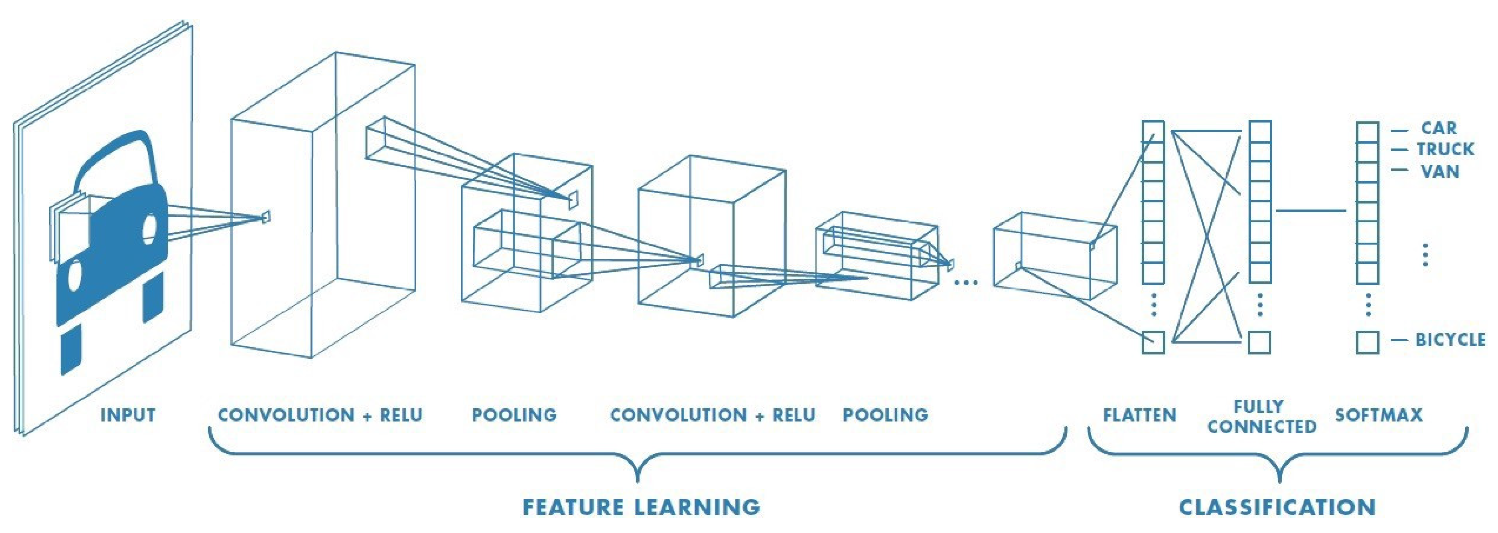
2. Convolutional Neural Networks
3. The SteGuz Approach
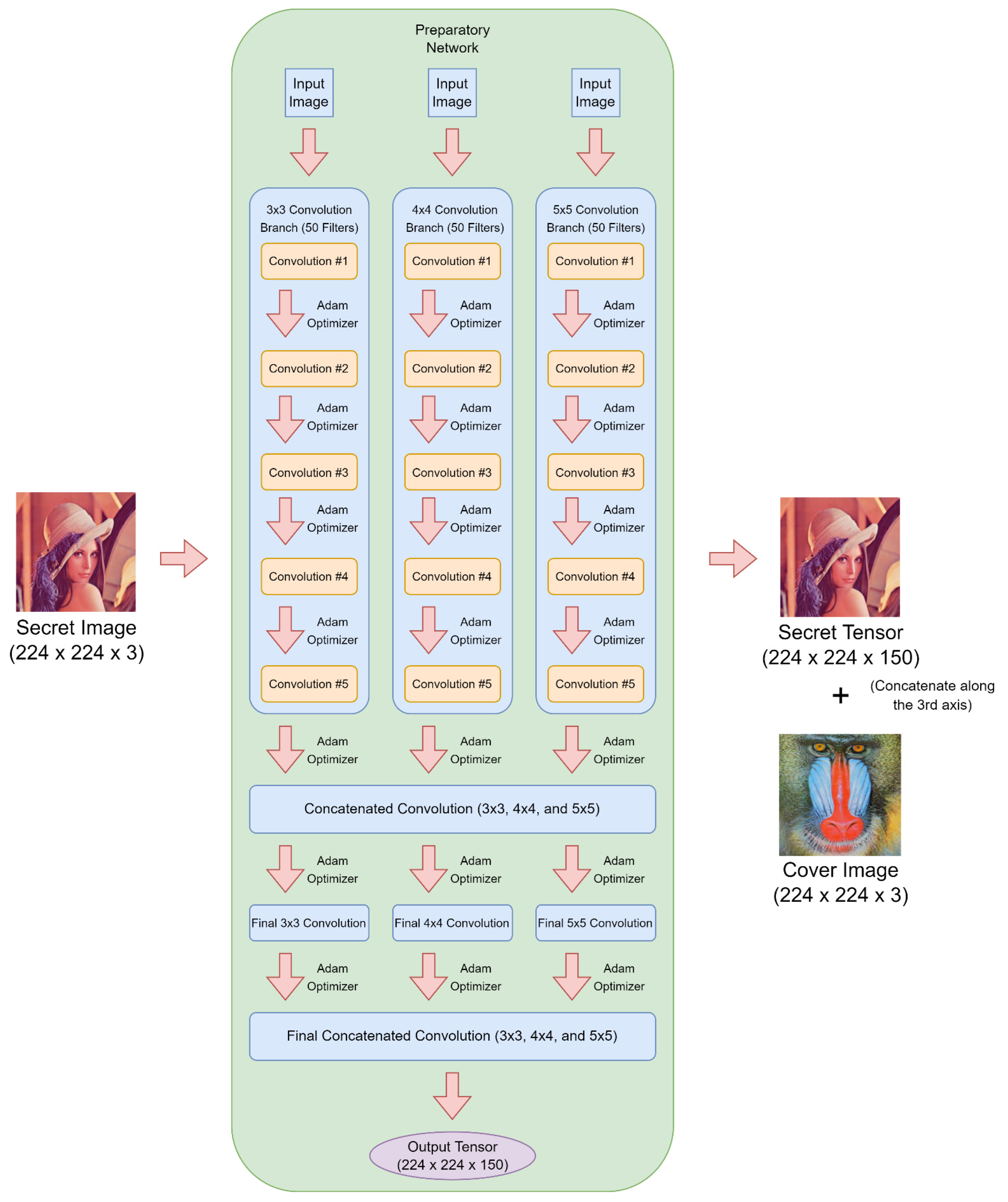
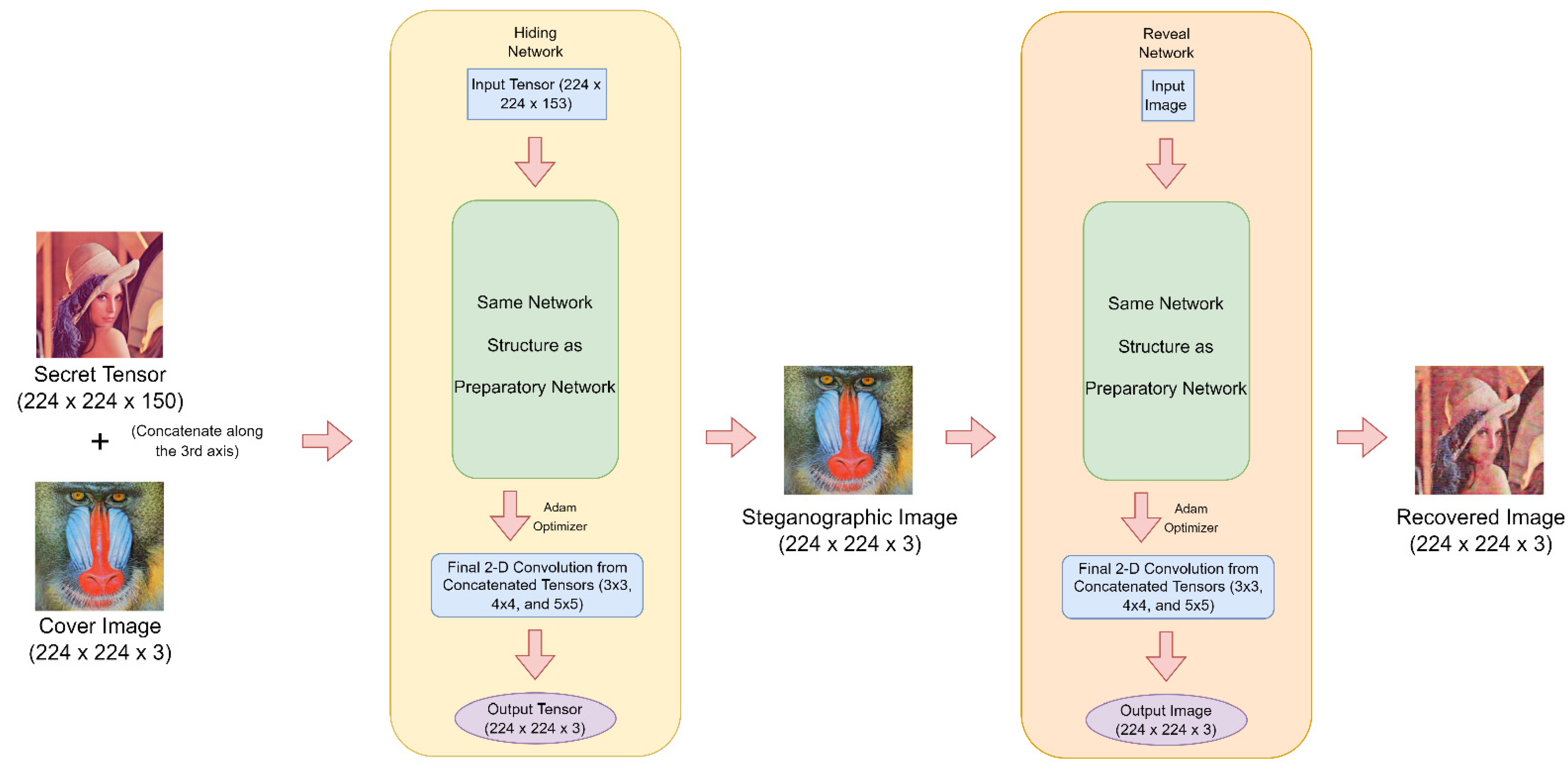
3.1. The Network Architecture
3.2. The Gain Function
3.3. The Model Hyperparameters
3.4. The Training Dataset
4. Results
4.1. The Experimental Setup
4.2. Objective Performance Measures
4.3. Experiemental Results
5. Discussion
6. Conclusions
Author Contributions
Funding
Institutional Review Board Statement
Informed Consent Statement
Data Availability Statement
Acknowledgments
Conflicts of Interest
References
- Jamil, T. Steganography: The art of hiding information in plain sight. IEEE Potentials 1999, 18, 10–12. [Google Scholar] [CrossRef]
- Cox, I.; Miller, M.; Bloom, J.; Fridrich, J.; Kalker, T. Digital Watermarking and Steganography; Elsevier Science & Technology: San Francisco, CA, USA, 2007. [Google Scholar]
- Artz, D. Digital steganography: Hiding data within data. IEEE Internet Comput. 2001, 5, 75–80. [Google Scholar] [CrossRef]
- What Is Bit Depth? Available online: https://etc.usf.edu/techease/win/images/what-is-bit-depth/ (accessed on 3 April 2022).
- Kasapbaşi, M.C.; Elmasry, W. New LSB-based colour image steganography method to enhance the efficiency in payload capacity, security and integrity check. Sādhanā 2018, 43, 68. [Google Scholar] [CrossRef] [Green Version]
- Ghazanfari, K.; Ghaemmaghami, S.; Khosravi, S.R. LSB++: An Improvement to LSB+ Steganography. In Proceedings of the IEEE Region 10 International Conference, Bali, Indonesia, 21–24 November 2011. [Google Scholar]
- Pradhan, A.; Sekhar, K.R.; Swain, G. Digital Image Steganography Using LSB Substitution, PVD, and EMD. Math. Probl. Eng. 2018, 2018, 1804953. [Google Scholar] [CrossRef]
- Chen, W.-Y. Color image steganography scheme using set partitioning in hierarchical trees coding, digital Fourier transform and adaptive phase modulation. Appl. Math. Comput. 2007, 185, 432–448. [Google Scholar] [CrossRef]
- Time Series, Signals, & the Fourier Transform, towards Data Science. Available online: https://towardsdatascience.com/time-series-signals-the-fourier-transform-f68e8a97c1c2 (accessed on 3 October 2021).
- Lin, C.-C.; Shiu, P.-F. High capacity data hiding scheme for DCT-based images. J. Inf. Hiding Multimed. Signal Process. 2010, 1, 220–240. [Google Scholar]
- Hamad, S.; Khalifa, A.; Elhadad, A. A Blind High-Capacity Wavelet-Based Steganography Technique for Hiding Images into other Images. Adv. Electr. Comput. Eng. 2014, 14, 35–42. [Google Scholar] [CrossRef]
- The Wavelet Transform. An Introduction and Example, Towards Data Science. Available online: https://towardsdatascience.com/the-wavelet-transform-e9cfa85d7b34 (accessed on 3 October 2021).
- Thanki, R.; Borra, S. A color image steganography in hybrid FRT–DWT domain. J. Inf. Secur. Appl. 2018, 40, 92–102. [Google Scholar] [CrossRef]
- Zhou, X.; Zhang, H.; Wang, C. A Robust Image Watermarking Technique Based on DWT, APDCBT, and SVD. Symmetry 2018, 10, 77. [Google Scholar] [CrossRef] [Green Version]
- Baluja, S. Hiding Images in Plain Sight: Deep Steganography. In Proceedings of the 31st Conference on Neural Information Processing Systems, Long Beach, CA, USA, 4–9 December 2017. [Google Scholar]
- Duan, X.; Guo, D.; Liu, N.; Li, B.; Gou, M.; Qin, C. A New High Capacity Image Steganography Method Combined With Image Elliptic Curve Cryptography and Deep Neural Network. IEEE Access 2020, 8, 25777–25788. [Google Scholar] [CrossRef]
- Volkhonskiy, D.; Nazarov, I.; Evgeny, B. Steganographic Generative Adversarial Networks. Int. Soc. Opt. Photonics 2020, 11433, 114333M. [Google Scholar] [CrossRef]
- Liu, M.-Y.; Tuzel, O. Coupled generative adversarial networks. In Proceedings of the 2016 Conference on Neural Information Processing Systems (NIPS 2016), Barcelona, Spain, 5–10 December 2016. [Google Scholar]
- Explained: Neural Networks. Available online: https://news.mit.edu/2017/explained-neural-networks-deep-learning-0414 (accessed on 19 September 2021).
- Everything You Need to Know about Neural Networks and Backpropagation—Machine Learning Easy and Fun. Available online: https://towardsdatascience.com/everything-you-need-to-know-about-neural-networks-and-backpropagation-machine-learning-made-easy-e5285bc2be3a (accessed on 19 September 2021).
- Rosenblatt, F. The perceptron: A probabilistic model for information storage and organization in the brain. Psychol. Rev. 1958, 65, 386–408. [Google Scholar] [CrossRef] [Green Version]
- How Do Convolutional Layers Work in Deep Learning Neural Networks. Available online: https://machinelearningmastery.com/convolutional-layers-for-deep-learning-neural-networks/ (accessed on 19 September 2021).
- Towards Data Science. Available online: https://towardsdatascience.com/a-comprehensive-guide-to-convolutional-neural-networks-the-eli5-way-3bd2b1164a53 (accessed on 26 February 2022).
- Everything You Need to Know about Gradient Descent Applied to Neural Networks. Available online: https://medium.com/yottabytes/everything-you-need-to-know-about-gradient-descent-applied-to-neural-networks-d70f85e0cc14 (accessed on 26 March 2022).
- IBM. What Is Gradient Descent? 27 October 2020. Available online: https://www.ibm.com/cloud/learn/gradient-descent (accessed on 27 March 2022).
- Wang, Z.; Simoncelli, E.P.; Bovik, A.C. Multiscale structural similarity for image quality assessment. In Proceedings of the Thrity-Seventh Asilomar Conference on Signals, Systems & Computers, Pacific Grove, CA, USA, 9–12 November 2003. [Google Scholar]
- Kingma, D.P.; Ba, J. Adam: A Method for Stochastic Optimization. In Proceedings of the International Conference for Learning Representations (ICLR 2015), San Diego, CA, USA, 7–9 May 2015. [Google Scholar]
- Hiding Images Using AI—Deep Steganography. Available online: https://medium.com/buzzrobot/hiding-images-using-ai-deep-steganography-b7726bd58b06 (accessed on 10 January 2021).
- van der Walt, S.; Schönberger, J.L.; Nunez-Iglesias, J.D.; Boulogne, F.; Warner, J.; Yager, N.; Gouillart, E.; Yu, T. scikit-image: Image processing in Python. PeerJ 2014, 2, e453. [Google Scholar] [CrossRef]
- Hunter, J.D. Matplotlib: A 2D graphics environment. Comput. Sci. Eng. 2007, 9, 90–95. [Google Scholar] [CrossRef]
- Chaladze, G.; Kalatozishvili, L. Linnaeus 5 Dataset for Machine Learning. 2017. Available online: http://chaladze.com/l5/ (accessed on 12 April 2022).
- Howard, J. Imagenette. Available online: https://github.com/fastai/imagenette (accessed on 12 April 2022).
- Zakaria, A.A.; Hussain, M.; Wahab, A.W.A.; Idris, M.Y.I.; Abdullah, N.A.; Jung, K.-H. High-Capacity Image Steganography with Minimum Modified Bits Based on Data Mapping and LSB Substitution. Appl. Sci. 2018, 8, 2199. [Google Scholar] [CrossRef] [Green Version]
- Duan, X.; Nao, L.; Mengxiao, G.; Yue, D.; Xie, Z.; Ma, Y.; Qin, C. High-Capacity Image Steganography Based on Improved FC-DenseNet. IEEE Access 2020, 8, 170174–170182. [Google Scholar] [CrossRef]
- TensorFlow 2.0 Is Now Available! Available online: https://blog.tensorflow.org/2019/09/tensorflow-20-is-now-available.html (accessed on 10 June 2022).
- Chen, F.; Xing, Q.; Liu, F. Technology of Hiding and Protecting the Secret Image Based on Two-Channel Deep Hiding Network. IEEE Access 2020, 8, 21966–21979. [Google Scholar] [CrossRef]
- Duan, X.; Liu, N.; Gou, M.; Wang, W.; Qin, C. SteganoCNN: Image Steganography with Generalization Ability Based on Convolutional Neural Network. Entropy 2020, 22, 1140. [Google Scholar] [CrossRef] [PubMed]

| Cover Images | Secret Images | ||
|---|---|---|---|
 Baboon | 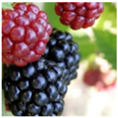 Berries | 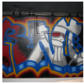 Graffiti | 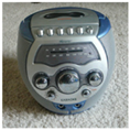 Karaoke |
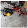 Chainsaws | 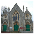 Church | 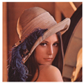 Lena | 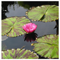 Lotus |
 Dog | 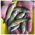 Fish | 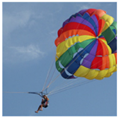 Parachute | 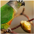 Parrot |
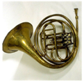 French Horn | 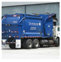 Garbage Truck | 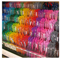 Pens | 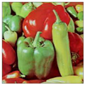 Peppers |
 Gas Pump | 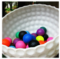 Golf Balls | 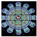 Stained Glass | 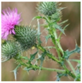 Thistle |
| Experiment | SteGuz | Deep Steganography [15] | ||
|---|---|---|---|---|
| Graffiti in Baboon | 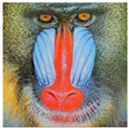 PSNR: 42.85748 | 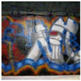 SSIM: 0.88449 | 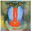 PSNR: 27.96642 | 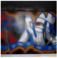 SSIM: 0.87001 |
| Karaoke in Berries | 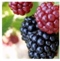 PSNR: 44.33152 | 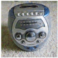 SSIM: 0.93213 | 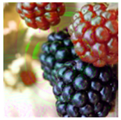 PSNR: 25.62975 | 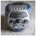 SSIM: 0.85424 |
| Lena in Chainsaws | 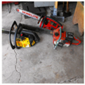 PSNR: 42.4834 |  SSIM: 0.91373 |  PSNR: 29.35 |  SSIM: 0.91303 |
| Lotus in Church |  PSNR: 44.17786 | 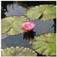 SSIM: 0.90252 |  PSNR: 29.59204 |  SSIM: 0.86413 |
| Parachute in Dog | 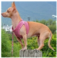 PSNR: 44.72544 | 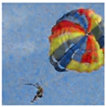 SSIM: 0.91306 | 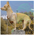 PSNR: 25.7312 | 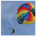 SSIM: 0.93006 |
| Parrot in Fish | 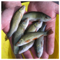 PSNR: 44.487 | 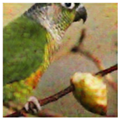 SSIM: 0.92739 | 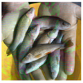 PSNR: 25.77007 | 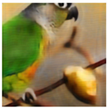 SSIM: 0.92166 |
| Pens in French Horn | 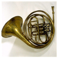 PSNR: 42.45224 | 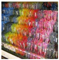 SSIM: 0.83423 | 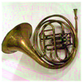 PSNR: 27.37058 |  SSIM: 0.77593 |
| Peppers in Garbage Truck | 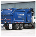 PSNR: 43.06884 | 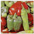 SSIM: 0.89151 | 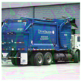 PSNR: 27.89983 | 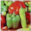 SSIM: 0.89549 |
| Stained Glass in Gas Pump |  PSNR: 41.65722 | 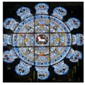 SSIM: 0.81930 | 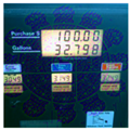 PSNR: 25.3442 | 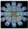 SSIM: 0.83418 |
| Thistle in Golf Balls | 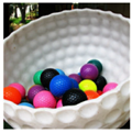 PSNR: 40.16172 | 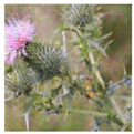 SSIM: 0.92120 | 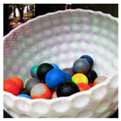 PSNR: 25.99714 | 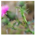 SSIM: 0.87267 |
| Method | Approach | Cover/Secret Images | Image Dataset | Cover vs. Stego-Image PSNR (db) | Secret vs. Retrieved Image Similarity | Hiding Capacity (bpp) |
|---|---|---|---|---|---|---|
| LSB | Spatial |  | N/A | 35.28 | 1 | 12 |
| TDHN [36] | CNN | 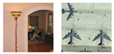 | NWPU-RESISC45 | 40.3 | 0.98 | 24 |
| FCDNet [34] | FC-DenseNet | 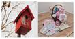 | ImageNet | 40.196 | 0.984 | 23.96 |
| SteganoCNN [37] | CNN |  | ImageNet | 21.614 | 0.855 | 48 |
| Deep Stego [15] | CNN |  | ImageNet | 28.69 | 0.73 | 24 |
| SteGuz | CNN | 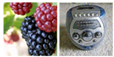 | Linnaeus 5/Imagenette | 44.33 | 0.93 | 24 |
Publisher’s Note: MDPI stays neutral with regard to jurisdictional claims in published maps and institutional affiliations. |
© 2022 by the authors. Licensee MDPI, Basel, Switzerland. This article is an open access article distributed under the terms and conditions of the Creative Commons Attribution (CC BY) license (https://creativecommons.org/licenses/by/4.0/).
Share and Cite
Khalifa, A.; Guzman, A. Imperceptible Image Steganography Using Symmetry-Adapted Deep Learning Techniques. Symmetry 2022, 14, 1325. https://doi.org/10.3390/sym14071325
Khalifa A, Guzman A. Imperceptible Image Steganography Using Symmetry-Adapted Deep Learning Techniques. Symmetry. 2022; 14(7):1325. https://doi.org/10.3390/sym14071325
Chicago/Turabian StyleKhalifa, Amal, and Anthony Guzman. 2022. "Imperceptible Image Steganography Using Symmetry-Adapted Deep Learning Techniques" Symmetry 14, no. 7: 1325. https://doi.org/10.3390/sym14071325
APA StyleKhalifa, A., & Guzman, A. (2022). Imperceptible Image Steganography Using Symmetry-Adapted Deep Learning Techniques. Symmetry, 14(7), 1325. https://doi.org/10.3390/sym14071325