Stress Point Monitoring Algorithm for Structure of Steel Cylinder Concrete Pipes in Large Buildings

Abstract

The internal structure of steel cylinder concrete pipe in large buildings is complex. Traditionally, the safety monitoring method is unable to accurately monitor the situation of every stress point in the structure. Therefore, the wireless sensor network with practical value in the field of building safety monitoring was introduced. A monitoring algorithm for stress points in pipeline structure was put forward. The distribution law of circumferential prestress produced by prestress steel wire on the pipe core concrete was analyzed. According to the influencing factors, the mechanical performance of tube concrete pipe structure was discussed, and the method of calculating prestress of pipe structure was constructed. Combined with sensor network nodes, a series of basic hypothesis information was set. Moreover, the force between node and stress point was analyzed by virtual potential field. Based on the force analysis for the centroid of the sensing area, the monitoring of the stress point in pipeline structures was completed. After that, a rectangular area to be monitored was selected and the force points were established randomly. According to the relationship between network coverage rate and monitoring efficiency, we found that the proposed algorithm had good network immunity. According to the different number of nodes, sensing radii and perception angles, the influence of index on the monitoring accuracy was discussed. Experimental results show that the accuracy of the proposed algorithm is sensitive to the change of node parameter. When the number of nodes, sensing radius and sensing angle change, the maximum fluctuation range of monitoring accuracy is 0.08–0.99. From the application effect of the algorithm, we can see that the detection effect of the algorithm has obvious advantage.

1. Introduction

Prestressed concrete cylinder pipe (PCCP) is widely used in hydraulic engineering, industrial water supply and other fields [1]. Since its birth in the 18th century, PCCP pipe has been widely used in municipal engineering, electric power engineering and water conservancy projects. PCCP pipeline was introduced into China in the mid-1980s. After more than twenty years of development, specifications and systems have been initially formed. In view of the excellent performance, PCCP pipeline is favored in domestic engineering application. Firstly, the concrete is poured on the inner or outer sides of the steel cylinder to form a concrete pipe core, and then the prestressed steel wire is wound on the concrete pipe core. Finally, a layer of mortar protective layer is sprayed. The spigot joints, steel cylinder and rubber ring at both ends of the pipe form a sealing member to ensure the tightness of pipe [2,3]. The safety and stability of pipeline in the application process is particularly important. According to the actual situation of large construction projects, it is necessary to reasonably analyze the stress distribution of pipeline and monitor the stress points in pipeline structure, so as to provide reference for the actual engineering. Therefore, relevant researchers have carried out the following explorations on PCCP.

Reference [4] studies the deformation law of PCCP under extreme external load. BOTDA (Brillouin optical time domain analyzer) and FBG (Fiber Bragg Grating) Optical fiber sensing technologies are adopted for the first time at home and abroad, and the optical fiber is implanted into the surface of steel cylinder in the manufacturing process of PCCP. The external load test of embedded PCCP prototype tube with inner diameter of 2.6 m is carried out by the three-point test method, and the strain response of each layer structure of PCCP is continuously tested during the loading process. This study only analyzes the external load of PCCP pipe and ignores the analysis of the load in other directions. Therefore, reference [5] establishes the soil load model of concrete pipeline after failure by analyzing the variation law of soil load in three stages of pipeline construction, use and failure. In the established model, the soil load on the top of the pipe is calculated according to the soil column load, the soil load on the bottom of the pipe is calculated according to the uniformly distributed load, the pipe side load is equal to the sum of the static side soil load and the triangular distributed load, and the circumferential internal force coefficient of the pipe wall is calculated according to the newly established model, which provides a reference for the trenchless structural repair design of concrete pipeline. Although the research has obtained good stress analysis results, it cannot realize the visualization of the PCCP pressure bearing process. Therefore, based on the action mechanism of annular prestress, reference [6] compared the negative pressure borne by PCCP to the circumferential force, calculated and analyzed the capacity of PCCP to bear negative pressure, established the model under the actual embedded conditions through the finite element software ABAQUS, and selected the appropriate material constitution for numerical simulation. The calculation results are consistent with the theoretical calculation results. Reference [7] suggested that prestressed wire breakage may lead to pipeline rupture and serious disaster. The application of adhering carbon fiber reinforced plastics (CFRP) lining to the interior of concrete is an effective method for internal repair and reinforcement of PCCP. The structural performance of PCCP lined with CFRP is studied through the comprehensive experimental test and corresponding finite element model evaluation, and the failure risk analysis method is introduced to determine the number of CFRP layers required for poor PCCP.

The stability of the building is not only related to the lifetime of the building, but also related to the safety of the surrounding people. Once the building collapses, it will cause great loss to economic property. Due to the complexity of internal structure of cylinder concrete pipes, the traditional safety monitoring method has many defects. The application of wireless sensor network in the field of building safety monitoring provides more reliable and efficient disaster prevention measures [8].

Due to the complex working environment of PCCP pipe, the structure itself will produce cracks and broken wires, which will affect the bearing performance of the pipe, and even lead to engineering accidents such as pipe explosion in serious cases. Therefore, it is necessary to analyze the pressure bearing capacity of PCCP pipe. At present, the mechanical performance analysis methods of steel tube concrete pipeline regard the pipeline structure as a whole. Although good mechanical analysis results have been obtained, it is unable to accurately monitor the situation of each force point in the structure. Therefore, this paper introduces the wireless sensor network with practical value in the field of building safety monitoring, and designs a force point monitoring algorithm of large-scale building steel tube concrete pipeline structure. Some sensor nodes are installed in the pipeline, which can automatically collect and report the index data of stress point in the pipeline structure. A series of basic hypothesis information is set innovatively. The virtual potential field is used to analyze the force between node and stress point, and then the force on the centroid of the sensing area is analyzed. The monitoring for the stress point in pipeline structures is completed. This study can effectively improve the stability of buildings and reduce personnel damage and property loss caused by building collapse.

2. Structural Performance of Structure of Concrete Cylinder Pipe in Large Buildings

In order to obtain better monitoring effect, it is necessary to analyze the mechanical performance of concrete cylinder pipe structures. PCCP has a strong pressure bearing capacity. In addition to its own structural characteristics, the initial compressive stress generated by prestressed high-strength steel wire on the pipe core concrete is also very important. When the pipe core concrete is subjected to internal water pressure, it will not be tensioned until the prestress is offset. Thus, the pressure bearing capacity of PCCP can be improved [9].

According to the manufacturing process of PCCP, the prestressed steel wire is wrapped on the pipe core concrete, and then it is sprayed with mortar protective layer, so the prestressed steel wire will not produce prestress on the mortar protective layer. When analyzing the stress point of PCCP pipe, the mortar protective unit should be ignored, so that only the inner and outer core concrete, steel cylinder and prestressed steel wire are included in the calculation model [10,11].

2.1. Influence of Buried Depth on Stress of Cylinder Concrete Pipe

The buried depth is one of the important factors influencing the mechanical performance of PCCP. Five buried depths (3 m, 4 m, 5 m, 6 m, 7 m) were designed [12]. It is assumed that the internal water pressure on the pipe is 0.6 MPa, the wall thickness is 300 mm and the concrete strength grade is C40. According to the method of calculating soil load, the soil load value was calculated, and then applied to the pipeline. The extreme stress of the layer of PCCP in different buried depths is shown in

Table 1. Extreme stress of layers of prestressed concrete cylinder pipe (PCCP) in different buried depths (MPa).

Location.	Inner Tube Core Concrete		Outer Tube Core Concrete		Steel Cylinder		Mortar Protective Course
Buried Depth	Maximum Stress	Minimum Stress	Maximum Stress	Minimum Stress	Maximum Stress	Minimum Stress	Maximum Stress	Minimum Stress
3 m	−1.56	−11.1	−1.82	−8.05	−24.5	−48.2	0.230	−7.53
5 m	0.583	−14.3	−0.234	−10.0	−20.6	−57.4	0.813	−9.58
6 m	1.66	−16.0	0.564	−11.0	−18.6	−61.9	1.68	−10.6
7 m	*	−17.6	1.36	−12.0	−16.7	−66.5	*	−11.6

Note: “−” indicates that it is in compression; “*” indicates exceeding the standard strength of the material.

. The maximum compressive stress of pipe core concrete and steel cylinder appeared at the inner side of the inner concrete pipe when the buried depth was 7 m. The maximum compressive stress of pipe core concrete is 17.6 MPa [13,14,15]. The maximum compressive stress of steel cylinder is 66.5 MPa. The values are less than the standard value of compressive strength.

2.2. Influence of Internal Water Pressure on the Stress of Cylinder Concrete Pipe

The internal water pressure is also an important factor influencing the mechanical performance of PCCP. Four levels of internal water pressure (0.6 MPa, 0.7 MPa, 0.8 MPa and 0.84 MPa) were selected for analysis. It is assumed that the buried depth of pipeline is 5 m, the thickness of pipe wall is 300 mm, and the concrete strength grade is C40. The extreme stresses of the layers of PCCP in different internal water pressures are shown in

Table 2. Extremum of layers of PCCP in different internal water pressure (MPa).

Location	Inner Tube Core Concrete		Outer Tube Core Concrete		Steel Cylinder		Mortar Protective Course
Inner Pressure	Maximum Stress	Minimum Stress	Maximum Stress	Minimum Stress	Maximum Stress	Minimum Stress	Maximum Stress	Minimum Stress
0.6 MPa	0.583	−14.3	−0.234	−10.0	−20.6	−57.4	0.813	−9.58
0.7 MPa	1.35	−13.6	0.416	−9.42	−12.8	−52.7	1.41	−9.01
0.8 MPa	2.01	−12.9	1.07	−8.80	−11.1	−48.1	2.11	−8.45
0.84 MPa	*	−12.7	1.33	−8.56	−9.19	−46.2	*	−8.22

Note: “−” indicates that it is in compression; “*” indicates exceeding the standard strength of the material.

.

2.3. Influence of Wall Thickness on Stress of Cylinder Concrete Pipe

The thickness of pipe wall is also an important factor influencing the mechanical performance of PCCP. Four wall thicknesses (260 mm, 280 mm, 300 mm and 320 mm) are selected [16]. It is assumed that the buried depth of pipeline is 5 m, the internal water pressure is 0.6 MPa, and the concrete strength grade is C40. The extreme stress in each layer of PCCP under different wall thickness is shown in

Table 3. Extreme stress of PCCP layers in different pipe wall thickness (MPa).

Location	Inner Tube Core Concrete		Outer Tube Core Concrete		Steel Cylinder		Mortar Protective Course
Wall Thickness	Maximum Stress	Minimum Stress	Maximum Stress	Minimum Stress	Maximum Stress	Minimum Stress	Maximum Stress	Minimum Stress
260 mm	0.981	−16.8	0.0844	−11.7	−19.6	−71.2	1.41	−11.3
280 mm	0.749	−15.5	0.0978	−10.8	−19.8	−64.3	1.07	−10.4
300 mm	0.583	−14.3	−0.234	−10.0	−20.6	−57.4	0.813	−9.58
320 mm	0.430	−13.4	−0.350	−9.35	−19.5	−53.6	0.607	−8.81

.

2.4. Influence of Concrete Strength on Stress of Concrete Cylinder Pipe

According to CECS140:2002, the concrete strength grades (C40, C50 and C60) are designed [17]. The buried depth of pipeline is 5 m, the internal water pressure is 0.6 MPa, and the thickness of pipe wall is 300 mm. The extreme stress of each layer of PCCP in different concrete strength grades is shown in

Table 4. Extreme stress of PCCP layers in different concrete strength grades (MPa).

Location	Inner Tube Core Concrete		Outer Tube Core Concrete		Steel Cylinder		Mortar Protective Course		Prestressed Wire
Inner Pressure	Maximum Stress	Minimum Stress	Maximum Stress	Minimum Stress	Maximum Stress	Minimum Stress	Maximum Stress	Minimum Stress
C40	0.583	−14.3	−0.234	−10.0	−20.6	−57.4	0.813	−9.58	1110
C50	0.824	−15.6	0.017	−11.0	−18.7	−61.1	1.13	−9.96	1150
C60	0.880	−15.8	0.101	−11.1	−18.0	−58.9	1.16	−9.67	1150

Note: “−“ means pressure.

.

2.5. Calculation and Analysis of Prestress Design

The cross-section area ${\mathrm{A}}_{\mathrm{y}}$ of circumferential prestressed steel wire required per unit length of PCCP is:

$${\mathrm{A}}_{\mathrm{y}}\ge \frac{\left({\mathrm{r}}_{\mathrm{p}}^2+{\mathrm{r}}_1^2\right){\mathrm{P}}_{\mathrm{hd}}-\left({\mathrm{r}}_{\mathrm{p}}^2-{\mathrm{r}}_1^2\right)\left({\mathsf{\alpha }}_{\mathrm{ct}}{\mathrm{f}}_{\mathrm{tk}}+\frac{{\mathrm{M}}_{\mathrm{pms}}}{{\mathsf{\gamma }\mathsf{\omega }\mathrm{W}}_{\mathrm{p}}}\right)}{2{\mathrm{r}}_{\mathrm{p}}{\mathsf{\sigma }}_{\mathrm{pe}}}$$

(1)

In the formula, ${\mathrm{A}}_{\mathrm{y}}$ is the sectional area of prestressed steel wire per unit length of pipe (${\mathrm{mm}}^2/\mathrm{m}$); ${\mathsf{\sigma }}_{\mathrm{pe}}$ is the effective prestress of prestressed steel wire, ${\mathsf{\sigma }}_{\mathrm{pe}}={\mathsf{\sigma }}_{\mathrm{con}}-{\mathsf{\sigma }}_{\mathrm{l}}\mathsf{\sigma }$; ${\mathsf{\sigma }}_{\mathrm{con}}$ is the tension control stress of prestressed steel wire; ${\mathsf{\sigma }}_{\mathrm{l}}$ is the total prestress loss of steel wire; and ${\mathrm{P}}_{\mathrm{hd}}$ is the designed internal water pressure.

The cross-section area ${\mathrm{A}}_{\mathrm{y}}$ of circumferential prestress steel wire required per unit length of PCCP on pipe side is:

$${\mathrm{A}}_{\mathrm{y}}\ge \frac{\left[2{\mathrm{r}}_1^2{\mathrm{P}}_{\mathrm{hd}}-\left({\mathrm{r}}_2^2-{\mathrm{r}}_1^2\right)\left({\mathsf{\alpha }}_{\mathrm{ct}}{\mathrm{f}}_{\mathrm{tk}}+\frac{{\mathrm{M}}_{\mathrm{pms}}^1}{{\mathsf{\gamma }\mathsf{\omega }\mathrm{W}}_{\mathrm{cm}}}\right)\right]\ast {\mathrm{r}}_{\mathrm{p}}}{\left[\left({\mathrm{r}}_{\mathrm{p}}^2+{\mathrm{r}}_{\mathrm{q}}^2\right)-\frac{\mathsf{\mu }}{1-\mathsf{\mu }}\left({\mathrm{r}}_{\mathrm{p}}^2-{\mathrm{r}}_1^2\right)\right]{\mathsf{\sigma }}_{\mathrm{pe}}}$$

(2)

From above formulas, we can see that the area of prestressed steel wire is mainly related to the thickness of pipe wall, buried depth and internal water pressure. In order to meet the requirement that no cracking of pipeline occurred, it is suggested that the area of prestressed steel wire should be multiplied by the increasing factor λ.

Calculation section of pipe top and pipe bottom:

$${\mathrm{A}}_{\mathrm{y}}\ge \mathsf{\lambda }\frac{\left({\mathrm{r}}_{\mathrm{p}}^2+{\mathrm{r}}_1^2\right){\mathrm{P}}_{\mathrm{hd}}-\left({\mathrm{r}}_{\mathrm{p}}^2-{\mathrm{r}}_1^2\right)\left({\mathsf{\alpha }}_{\mathrm{ct}}{\mathrm{f}}_{\mathrm{tk}}+\frac{{\mathrm{M}}_{\mathrm{pms}}}{{\mathsf{\gamma }\mathsf{\omega }\mathrm{W}}_{\mathrm{p}}}\right)}{2{\mathrm{r}}_{\mathrm{p}}{\mathsf{\sigma }}_{\mathrm{pe}}}$$

(3)

The section on tube side:

$${\mathrm{A}}_{\mathrm{y}}\ge \mathsf{\lambda }\frac{\left[2{\mathrm{r}}_1^2{\mathrm{P}}_{\mathrm{hd}}-\left({\mathrm{r}}_2^2-{\mathrm{r}}_1^2\right)\left({\mathsf{\alpha }}_{\mathrm{ct}}{\mathrm{f}}_{\mathrm{tk}}+\frac{{\mathrm{M}}_{\mathrm{pms}}^1}{{\mathsf{\gamma }\mathsf{\omega }\mathrm{W}}_{\mathrm{cm}}}\right)\right]\ast {\mathrm{r}}_{\mathrm{P}}}{\left[\left({\mathrm{r}}_{\mathrm{P}}^2+{\mathrm{r}}_1^2\right)-\frac{\mathsf{\mu }}{1-\mathsf{\mu }}\left({\mathrm{r}}_{\mathrm{P}}^2-{\mathrm{r}}_1^2\right)\right]{\mathsf{\sigma }}_{\mathrm{pe}}}$$

(4)

3. An Algorithm of Monitoring Stress Point in Structure of Cylinder Concrete Pipe

Based on the above analysis of the mechanical performance of cylinder concrete pipe, the sensor network node is introduced to construct the monitoring algorithm [18].

3.1. Hypothesis and Perception Model

In the concrete-filled steel tubular pipe structure of large buildings, the sensing direction of nodes is limited. Therefore, it is set that the monitoring area is a sector symmetrical area with the node as the center of the circle and the sensing radius as the sensing distance. The sector symmetrical area can be switched to different directions around the center of the circle, and each direction can only perceive a limited range.

In order to facilitate the analysis, the research and design of algorithm should be based on the basic assumptions:

(1)

All nodes are isomorphic and symmetrical, that is, they have the same perception radius, angle and communication radius;

(2)

After the initial monitoring, the node can move and the sensing direction can be adjusted;

(3)

The node has known its own location information through a location algorithm;

(4)

The force point of node is its own position and the centroid of the fan-shaped sensing area. The force on the node changes its position, and the force on the center of mass changes its sensing direction.

The four tuples (${\mathrm{S}}_{\mathrm{i}},{\mathrm{r}}_{\mathrm{i}},{\mathrm{V}}_{\mathrm{i}},{\mathsf{\theta }}_{\mathrm{i}}$) denotes the perception model of node ${\mathrm{s}}_{\mathrm{i}}$, which is shown in Figure 1, where ${\mathrm{s}}_{\mathrm{i}}=\left({\mathrm{x}}_{\mathrm{i}},{\mathrm{y}}_{\mathrm{i}}\right)$ is the position coordinate of node ${\mathrm{s}}_{\mathrm{i}}$; ${\mathrm{r}}_{\mathrm{i}}$ is the effective sensing radius; ${\mathrm{V}}_{\mathrm{i}}$ is the main perceptual direction; and $2{\mathsf{\theta }}_{\mathrm{i}}$ is the maximum perception angle. The node sensing model is shown in Figure 1.

In the operating stage of the network, with the change of node position and direction, the force point ${\mathrm{t}}_{\mathrm{m}}$ and node ${\mathrm{s}}_{\mathrm{i}}$ should satisfy the following constraints: Euclidean distance from node ${\mathrm{s}}_{\mathrm{i}}$ to force point ${\mathrm{t}}_{\mathrm{m}}$ is $\Vert {\mathrm{s}}_{\mathrm{i}}{\mathrm{t}}_{\mathrm{m}}\Vert \le {\mathrm{r}}_{\mathrm{i}}$. The value range of intersection angle between ${\mathrm{s}}_{\mathrm{i}}{\mathrm{t}}_{\mathrm{m}}$ and ${\mathrm{V}}_{\mathrm{i}}$ is $\left[-\mathsf{\theta },\mathsf{\theta }\right]$, and then the node ${\mathrm{s}}_{\mathrm{i}}$ monitors the force point ${\mathrm{t}}_{\mathrm{m}}$. In the monitoring process, if a pressure point ${\mathrm{t}}_{\mathrm{m}}$ is monitored by k nodes at the same time, the stress point is monitored for k times.

3.2. Force Analysis of Pressure Points

In order to obtain accurate and comprehensive information, the multiple and priority monitoring method is adopted for the stressed target with high monitoring quality. However, the whole area to be monitored does not want to be monitored in multiple ways. Therefore, the virtual potential field is introduced, so that the sensor nodes can move and adjust their own direction under the force, and thus complete the monitoring for the force bearing point. Meanwhile, we can consider regional monitoring.

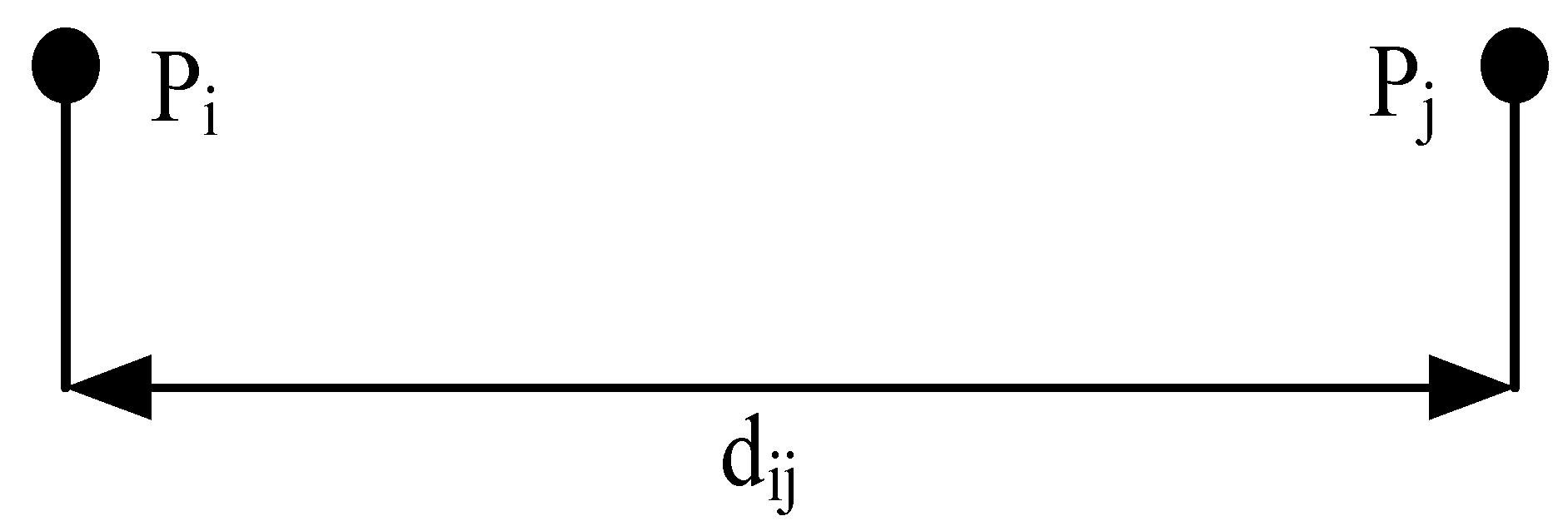
3.2.1. Principle of Virtual Potential Field

The principle of virtual potential field shows that each node or force point in the network is regarded as a virtual charged particle, and there is interaction between adjacent particles. In Figure 2, ${\mathrm{d}}_{\mathrm{ij}}$ is the distance between particle ${\mathrm{P}}_{\mathrm{i}}$ and particle ${\mathrm{P}}_{\mathrm{j}}$ [19,20].

When the distance between two particles is very close, the repulsive force between the two particles is shown. When the particle is far away from each other, the attraction between the two particles is shown [21]. Under the resultant force, particles move freely and the distance between particles can be adjusted to the best state. The nodes and stress points are regarded as the charged particles in the potential field. By establishing the force relation between nodes, and the force relation between nodes and stress points, the position and sensing direction of sensor node are determined by the force balance between the center of circle and the center of mass [22,23,24].

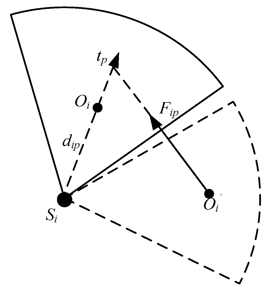
3.2.2. Mechanical Analysis of Node

During the self-organization movement of node, in order to facilitate the calculation, the dominant force between non-neighbor nodes is defined as gravity, and the effect of repulsive force is ignored [25,26,27]. If the repulsive force between neighbor nodes is the dominant force, the effect of gravity is also ignored. Let us assume $\mathrm{S}=\left\{{\mathrm{s}}_1,{\mathrm{s}}_2,\dots ,{\mathrm{s}}_{\mathrm{n}}\right\}$ to be the set of nodes in the area to be monitored. The Euclidean distance between node ${\mathrm{s}}_{\mathrm{i}}$ and node ${\mathrm{s}}_{\mathrm{j}}$ can be expressed as ${\mathrm{d}}_{\mathrm{ij}}=\Vert {\mathrm{s}}_{\mathrm{i}}{\mathrm{s}}_{\mathrm{j}}\Vert \left(1\le \mathrm{i}\le \mathrm{n},1\le \mathrm{j}\le \mathrm{n}\right)$. ${\mathrm{d}}_{\mathrm{th}}$ denotes the best distance between two nodes, which is used to adjust the property of the force between two nodes. The azimuth between node ${\mathrm{s}}_{\mathrm{i}}$ and node ${\mathrm{s}}_{\mathrm{j}}$ is expressed by ${\mathsf{\alpha }}_{\mathrm{ij}}$. The communication radius is $\mathrm{R}$ [28,29]. Thus, the force between two nodes can be expressed as follows:

$${\mathrm{F}}_{\mathrm{ij}}=\{\begin{array}{c}\left({\mathrm{w}}_{\mathrm{r}}\left(\frac{1}{{\mathrm{d}}_{\mathrm{ij}}}-\frac{1}{{\mathrm{d}}_{\mathrm{th}}}\right),{\mathsf{\alpha }}_{\mathrm{ij}}+\mathsf{\pi }\right),{\mathrm{d}}_{\mathrm{ij}}<{\mathrm{d}}_{\mathrm{th}}\\ 0,{\mathrm{d}}_{\mathrm{ij}}={\mathrm{d}}_{\mathrm{th}}\\ \left({\mathrm{w}}_{\mathsf{\alpha }}\left({\mathrm{d}}_{\mathrm{ij}}-{\mathrm{d}}_{\mathrm{th}}\right),{\mathsf{\alpha }}_{\mathrm{ij}}\right),{\mathrm{d}}_{\mathrm{th}}<{\mathrm{d}}_{\mathrm{ij}}<\mathrm{R}\\ 0,{\mathrm{d}}_{\mathrm{ij}}\ge \mathrm{R}\end{array}$$

(5)

In the formula, ${\mathrm{w}}_{\mathrm{r}}$ and ${\mathrm{w}}_{\mathsf{\alpha }}$ are the repulsive force and gravitational coefficient between nodes, which are used to adjust the density of nodes. Generally, they are determined by experience.

In addition to the interaction force between nodes, the force point in the region to be monitored is also analogous to the charged particles in the potential field, which has the same effect on the nodes. Let us assume that $\mathrm{T}=\left({\mathrm{t}}_1,{\mathrm{t}}_2,\dots ,{\mathrm{t}}_{\mathrm{m}}\right)$ is the set of pressure points, then the force of ${\mathrm{t}}_{\mathrm{p}}\left(1\le \mathrm{p}\le \mathrm{m}\right)$ on node ${\mathrm{s}}_{\mathrm{i}}$ can be expressed as:

$${\mathrm{F}}_{\mathrm{ip}}=\{\begin{array}{c}0,{\mathrm{d}}_{\mathrm{ip}}<\mathrm{r}\\ \left(\mathrm{w}\left({\mathrm{d}}_{\mathrm{ip}}-\mathrm{r}\right),{\mathsf{\alpha }}_{\mathrm{ip}}\right),\mathrm{r}\le {\mathrm{d}}_{\mathrm{ip}}\le 2\mathrm{r}\\ 0,{\mathrm{d}}_{\mathrm{ip}}>2\mathrm{r}\end{array}$$

(6)

In the formula, $\mathrm{r}$ is the sensing radius of node; ${\mathrm{d}}_{\mathrm{ip}}$ is the distance between target ${\mathrm{t}}_{\mathrm{p}}$ and node ${\mathrm{s}}_{\mathrm{i}}$; $\mathrm{w}$ is the coefficient of attractive force of pressure point to node; and ${\mathsf{\alpha }}_{\mathrm{ip}}$ is the azimuth between node ${\mathrm{s}}_{\mathrm{i}}$ and pressure point ${\mathrm{t}}_{\mathrm{p}}$. Due to the particularity of force point, the repulsive effect on the node is ignored. When ${\mathrm{d}}_{\mathrm{ip}}>2\mathrm{r}$, due to the energy consumption of node motion, the force acting on the node is zero. For node ${\mathrm{s}}_{\mathrm{i}}$, the resultant force of other nodes and pressure points on node ${\mathrm{s}}_{\mathrm{i}}$ is expressed as follows:

$${\mathrm{F}}_{\mathrm{i}}={{\displaystyle \sum }}_{\mathrm{j}=1,\mathrm{j}\ne \mathrm{i}}^{\mathrm{k}}{\mathrm{F}}_{\mathrm{ij}}+{{\displaystyle \sum }}_{\mathrm{p}=1}^{\mathrm{m}}{\mathrm{F}}_{\mathrm{ip}}$$

(7)

where $\mathrm{k}$ is the number of neighbor nodes of node ${\mathrm{s}}_{\mathrm{i}}$, and m is the number of forces bearing points. The direction of ${\mathrm{F}}_{\mathrm{i}}$ is determined by the vector and direction of virtual force on node ${\mathrm{s}}_{\mathrm{i}}$.

According to the force on node ${\mathrm{s}}_{\mathrm{i}}$, the kinematic equation is obtained.

$${\mathrm{a}}_{\mathrm{i}}=\frac{{\mathrm{F}}_{\mathrm{i}}-{\mathsf{\mu }\mathrm{v}}_{\mathrm{i}}}{\mathrm{m}}$$

(8)

In the formula, ${\mathrm{a}}_{\mathrm{i}}$ is the acceleration of node ${\mathrm{s}}_{\mathrm{i}}$; ${\mathrm{v}}_{\mathrm{i}}$ is the velocity; μ is the resistance coefficient; and m is the node mass. After the initial placement, the nodes begin to move in a self-organization way under the action of force, but its speed cannot increase infinitely. When the node speed increases to the maximum threshold, its speed does not increase any more, but moves at a constant speed. The displacement of node ${\mathrm{s}}_{\mathrm{i}}$ in x and y directions is expressed as follows:

$$\Delta {\mathrm{sx}}_{\mathrm{i}}=\{\begin{array}{c}{\mathrm{v}}_{\mathrm{ix}}\times \Delta \mathrm{t}+\frac{1}{2}\times {\mathrm{a}}_{\mathrm{ix}}\times \Delta {\mathrm{t}}^2,{\mathrm{v}}_{\mathrm{ix}}<{\mathrm{v}}_{\mathrm{jxmax}}\\ {\mathrm{v}}_{\mathrm{ix}}\times \Delta \mathrm{t},{\mathrm{v}}_{\mathrm{ix}}={\mathrm{v}}_{\mathrm{ixmax}}\end{array}$$

(9)

$$\Delta {\mathrm{sy}}_{\mathrm{i}}=\{\begin{array}{c}{\mathrm{v}}_{\mathrm{iy}}\times \Delta \mathrm{t}+\frac{1}{2}\times {\mathrm{a}}_{\mathrm{iy}}\times \Delta {\mathrm{t}}^2,{\mathrm{v}}_{\mathrm{iy}}<{\mathrm{v}}_{\mathrm{iymax}}\\ {\mathrm{v}}_{\mathrm{iy}}\times \Delta \mathrm{t},{\mathrm{v}}_{\mathrm{iy}}={\mathrm{v}}_{\mathrm{iymax}}\end{array}$$

(10)

where ${\mathrm{v}}_{\mathrm{ix}}$ and ${\mathrm{a}}_{\mathrm{ix}}$ are velocity and acceleration of node ${\mathrm{s}}_{\mathrm{i}}$ in x and y directions; ${\mathrm{v}}_{\mathrm{iy}}$ and ${\mathrm{a}}_{\mathrm{iy}}$ are velocity and acceleration of node ${\mathrm{s}}_{\mathrm{i}}$ in x and y directions; and $\Delta \mathrm{t}$ is the time step.

Therefore, the updated position of node ${\mathrm{s}}_{\mathrm{i}}$ is expressed as follows:

$${\mathrm{x}}_{\mathrm{i}\_\mathrm{new}}=\{\begin{array}{c}{\mathrm{x}}_{\mathrm{i}\_\mathrm{old}},\left|{\mathrm{F}}_{\mathrm{ix}}\right|\le {\mathrm{F}}_{\mathrm{th}}\\ {\mathrm{x}}_{\mathrm{i}\_\mathrm{old}}+\Delta {\mathrm{sx}}_{\mathrm{i}},\left|{\mathrm{F}}_{\mathrm{ix}}\right|>{\mathrm{F}}_{\mathrm{th}}\end{array}$$

(11)

$${\mathrm{y}}_{\mathrm{i}\_\mathrm{new}}=\{\begin{array}{c}{\mathrm{y}}_{\mathrm{i}\_\mathrm{old}},\left|{\mathrm{F}}_{\mathrm{iy}}\right|\le {\mathrm{F}}_{\mathrm{th}}\\ {\mathrm{y}}_{\mathrm{i}\_\mathrm{old}}+\Delta {\mathrm{sy}}_{\mathrm{i}},\left|{\mathrm{F}}_{\mathrm{iy}}\right|>{\mathrm{F}}_{\mathrm{th}}\end{array}$$

(12)

where ${\mathrm{F}}_{\mathrm{ix}}$ and ${\mathrm{F}}_{\mathrm{iy}}$ are the components of resultant force of node ${\mathrm{s}}_{\mathrm{i}}$ in x and y directions, and ${\mathrm{F}}_{\mathrm{th}}$ is the virtual force threshold.

3.2.3. Force Analysis of Centroid of Sensing Area

For the directional sensing model, the continuous adjustment of sensing direction can be regarded as a circular motion of the centroid of the sector sensing region around the node. The centroid is located on the symmetry axis of sector region, and the distance from the center of the circle is 2rsinθ/sin3θ ($\mathrm{r}$ is the sensing radius, and $\mathsf{\theta }$ is half of the perception angle). The centroid is analogous to a charged particle in a virtual potential field, and the force adjusts the sensing direction of node.

The redundant monitoring data may appear only when the two nodes are neighbors to each other; in this case, the repulsive force model is used for the force acting on the centroid between nodes. The force model is shown as follows:

$${\mathrm{H}}_{\mathrm{ij}}=\{\begin{array}{c}\left(\frac{{\mathrm{w}}_0}{{\mathrm{l}}_{\mathrm{ij}}^2},{\mathsf{\phi }}_{\mathrm{ij}}\right),{\mathrm{O}}_{\mathrm{j}}ϵ\mathrm{L}\\ 0,\mathrm{others}\end{array}$$

(13)

In the formula, ${\mathrm{l}}_{\mathrm{ij}}$ is the Euclidean distance form centroid ${\mathrm{O}}_{\mathrm{i}}$ to centroid ${\mathrm{O}}_{\mathrm{j}}$; ${\mathrm{w}}_0$ is the coefficient of repulsive force; and ${\mathsf{\phi }}_{\mathrm{ij}}$ is the unit vector of centroid ${\mathrm{O}}_{\mathrm{j}}$ corresponding to ${\mathrm{O}}_{\mathrm{i}}$, which shows the direction of repulsive force ${\mathrm{L}}_{\mathrm{i}}$ is the set of neighbor nodes of node ${\mathrm{s}}_{\mathrm{i}}$.

Therefore, the composite forces on centroid ${\mathrm{O}}_{\mathrm{i}}$ is:

$${\mathrm{H}}_{\mathrm{i}}=\{\begin{array}{c}{\displaystyle \sum }_{\mathrm{j}=1,\mathrm{j}\ne \mathrm{i}}^{\mathrm{k}}{\mathrm{H}}_{\mathrm{ij}},1\le \mathrm{k}\le \mathrm{n}\\ 0,\mathrm{k}=0\end{array}$$

(14)

The repulsive force between the node centroids makes the nodes adjust the direction in the monitored area, and monitor the range of stress points to the maximum extent, and thus avoid the monitoring redundancy.

The force points in the area to be monitored have the same acting force on the centroid. This force is gravity, which changes the sensing direction of node and realizes the monitoring of force bearing point. Let us assume the force point ${\mathrm{t}}_{\mathrm{p}}$ has attractive force only for the centroid whose distance ${\mathrm{d}}_{\mathrm{ip}}$ is less than the sensing radius $\mathrm{r}$ of node. The gravity model is shown as follows:

$${\mathrm{H}}_{\mathrm{ip}}=\{\begin{array}{c}\left({\mathrm{w}}_{\mathrm{t}}{\mathrm{l}}_{\mathrm{ip}}^2,{\mathsf{\phi }}_{\mathrm{ip}}\right),0\le {\mathrm{d}}_{\mathrm{ip}}\le \mathrm{r}\\ 0,{\mathrm{d}}_{\mathrm{ip}}>\mathrm{r}\end{array}$$

(15)

In the formula, ${\mathrm{l}}_{\mathrm{ip}}$ is the Euclidean distance from the centroid ${\mathrm{O}}_{\mathrm{i}}$ to force point ${\mathrm{t}}_{\mathrm{p}}$; ${\mathrm{w}}_{\mathrm{t}}$ is the gravitational coefficient; and ${\mathsf{\phi }}_{\mathrm{ip}}$ is the unit vector of ${\mathrm{t}}_{\mathrm{p}}$ toward ${\mathrm{O}}_{\mathrm{i}}$. According to the force of centroid ${\mathrm{O}}_{\mathrm{i}}$, node ${\mathrm{s}}_{\mathrm{i}}$ adjusts the sensing direction and monitors the stress point ${\mathrm{t}}_{\mathrm{m}}$, as shown in Figure 3.

3.3. Description of Monitoring Algorithm

The monitoring algorithm requires that after the initial layout of nodes in the monitoring area is completed, the priority monitoring should be given according to the distribution of force points and monitoring multiplicity, and then the regional monitoring is completed. When the algorithm is executed, the nodes are quickly and evenly arranged in the area to be monitored, so that we can judge whether the stress points meet the preset requirements.

If the monitoring multiplicity of force bearing point has met the requirements, there is no force effect on the node, and other nodes rotate the sensing direction according to the force on the center of mass, and then the regional monitoring is completed. If the force bearing point fails to reach the preset monitoring multiplicity, we need to judge the monitoring multiplicity ${\mathrm{N}}_{\mathrm{A}}$ that needs to be supplemented and whether there are enough nodes (at least ${\mathrm{M}}_{\mathrm{A}}$) around it (the distance is less than the sensing radius r). If there are enough nodes, the force point exerts gravity on the centroid of the sensing area of these nodes, and the scheduling needs the sensing directions of ${\mathrm{N}}_{\mathrm{A}}$ nodes with the smallest rotation angle to complete the monitoring. Moreover, other nodes rotate the sensing direction according to the force on the centroid to complete the regional monitoring. If there are not enough nodes near the stress point, but only ${\mathrm{N}}_{\mathrm{B}}$ nodes ($0\le {\mathrm{N}}_{\mathrm{B}}<{\mathrm{N}}_{\mathrm{A}}$), Formula (6) is used to exert the gravity on ${\mathrm{N}}_{\mathrm{A}}-{\mathrm{N}}_{\mathrm{B}}$ nodes whose distance from the stress point is within $\mathrm{r}\le {\mathrm{d}}_{\mathrm{ip}}\le 2\mathrm{r}$, and thus to make the node move around it. Formula (6) is used to exert gravity on the centroid of the sensing area of the force point which is not monitored in ${\mathrm{N}}_{\mathrm{A}}$ nodes around the stress point, so that the monitoring for its sensing direction can be completed. If all the force bearing points meet the requirements of monitoring multiplicity, other nodes will monitor the area.

4. Simulation Experiment and Results

4.1. Algorithm Performance

In order to verify the performance of algorithm, three force points were randomly set up in a 20 × 20 rectangular area to be monitored, and the repeated number to be monitored was set as 1, 2, and 3, respectively. The simulation is carried out in PROTEUS7.0.

4.1.1. Network Immunity

Sixty nodes and thirty-five nodes whose radius r = 3 and sensing angle 2θ = π/2 were used to monitor the region to be monitored and the stress point. Because the initial position of the node in the network was generated randomly, the network coverage rate in the experiment calculated by the proposed algorithm is also different. If other parameters are the same, ten experiments can be carried out when the number of nodes n = 60 or n = 35. On the premise of priority monitoring of stress points, the relationship between network coverage rate and monitoring efficiency was obtained in Figure 4.

The experimental results in Figure 4 show that for different number of nodes, the monitoring efficiency fluctuates gently after the implementation of the monitoring algorithm. It is almost unaffected by the initial position of the node. That is to say, the monitoring process is less affected by uncertain disturbance factors. Therefore, the proposed algorithm has good anti-interference performance.

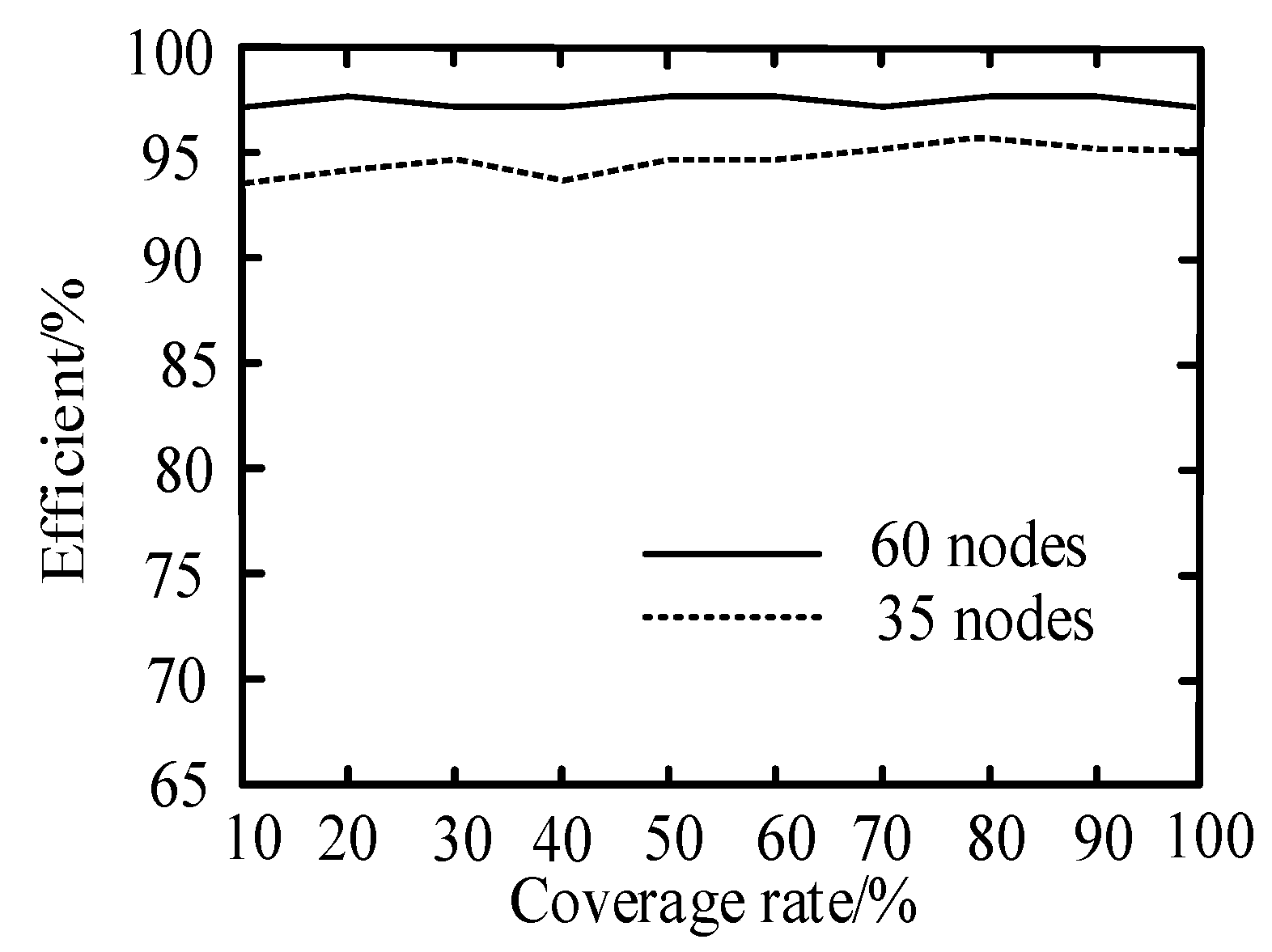
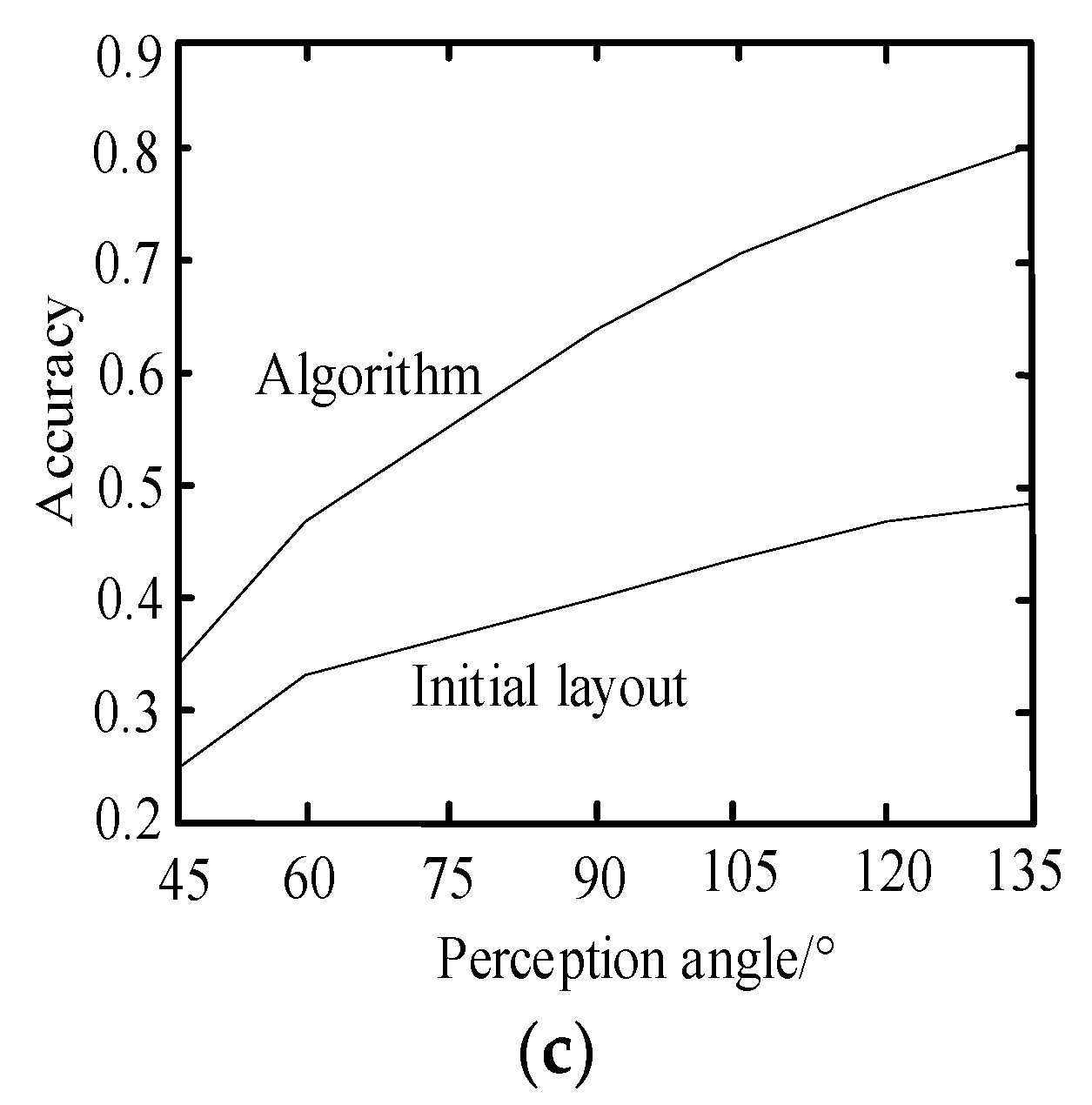
4.1.2. Influence of Parameters on the Monitoring Algorithm

According to the different number of nodes, sensing radii and perception angles, the algorithm was simulated. After monitoring the force point, the influence of index on the monitoring accuracy was discussed. The experimental results are shown in Figure 5.

Experimental results show that the accuracy is more sensitive to the changes of the node parameter, and the accuracy increases gradually with the change of parameter from small to large. When the parameters increase to a certain extent, the slope of the curve becomes smaller; that is to say, the increase degree of monitoring accuracy rate becomes smaller. The increase of redundant data when the parameter increases leads to low monitoring efficiency.

4.2. Application Effect of Monitoring Algorithm

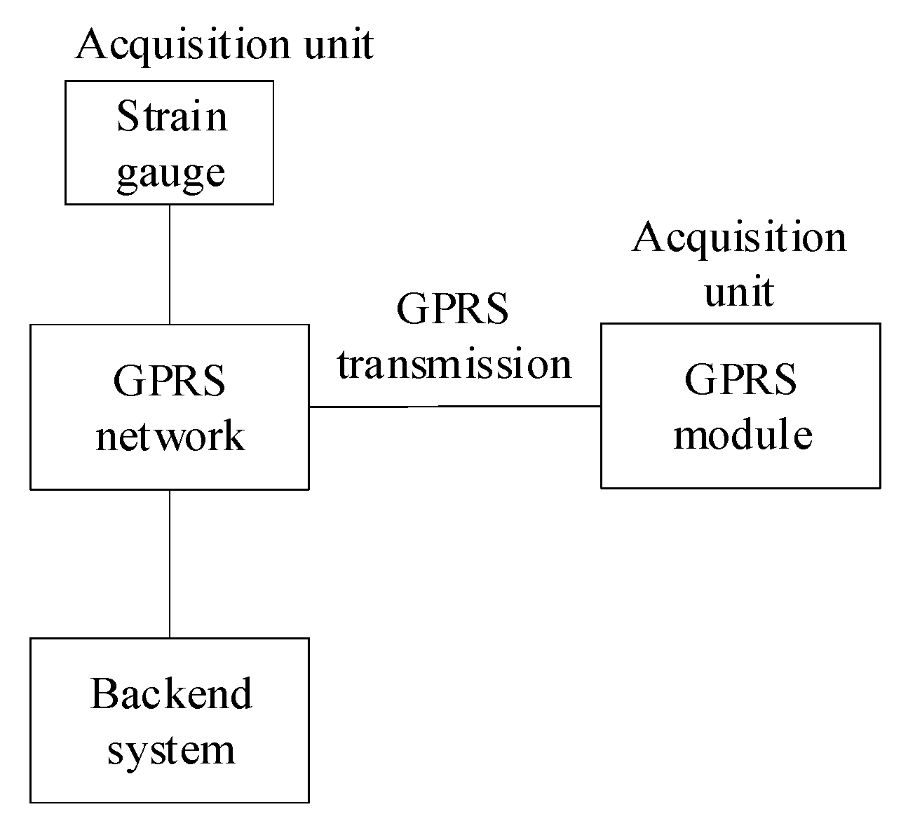
4.2.1. System Overview

In view of the installation position of the system, the problems about waterproofing and power consumption must be considered. Therefore, the wireless sensors with high measurement accuracy, good reliability and low power consumption were adopted to construct the system framework, which is shown in Figure 6. The system uses CDMA/GPRS (Code Division Multiple Access/General Packet Radio Service) as the communication mode and transmits the front-end data to the background through the Internet. The front end is powered by solar energy.

4.2.2. Field Devices and Installation

(1) Stress measurement equipment: a vibrational chord strain gauge was used in this project. Its principle: the vibrating frequency of vibrational chord strain gauge changes with the deformation of strain gauge. The change of stress of the cylinder concrete pipe structure of large buildings will lead to the deformation of the strain gauge and the vibration frequency of vibrating string in the strain gauge. Because the vibrating string is excited by the electromagnetic coil, the vibration frequency can be measured, and then the strain of steel structure can be measured. Meanwhile, the instrument can simultaneously measure the temperature in the installation point of the strain gauge.

(2) Front-end acquisition equipment: the front-end acquisition device adopts embedded low-power temperature sensor equipment, the model is PT100, the accuracy is (0.15 + 0.002 × |t|) °C, and the main board is embedded with the CDMA module. Each device provides four interfaces and connects four strain gauges at the same time. The schematic diagram of the main board of the temperature sensor is shown in Figure 7.

The front-end acquisition device can regularly collect the strain data and the temperature of the strain gauge, and supply power to the strain gauge. Meanwhile, the front-end acquisition device communicates with the background, receives the command from the background, and sends the measurement data to the background. Generally, the transmission mode is regular, and the timing interval can be set in the background. The background can also actively request data from the front-end acquisition device temporarily. During the transmission, if it is unable to establish a connection with the background communication, the data collected by the system can be saved in the front-end acquisition equipment. After the communication connection is established with the background, the local historical data can be sent to the background. Because the system runs outdoors and uses solar energy for power supply, when the system is in the transmission interval, the system will not work. In order to save power, the system is dormant when in this state, and it will not accept any command until the next transmission time.

(3) Background software: the background software system is responsible for communicating with the front-end acquisition device on site, and storing the received data into the database for analyzing and querying. Its main functions include data acquisition, data query management, sensor configuration and system configuration.

(4) Field installation: due to the difficulty of field installation, eight strain gauges are temporarily installed in two layers. Four strain gauges in each layer are connected to the same front-end acquisition device. There are two front-end devices in the pipeline, which are numbered 40 and 95, respectively. Eight strain gauges are welded to the outside of the pipe.

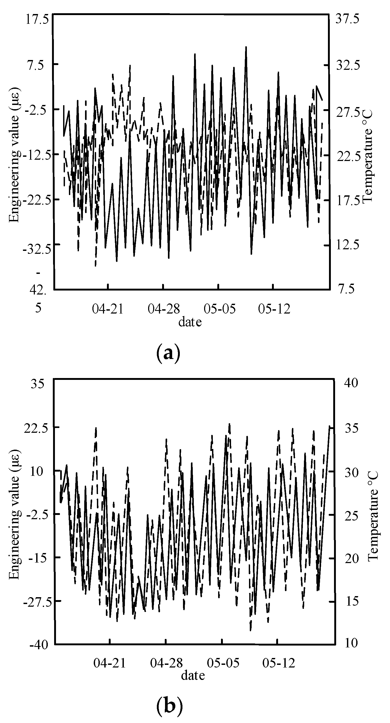
4.2.3. Real-Time Analysis of Measuring Data on the Spot

After the installation in mid-April 2019, the front-end and background of the system have been running stably without any fault. With the collection of data since 16 April 2019, some measured values and calculation results of eight stress gauges have been shown in Figure 8.

Two layers of sensors are installed. There are four sensors in each layer. The model of the strain sensor is csjmzx-3001, and the accuracy is ±0.5 °C. According to the reliability of the structure of concrete pipe of steel cylinder, the pipeline is regarded as a series model. Firstly, the reliability of each layer is calculated, and then the reliability of structure is calculated by the Ditlevsen method.

All the measurement values are strain, which should be converted into stress before calculation. The transformation relationship is shown as follows:

$$\mathsf{\sigma }=\mathrm{E}\mathsf{\epsilon }$$

(16)

In the above formula, $\mathrm{E}$ is the elastic modulus of steel cylinder [30]. For Q345 steel, E = 206 × 109 Pa.

Table 5. Test data.

Serial Number of Strain Gage	Numerical Reading (με)	Check 0 (με)	After Validation (με)	Stress (MPa)
40-1	−10.987	18	−28.987	−5.971
40-2	−7.178	6.5	−13.678	−2.818
40-3	−5.939	6.1	−12.039	−2.48
40-4	−27.521	−11.4	−17.121	−3.527
95-1	−51.455	−30.38	−21.075	−4.341
95-2	−17.476	−15.65	−1.826	−0.376
95-3	−37.176	−13.5	−23.676	−4.877
95-4	−5.502	−11.1	8.1	1.669

presents the data from 04:00 on 23 June 2019.

The solution value of reliability index β in the series model is:

$${\mathsf{\beta }}_1=6.781,{\mathsf{\beta }}_2=6.811$$

(17)

Because the measured value is not in special conditions, the reliability index β is very large. According to the normal distribution table, when the reliability index β > 4.5, the failure probability is almost 0 [31]. Therefore, the reliability index of the system can take the minimum value:

$$\mathsf{\beta }\mathrm{s}={\mathsf{\beta }}_1=6.781$$

(18)

After calculation, the algorithm has the best detection effect.

5. Conclusions

Stability has a great impact on the life and property safety of large buildings. The wide application of concrete cylinder pipes in large buildings has great significance in the study of stress points in structure, which can ensure the safety and smooth operation of production. Therefore, we provide an algorithm for monitoring the stress points in concrete cylinder pipe structures of large buildings. The test results show that the corresponding stress is calculated by using the measured strain stress at each measurement position, and then the solution value of the reliability index is obtained. According to the calculation results, the reliability index under the research method is very large. When the reliability index is large, the failure probability is almost 0, indicating that the research method has a very ideal application effect.

The main achievements are described as follows:

(1)

According to the distribution rule of circumferential prestress produced by prestressed steel wire on the pipe core concrete, the influence of buried depth, internal water pressure, pipe wall thickness and concrete strength on the stress of cylinder concrete pipe is obtained, which lays the theoretical and data foundation for the monitoring algorithm;

(2)

By designing a series of basic assumptions, the analysis process and algorithm are simplified;

(3)

The interaction force between the node and the force point is regarded as two charged particles in the virtual potential field. The force on the node and the centroid of the sensing area were analyzed. In this way, the accuracy of the monitoring algorithm was improved;

(4)

Through the simulation of the monitoring algorithm, the influence of the number of nodes, sensing radii and sensing angles on the monitoring accuracy was analyzed, and then the index was set as the best parameter to improve the reliability of the algorithm.

References

1. Cui, G.H.; Cui, K.K.; Wu, H.M.; Zhang Y., W.; Liu, J. Reliability analysis for pressing force of prestressed concrete cylinder pipe port grinding robot. Chin. J. Eng. Des. 2018, 25, 647–654. [Google Scholar]
2. Salih, C.; Manalo, A.; Ferdous, W.; Yu, P.; Heyer, T.; Schubel, P. Behaviour of timber-alternative railway sleeper materials under five-point bending. Constr. Build. Mater. 2022, 316, 125882. [Google Scholar] [CrossRef]
3. Mohammed, A.A.; Manalo, A.; Ferdous, W.; Abousnina, R.; AlAjarmeh, O.; Vijay, P.; Benmokrane, B. Design considerations for prefabricated composite jackets for structural repair: Parametric investigation and case study. Compos. Struct. 2021, 261, 113288. [Google Scholar] [CrossRef]
4. Dou, T.S.; Cheng, B.Q.; Hu, H.; Xia, S.F.; Yang, J.X.; Zhang, Q. Prototype test study on deformation law of prestressed steel concrete pipe structure II: External pressure. J. Hydraul. Eng. 2018, 49, 207–215. [Google Scholar]
5. He, C.L.; Zeng, Z.; Ma, B.S.; Zhao, Y.H.; Zhang, H.F. Surrounding soil load model for structural restoration design of concrete pipes. Geol. Sci. Technol. Inf. 2019, 38, 269–274. [Google Scholar]
6. Sun, Y.Y.; Hu, S.W.; Xue, X.; Hu, D.X.; Wang, X.L. Analysis of negative pressure bearing capacity of prestressed concrete cylinder pipe (PCCP). Concrete 2018, 346, 23–26, 31. [Google Scholar]
7. Hu, H.; Dou, T.; Niu, F.; Zhang, H.; Su, W. Experimental, and numerical study on CFRP-lined prestressed concrete cylinder pipe under internal pressure. Eng. Struct. 2019, 190, 480–492. [Google Scholar] [CrossRef]
8. Yang, W.; Fan, Z.; Wu, F. Design of wireless sensor network based on 6LoWPAN and MQTT. GuofangKejiDaxueXuebao/J. Natl. Univ. Def. Technol. 2019, 41, 161–168. [Google Scholar]
9. Al-Nasra, M. Concrete tensile strength of hollow cubes subjected to water pressure. ACI Mater. J. 2019, 116, 151–157. [Google Scholar] [CrossRef]
10. Fomichev, P.A.; Zarutskii, A.V. Fatigue life prediction by a local stress-strain criterion for hole-containing specimens after precompression of their material. Strength Mater. 2019, 51, 193–201. [Google Scholar] [CrossRef]
11. Qu, C.; Lv, Y.; Yang, Z.; Xu, X.; Zhu, D.; Yan, S. An improved chip-thickness model for surface roughness prediction in robotic belt grinding considering the elastic state at contact wheel-workpiece interface. Int. J. Adv. Manuf. Technol. 2019, 104, 3209–3217. [Google Scholar] [CrossRef]
12. Zhong-Yong, S.; Yong-Tao, J.I. Percolation model of seepage irrigation system and optimization of buried depth of irrigation pipe. Ground Water 2018, 40, 115–117, 175. [Google Scholar]
13. Zheng, J.; Zhang, C.; Li, A. Experimental investigation on the mechanical properties of curved metallic plate dampers. Appl. Sci. 2019, 10, 269. [Google Scholar] [CrossRef] [Green Version]
14. Kovalnogov, V.N.; Simos, T.E.; Tsitouras, C. Runge-Kutta Pairs suited for sir-type epidemic models. Math. Methods Appl. Sci. 2021, 44, 5210–5216. [Google Scholar] [CrossRef]
15. Mou, B.; Bai, Y. Experimental investigation on shear behavior of steel beam-to-CFST column connections with irregular panel zone. Eng. Struct. 2018, 168, 487–504. [Google Scholar] [CrossRef]
16. Ju, B.S.; Gupta, A.; Ryu, Y. Seismic fragility of steel piping system based on pipe size, coupling type, and wall thickness. Int. J. Steel Struct. 2018, 18, 1–10. [Google Scholar] [CrossRef]
17. Alajarmeh, O.S.; Manalo, A.C.; Benmokrane, B.; Karunasena, W.; Mendis, P. Effect of spiral spacing and concrete strength on behavior of gfrp-reinforced hollow concrete columns. J. Compos. Constr. 2020, 24, 04019054. [Google Scholar] [CrossRef]
18. Khedr, A.M.; Osamy, W.; Salim, A.; Agrawal, D.P. Sensor network node scheduling for preserving coverage of wireless multimedia networks. IET Wirel. Sens. Syst. 2019, 9, 295–305. [Google Scholar]
19. Van Vugt, D.C.; Kamp, L.P.J.; Huijsmans, G.T.A. Closed-Form solutions for the trajectories of charged particles in an exponentially varying magnetostatic field. IEEE Trans. Plasma Sci. 2019, 47, 296–299. [Google Scholar] [CrossRef] [Green Version]
20. Thai, P.V.; Abe, S.; Kosugi, K.; Saito, N.; Takahashi, K.; Sasaki, T.; Kikuchi, T. Interaction and transfer of charged particles from an alternating current glow discharge in liquids: Application to silver nanoparticle synthesis. J. Appl. Phys. 2019, 125, 633–645. [Google Scholar] [CrossRef]
21. Mcnamee, C.E.; Kawakami, H. Effect of the surfactant charge and concentration on the change in the forces between two charged surfaces in surfactant solutions by a liquid flow. Langmuir 2020, 36, 1887–1897. [Google Scholar] [CrossRef] [PubMed]
22. Medvedeva, M.A.; Simos, T.E.; Tsitouras, C. Exponential Integrators for Linear Inhomogeneous Problems. Math. Methods Appl. Sci. 2021, 44, 937–944. [Google Scholar] [CrossRef]
23. Abedini, M.; Mutalib, A.A.; Zhang, C.; Mehrmashhadi, J.; Raman, S.N.; Alipour, R.; Momeni, T.; Mussa, M.H. Large deflection behavior effect in reinforced concrete columns exposed to extreme dynamic loads. Front. Struct. Civ. Eng. 2020, 14, 532–553. [Google Scholar] [CrossRef] [Green Version]
24. Zhang, C.; Abedini, M. Development of P-I model for FRP composite retrofitted RC columns subjected to high strain rate loads using LBE function. Eng. Struct. 2022, 252, 113580. [Google Scholar] [CrossRef]
25. Zhu, L.M.; Zhang, C.W.; Guan, X.M.; Uy, B.; Sun, L.; Wang, B. The multi-axial strength performance of composite structural b-c-w members subjected to shear forces. Steel Compos. Struct. 2018, 27, 75–87. [Google Scholar]
26. Zhang, W.; Tang, Z.; Yang, Y.; Wei, J.; Stanislav, P. Mixed-Mode debonding behavior between CFRP plates and concrete under fatigue loading. J. Struct. Eng. 2021, 147, 04021055. [Google Scholar] [CrossRef]
27. Luo, Y.; Zheng, H.; Zhang, H.; Liu, Y. Fatigue reliability evaluation of aging prestressed concrete bridge accounting for stochastic traffic loading and resistance degradation. Adv. Struct. Eng. 2021, 24, 3021–3029. [Google Scholar] [CrossRef]
28. Rahman, A.; Oldford, R.W. Euclidean distance matrix completion and point configurations from the minimal spanning tree. Siam J. Optim. 2018, 28, 528–550. [Google Scholar] [CrossRef] [Green Version]
29. Ding, J.; Ke, Y.; Cheng, L.; Zheng, C.; Li, X. Joint estimation of binaural distance and azimuth by exploiting deep neural networks. J. Acoust. Soc. Am. 2020, 147, 2625–2635. [Google Scholar] [CrossRef]
30. Yamamoto, T.; Hanabusa, M.; Kimura, S.; Momoi, Y.; Hayakawa, T. Changes in polymerization stress and elastic modulus of bulk-fill resin composites for 24 hours after irradiation. Dent. Mater. J. 2018, 37, 87–94. [Google Scholar] [CrossRef] [Green Version]
31. Hamasha, M.M.; Al-Rabayah, M.; Aqlan, F. Standard tables of truncated standard normal distribution using a new summarizing method. Mil. Oper. Res. 2018, 15, 216–247. [Google Scholar]
Figure 1. Node sensing model.
Symmetry 14 01261 g001
Figure 2. Virtual potential field force between particles.
Symmetry 14 01261 g002
Figure 3. Stress point monitoring.
Symmetry 14 01261 g003
Figure 4. Relationship between network coverage rate and monitoring efficiency.
Symmetry 14 01261 g004
Figure 5. Relationship curve between each index and monitoring accuracy, (a): Influence of the number of nodes on accuracy (r = 3; 2θ = π/2; n = 30, 45, 60, 75, 90, 105), (b): Influence of perception radius on accuracy (n = 40; 2θ = π/2; r = 1, 2, 3, 4, 5, 6), (c): Influence of perception angle on accuracy. (N = 40; r = 3; θ = π/4, π/3, π/2, 7π/12, 2π/3, 3π/4).
Symmetry 14 01261 g005aSymmetry 14 01261 g005b
Figure 6. System framework.
Symmetry 14 01261 g006
Figure 7. Physical drawing of main board connected to temperature sensor.
Symmetry 14 01261 g007
Figure 8. Curve of count value of stress, (a): The measured value of 40−1 point, (b) The measured value of 95−3 point.
Symmetry 14 01261 g008