Position Prediction in Space System for Vehicles Using Artificial Intelligence

Abstract

This paper deals with the prediction of the future location of vehicles, which is attracting attention in the era of the fourth industrial revolution and is required in various fields, such as autonomous vehicles and smart city traffic management systems. Currently, vehicle traffic prediction models and accident prediction models are being tested in various places, and considerable progress is being made. However, there are always errors in positioning when using wireless sensors due to various variables, such as the appearance of various substances (water, metal) that occur in the space where radio waves exist. There have been various attempts to reduce the positioning error in such an Internet of Things environment, but there is no definitive method with confirmed performance. Of course, location prediction is also not accurate. In particular, since a vehicle moves rapidly in space, it is increasingly affected by changes in the environment. Firstly, it was necessary to develop a spatial positioning algorithm that can improve the positioning accuracy. Secondly, for the data generated by the positioning algorithm, a machine learning method suitable for position prediction was developed. Based on the above two developed algorithms, through experiments, we found a means to reduce the error of positioning through radio waves and to increase the accuracy of positioning. We started with the idea of changing the positioning space itself from a three-dimensional space into a two-dimensional one. With changes in the time and space of radio wave measurement, the location was measured by transforming the spatial dimension to cope with environmental changes. This is a technology that predicts a location through machine learning on time series data using a direction angle classification technique. An experiment was conducted to verify the performance of the proposed technology. As a result, the accuracy of positioning was improved, and the accuracy of location prediction increased in proportion to the learning time. It was possible to confirm the prediction accuracy increase of up to 80% with changes. Considering that the accuracy result for location prediction presented by other researchers is 70%, through this study, the result was improved by 10% compared to the existing vehicle location prediction accuracy. In conclusion, this paper presents a positioning algorithm and machine learning methodology for vehicle positioning. By proving its usefulness through experiments, this study provides other researchers with a new definition of space for predicting the location of a vehicle, and a machine learning method using direction angles.

1. Introduction

As we enter the era of the fourth industrial revolution, various fields related to automobiles, such as autonomous vehicles and smart city traffic management systems, require technology to predict the future location of vehicles. Now, anyone can easily obtain the current location of a vehicle in real time through a GPS (global positioning system). Currently, vehicle traffic prediction models and accident prediction models are being tested in various places, and significant progress has been made. However, there are still few systems that have been proven effective in predicting the future location of a vehicle, and few algorithms that have been validated when managing the location prediction of the vehicle itself from a third-party perspective. To solve this problem, we propose a location determination algorithm to improve the location accuracy and a machine learning method specialized for location data. The proposed method involves the selection of an optimal reference point that can maximize the positioning accuracy, useful for building a location prediction system for a vehicle, and a dimensional transformation location that is adaptive to changes in the environment of radio waves to predict the distance between the selected reference point and a location tracking terminal. It is a measurement method. The proposed algorithm is an algorithm that uses machine learning to output the predicted position of the vehicle in the future by using the past positioning data for the vehicle on the road as the learning data. This algorithm is based on the idea of transforming a three-dimensional space itself into two dimensions. Therefore, in this paper, with changes in the time and space of radio wave measurement, we develop a technology to measure the position by transforming the spatial dimension; this method can cope with environmental changes and predict the position through machine learning. The proposed algorithm is a new location prediction algorithm that has not been previously proposed. To verify the proposed algorithm, we check whether the positioning algorithm and the machine learning methodology for location prediction are accurately designed through experiments. As an experimental method for verification, a beacon is attached to a vehicle-type toy and placed on the grid map and toy rail, and location data are collected using the toy’s Bluetooth signal. Machine learning is used to predict the future position of a vehicle-shaped toy, and it seeks to validate the accuracy of the algorithm by showing how accurately the prediction was made.

2. Related Works

In general, a vehicle can be equipped with various positioning terminals. A representative one is the lane determination system, and it uses a wireless communication channel composed of DGPS (differential global positioning system) receivers to display the real-time vehicle position and position at the lane level through a lane matching algorithm [1]. In addition, even in the case of an intelligent transportation system that manages traffic by locating the relative positions between vehicles, it is necessary to know the latest location data of the surrounding vehicles. A vehicle location algorithm is used to determine the location of the vehicles [2]. With a stable power supply, a communication terminal can be mounted, and hence various types of positioning devices can be installed. A positioning terminal [3] has an RF low-signal transmitter, which accommodates up to 32 channels, with a time division multiplexing technique for vehicle location search, and contains more than 1500 synchronized units for unidirectional data transmission in order to report the location with multiplexing slots for time series data. It is used to collect and display data used for locating the position. In the case of a robot operated underwater rather than on the ground, the position information of the robot is acquired based on the distance of the robot, which emits a signal for positioning, and it receives the signal. However, due to the attenuation and distortion of the radio wave signal in the water, it is impossible to locate the position normally underwater, and the characteristic value of the physical position on the Earth is mainly used [4]. Of course, this technique seeks to minimize the position error by additionally capturing the trajectory of the position measurement values for the radio waves between one another for positioning in reality. However, there is a drawback: positioning can be performed only when a special terminal is installed or stable power can be supplied at all times. We believe that a suitable solution would be to determine the location without a special power supply and predict the location using the location data. Most of the outdoor positioning systems, in which existing vehicles rely on GPS, essentially have an error range of 10 m or more [5]. Nowadays, in addition to GPS, the most widely used location positioning technology is a location positioning system using WIFI or BEACON using trigonometry in the IEEE 802.15.4 wireless personal area network (PAN) environment. It uses RSS (received signal strength). However, the RSS-based positioning technology brings more positioning errors due to battery problems, water or metal existing in the surrounding environment and the influence of various radio waves. Therefore, in this paper, in order to establish a position prediction system for a vehicle, a technique for selecting an optimal reference point that can maximize the positioning accuracy, and a dimensional transformation that is adaptive to changes in the environment of radio waves to predict the distance between the selected reference point and the location tracking terminal, we propose a positioning technique. First of all, in positioning, it is very important to ensure that the error range does not exceed the reference point for the identification of the position and hence does not limit the positioning accuracy. Therefore, in order to build a position prediction system for a vehicle, it is first necessary to develop a positioning algorithm that can accurately find the position of a target vehicle in three-dimensional space. We then convert the 3D object position on a wireless PAN into a 2D one to train the prediction of the object position [5]. As a location positioning method using PAN, this method focuses on an RF-based system using trigonometry, and uses RSS as a unit of signal measurement. Issues that may arise in such a system include the method of selecting three optimal reference APs for applying trigonometry when three or more APs exist around the terminal, and predicting the distance between the selected three reference APs and the terminal. In particular, if the three reference APs are incorrectly selected, the location accuracy of the terminal predicted based on this also deteriorates. Therefore, the optimal AP selection is one of the most basic factors for improving the location positioning accuracy. The current commercial positioning algorithm using general radio waves has an inevitable error in three-dimensional space. The Doppler equation is useful when the wave velocity is much larger than the relative velocity of the wave source and the observer, when the wave source and the observer are very slow compared to the velocity of the radio wave or when the distance between the wave source and the observer is very large compared to the wavelength. If this is not the case, the Doppler equations contain a number of errors in positioning. In order to predict the distance between the terminal and the AP when a reference AP is given, there are various path loss models generally having the following equation [5]. However, when using such a path loss model, which changes the parameter values according to time and space, predicting the distance between the terminal and the AP reduces the positioning accuracy. In particular, expressing the value existing in the three-dimensional space in a two-dimensional formula inevitably involves errors. Therefore, a two-dimensional position prediction technique that can adaptably cope with environmental changes, even if the three-dimensional propagation measurement time and space change, is required for the positioning crisis method. In order to create a location prediction system using machine learning, it is necessary to propose a method to improve the position accuracy of the positioning algorithm currently being used and to develop an application algorithm for machine learning that can convert the position data into a more accurate prediction value. Our algorithm converts the location-determining object position in the 3D space into 2D, which is used to predict the object position in 3D, which best matches the original object position in 3D. In order to derive the prediction value of a mobile radio medium based on a wireless sensor network (WSN), machine learning has already been applied [6]. In the case of a system to predict the future path of the surrounding vehicle using deep learning technology such as RNN or CNN when generating location prediction data, there is a prediction model that operates in real time by recognizing the surrounding vehicles using sensors in the road environment and inputting their past paths [7]. This deep learning technique learns the model using various data, so it can show good prediction performance in various environments, and has the advantage of being simple to apply or design. Among them, the RNN method is widely used in the field of analyzing sequential data, such as in speech recognition, translation, word completion, etc. Therefore, a method has been proposed that obtains the location information of surrounding vehicles through sensor processing, and predicts how they will change in the future using RNN. For this, the authors input the velocity and yaw rate of the vehicle, camera image and the location and speed of the surrounding vehicle into an LSTM, which is a structure of RNN, and trained the LSTM to predict the future state of this information [7]. In the railway network, a radio frequency identification (RFID) technology using the location of the intersection of the vehicle switch and the railway network was used [8]. System geometry, range and azimuth information were used when estimating a target using a GPS (global positioning system) and locating the target in space using azimuth. Both synthetic and real radar data were used [9]. LiDAR positioning, one of the positioning methods, is a method based on artificial landmarks that is widely used in the warehouse logistics industry. Moreover, the existing LiDAR positioning method based on artificial landmarks mainly relies on the three-point positioning method, and its performance falls short [10]. Although structured roads are places where there are many interactions between vehicles, it is difficult to perform prediction using vehicle interactions because of the high uncertainty of movement. Thus, the future behavior of a vehicle is predicted by a subnetwork consisting of fully connected layers. Therefore, time series data can have the most reliability in predicting the future location of a vehicle [11]. Satellite navigation is useful for planning and tracking travel. The vehicle’s destination can be predicted using the time series data of the vehicle to which it has access. Where possible, it could be used for the early warning of potential hazards, bypassing routes to avoid traffic congestion and optimizing fuel consumption for hybrid vehicles. The most efficient prediction of the vehicle’s future location is based on the vehicle’s travel history [12]. Dimension reduction sparse reconstruction (DRSR) is mainly used for the problem of movement direction in two dimensions after transforming the dimension of space into two dimensions, and the method of spatial spectral reconstruction (SSRSD) is used. By using the angle decoupling method, the two-dimensional estimate is converted into two independent one-dimensional estimates, which in turn reduces the computational complexity [13]. Nowadays, the trend of the IoT environment is to achieve the convergence of artificial intelligence and sensor network. A recent trend in the research on artificial intelligence technology CNN (convolutional neural network), a method based on two-way long-term fusion [14] and wireless sensor network (WSN), is a factor for transmitting data from a mobile sensor node to a base station [15], and Smart cars generally have many sensors and microcomputers that allow the driver to obtain more information about their trip [16]. This provide with an implementation of artificial intelligence for classification [17]. It is updated, managed and monitored using a wireless sensing element network [18]. Wireless sensor networks can be integrated with thousands of small nodes, which can effectively detect, communicate and calculate parameters [19]. With the evolution of 5G wireless networks, the Internet of Things has become an innovative technology that enables various functions and applications [20]. Wireless sensor networks are the cornerstone of the current Internet of Things era, have limited resources and functions, and have smaller packet sizes than other types of networks [21]. In conclusion, the method of reducing the azimuth, which is likely to move, as a vehicle position prediction method may be the most effective. The proposed method analyzes location and speed data from the past, and predicts changes in future situations comprehensively by using camera images, roads and environmental information. In other words, a position prediction method is not used based on dynamics or motion models for the vehicle itself, since there are too many data that change in real time in a dynamics model or motion model, and it is difficult to find appropriate model parameters for actual data in 3D; moreover, in a complex environment, this is complicated and difficult to implement in real time due to the high calculation demands. However, if the environment is converted into two dimensions, the problem of positioning error can be simplified. In this paper, we first convert the real 3D space into 2D space and assume that there is a location tracking terminal in 2D space. We consider the frequency generator as a sensor using a frequency generator constituting a two-dimensional positioning terminal, and we combine an algorithm for frequency data from the positioning device and an algorithm for machine learning for data derived from the positioning technology. Therefore, we utilize the position values of the sensor received from the physical sensor to convert the data into tagged data; finally, we use technology to apply the converted data to the future prediction of the sensor’s possible location. After the verification of the performance of this technique, it can be concluded that the accuracy of the location prediction is reliable. The method that evaluates the accuracy of the prediction model uses both learning data and test data. The learning data are used to estimate the parameters of the prediction technique, and test data are used to evaluate accuracy. This can provide reliable indicators of how well the model predicts new data because test data are not used to determine the forecast. The method to learn and test data that is most reliable is time series cross-validation, which is used to set the standard of data based on time [22]. When time series cross-validation is performed, there are test data composed of one observation. The corresponding learning data consist of only observations that occur prior to observations that constitute the test data. When we construct a prediction, we do not use future measurements. Since reliable predictions cannot be obtained from a small amount of learning data, the time series observations at the beginning are not considered test data. Therefore, time can be considered to have a real predictive value beyond a certain point of time [23]. The data collection of WSN for existing vehicles is used to estimate the data probability for each vehicle through the Markov position prediction method and the Gauss analysis method; however, it is insufficient for the application range and vehicle network mobile crowd sensing. Therefore, it is necessary to design a reasonable node selection method 24]. In general, when a positioning technique for a positioning system is used, an additional training process is required in order to obtain a radio wave environment characteristic value using the conventional fingerprinting method of three-dimensional positioning coordinates. Accordingly, the system construction and maintenance cost increases. Thus, in this paper, wireless signal data used in positioning are matched with MAP, which is converted from 3D to 2D, and the position value of the data is used to perform machine learning. It is labeled to classify and determine data according to the characteristics of time series location data.

3. Text Data Analysis of Wireless Frequency for Positioning

Our positioning algorithm consists of the following three steps: (1) collect sensor data in a three-dimensional sensor network environment; (2) convert the collected data into two-dimensional position values; (3) extract the position prediction value by narrowing the possibility of the moveable prediction direction using the two-dimensional azimuth. Where the actual vehicle exists, it was converted into 2D to change the MAP of the sensor network. The sensor is designated as a positioning target by using the frequency generated from the wave source, and the algorithm for predicting the current position and future position of the positioning target is described. BEACON, a wave source sensor, is used to verify this method in the experiment because BEACON can play the role of a wave source in three-dimensional space when placed in a specific space as a low-power RF signal generator and can easily construct an experimental environment.

In three-dimensional space, BEACON becomes a wave source from the standpoint of the scanner (smartphone, receiver), and the scanner can act as an observer. In the three-dimensional space, the location of the wave source becomes the focus of the positioning of the object between environmental variables. The main contents of this paper are to obtain a target feature by processing data from the positioning of wave sources according to the form of positioning data, to obtain the current position through machine learning and to derive the predicted position expected in the future over time. To evaluate the accuracy of the prediction model for time series data, the data are divided into two parts: learning data and test data. The parameters are used to narrow the range of possibility for the positioning object to travel by starting from the intermediate reference point based on 360° in the two-dimensional space. The predicted values are evaluated using test data and the accuracy of prediction is determined through time series cross-validation. The vehicle sensors in the three-dimensional space play the role of a wave source, and the space is changed to two dimensions; then, the frequency of the wave circle is broadcast at a constant period, and the data collection from the wave circle is started from the middle reference point based on 360° in the two-dimensional space through the scanner installed around the location prediction method. The three-dimensional space consists of several cubes. The present location data are labeled in a time series based on the three-dimensional space. The labeling method is a location determination algorithm using frequency, and it is a machine learning algorithm to implement a prediction model using the tagged data. This paper describes a method to transform output and stored data into more comprehensive forms and concepts as a prediction model through abstraction and generalization via machine learning for the design of a reasonable node selection method [24] by fusing the prediction model creation, training, learning and prediction evaluation parts; thus, we can predict the location more accurately through a hidden layer in the stored data. This realizes the recognition and reception step of wireless radio frequency generated from sensors, a 3D constellation value granting step, a conversion step for the two-dimension position value, a location variable inclusion step for the two-dimension position value, the step of storing the two-dimension location value in a database through data tagging, the step of capturing the location value through the machine learning and the step of storing in the database the location prediction value. We also include the location prediction value of the sensor as the current value confirmation step. The position prediction value of the accuracy is higher than the step of confirming the prediction accuracy of the position prediction value of the sensor, which is the last step in the generation of the wireless radio frequency generated from the first step involving the wave source and the recognition step, and the present position value is continuously outputted. Moreover, by repeating the process of using the value again, the machine learning is performed for a longer period of time and more location data are accumulated, which increases the accuracy of location prediction for wave sources. The wireless sensor network (WSN) is formed in 3D space in order to constitute the environment for the positioning of 3D space [6]. Generally, the environment can demonstrate the current position of the sensor through the scanner existing in the space. The three-dimensional spatial positioning of the sensor network is converted into two-dimensional space for data, and the learned data are provided, which become the actual three-dimensional position value again.

The actual coordinate values are finally compared with the prediction values of the location prediction data, and the prediction values of the future are selected to increase the accuracy of the location prediction. One cube, presented in Figure 1 and Figure 2, was derived from a three-dimensional cube containing a vertex value from V0 to V7, which can express the location data as shown in Figure 3. V0,V1,V2,V3,V4,V5,V6,V7 can implicate data values to V0,V1,V2,V3,V6,V7. Moreover, V0,V1,V2,V3,V6,V7, similarly to Figure 3, can be transformed into four values of position data, forming a square with V0,V1,V6,V7. These are the position data of the cube containing the sensor, among the whole cube of the three-dimensional coordinate value in which the actual sensor is located, not the actual position data. The derived vertex values of the cube, V0,V1,V6,V7, are used to display a two-dimensional coordinate value. Figure 4 shows the method for converting the three-dimensional position value into a two-dimensional position value. The position value of the three-dimensional space is transformed into the position value of the two-dimensional space through the redefinition of the cube. The transformation method is A = V0,V1,V6,V7, as shown in Figure 4, and indicates the value of A in two-dimensional coordinates. The coordinates of A are the intersection of the horizontal axis VX and the vertical axis VY, and A = V0,V1,V6,V7 can be converted into AVX and AVY. Figure 4 demonstrates the creation process of the coordinates displayed as the coordinate value of two dimensions, and V0,V1,V6,V7 of the two-dimensional coordinates can be converted into V0,V2,V6,V7. The principle of deriving this value is demonstrated by point V2, where the folding point is folded when the two-dimensional plane square with the vertex of V0,V1,V6,V7 is folded in half. The derived V0,V2,V6,V7 can produce a cube having V(0,1,2,3) and V(0,1,5,7), V(0,1,4,5) and V(0,1,6) two-dimensional faces. The generated cubes are three-dimensional cubes with a vertex of V0,V1,V2,V3,V4,V5,V6,V7, and the three-dimensional cubes are three-dimensional configuration cubes with three coordinates of width, length and height.

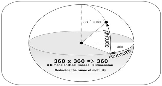
Figure 1. Altitude and azimuth of 3D space.

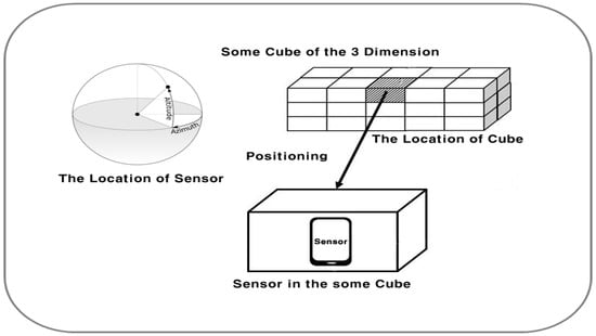
Figure 2. Definition of real 3D space.

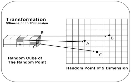
Figure 3. Converting a 3D cube to a 2D value.

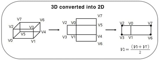
Figure 4. Converting location values.

The coordinate is included in one specific cube, including the location of sensor 1, sensor 2 and sensor 3 in the three-dimensional space, as shown in Figure 3. The three-dimensional cube with a vertex of V0,V1,V2,V3,V4,V5,V6,V7 is transformed into a two-dimensional plane value with a vertex of V0,V1,V6,V7.

The converted position value can be displayed as a coordinate at the intersection of the two-dimensional map, as a position value in a two-dimensional plane. The position values of B in two-dimensional space V0,V1,V6,V7 have the position values belonging to the cube of three-dimensional space having a vertex of V0,V1,V2,V3,V4,V5,V6,V7, as shown in Figure 4. In the three-dimensional space, the position of the vehicle can assume the cube in which the sensor exists, not the intersection point of two dimensions, as the predicted position value. This is a dimensional transformation positioning algorithm for two-dimensional and three-dimensional positioning data for the positioning of the target. The real position value of the sensor existing in 3D is converted into 2D to generate prediction data, and it is converted into actual 3D data again; moreover, the actual positioning is performed with positioning wherein the predictable position data can be easily obtained.

As shown in Figure 5, if the position of the sensor in the current 3D space has a value of A in the 2D map, the future position of the sensor can be moved to A, B or C, and the movement path must be within the baseline of the XA, XB, XC, α1, α2, α3 set based on the reference point X. Since the reference point, the reference line and the reference path are fixed, it is changed from A to B and C, which means that the future predicted position of A can be determined as one of A, B or C. The prediction model in which the location of A is changed to A, B and C in the three-dimensional space is subordinated to the reference point X, reference line XA, XB, XC and reference path α1, α2, α3. The positional movement of A in two dimensions with an azimuth of 360° is restricted to the reference point, the reference line and the reference path, so the predicted position cannot escape. The reference point, the reference line and the reference path begin from the positioning of the initial point A. When the position of A is within the first three-dimensional space, the reference point X, reference line XA, XB, XC and reference path α1, α2, α3 are automatically calculated and combined into datasets with the tagged position value for learning. The labeled position data are stored in the database automatically, in accordance with the positioning value of the current point of time of A as a time series measurement value, along with the positioning value according to the future time. The above is the positioning algorithm for the dimension-conversion sensor position prediction system using machine learning.

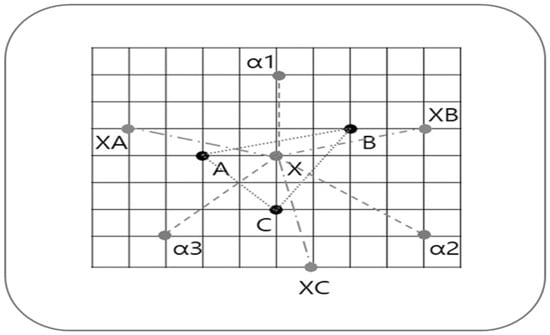
Figure 5. Movement of position value.

4. Machine Learning Methodology

This paper presents a dimension transformation positioning algorithm and machine learning methodology. The machine learning methodology involves tagging the data obtained through the positioning algorithm and implementing the learning and prediction model based on the positioning data. Assuming that the value of C is output at the greatest frequency, as in Figure 6, the value of A at the present time is the highest probability that A will move to C over time. As time passes, based on the reference point X, the position value of A is the position value of C located between XC and α3, and the position value is most likely to change. The reset baseline XA, XB and XC values can be set as baselines for positioning, which can be used to predict positions in the future. Therefore, the data obtained are included in the range of α1, α2, α3, and exist within the range of the predicted value. The position data value that exists in this predictable range is the value that best approximates the future position value, and the actual position prediction value is outputted based on the current value of C.

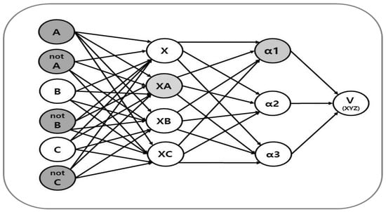
Figure 6. Learning method for predictive data.

As shown in Figure 6, the virtual position prediction value C is always dependent on XA and XC, and the time and frequency are dependent on the recognition cycle, so the position of A, derived as the current position, is inserted into the learning data, as shown in Figure 6. If the current position is A, if it is not A, if it is B, if it is C, if it is not C, if it is not C, and if it is not C, then it is not C.

The algorithm determines whether XA and a proximity relationship are formed; whether the reference point X forms a prediction and proximity relationship or not; whether XB and a proximity relationship are formed; and whether XC and a proximity relationship are formed. The virtual location, which is the reference for prediction, can be added or reduced. The current position of A will have the value of future V by relearning 1, 2, 3, which is a baseline that determines the possibility of setting the range of movement based on data obtained from X, XA, XB and XC. V can be used to derive the most likely prediction based on the measurement time. The value of V represents the coordinates of two-dimensional V0,V1,V6,V7, and can be expressed as CVX and CVY. This is converted to a position value that has a value of V0,V1,V6,V7 and refers to a three-dimensional cube with a vertex of V0,V1,V2,V3,V4,V5,V6,V7.

5. Main Equations

The forward position prediction value V of the current sensor position values A, B and C is always dependent within the azimuths of XA, XB, XC and α1, α2, α3. $\mathrm{S}=\frac{x}{360}\times \mathsf{\pi }{r}^2$ $\mathrm{l}=2\mathsf{\pi }r\times \frac{x}{360}$

$$V0,V1,V2,V3,V4,V5,V6,V7=\underset{\theta \to 0}{\lim }\frac{\sin \theta }{\theta }=1$$

(1)

$$A+B+C+XA+XB+XC+\alpha 1+\alpha 2+\alpha 3=\underset{\theta \to 0}{\lim }\frac{\sin \theta }{\theta }=1$$

(2)

The current sensor position considers the current value of A, B or C according to whether a proximity relationship is formed with any of XA, XB or XC, and whether a proximity relationship is formed with either α1, α2 or α3.

$$V0,V1,V2,V3,V4,V5,V6,V7<2\mathsf{\pi }r\times \frac{x}{360}$$

(3)

The future sensor position is determined through the pattern recognition of time series data of edge computing, and the criteria are determined according to Equations (1)–(3) above; the final future position prediction value is output as V. Therefore, the prediction position data are expressed as V(XYZ), having a 3D coordinate azimuth. Assuming that the current position value of the sensor position A is changed to the position value of C after a specific time, the position prediction value of A at the present time is V(XYZ). In conclusion, in this paper, we convert three-dimensional space into two-dimensional space and then output the data again as the positioning value of three-dimensional space. The present proposal can calculate future predictable position data based on existing learned positioning data by labeling the derived position data according to attributes and applying a learning method suitable for the characteristics of the position data to the tagging data.

6. Implementation

To verify the position prediction algorithm using machine learning through experiments, virtual vehicle model toys, assumed as vehicles on the road, are positioned and moved in MAP indicating the position scale and RAIL above them. The Bluetooth signal from the BEACON attached to the vehicle is then collected. Next, machine learning is performed using the Bluetooth data. In this way, we predict the future location of the vehicle model toy and verify how accurately it is predicted.

The order of the experiment was assumed to be a vehicle model toy with a beacon to collect radio frequency. RF data from the vehicle were collected through a scanner installed at the experimental site. The beacon was attached to the vehicle model toys and the vehicle model toys were placed on a grid map and toy rail as shown in Figure 7. The three points A, B and C based on the current position were used to prove the developed dimensional transformation positioning algorithm, and we set the reference point X in the middle. Assuming that the first A-placed vehicle is at the baseline X, A, B, C and X, XA, XB and XC, which are likely to move in the future, were displayed on the map. The vehicle model toys are displayed on the base point X, indicating the assumptions that they will be located in three places, A, B and C, and the home point when the vehicle model toy moves between A and B around the reference point X is XA. The starting point situated where the vehicle toy moves between B and C is XB. The starting point when the vehicle toy moves between C and A is XC. The above is indicated by the word on the map. After assuming XA, XB and XC around the reference point X, the azimuthal angle of the reference line in which the vehicle model toy is likely to move is narrowed. When the home position is moved between α3, XA and XB to indicate the expected position value, the home position is indicated by α2 as a word on the map, when the home position is moved between α1, XB and XC. The center axis of the reference point is placed on the map for all directions and points expected based on the vehicle model toys attached with beacons and the direction angle with the possibility of moving at 360°, and the position data are measured through the scale of the map. The expected position of B and C is assumed based on the position of the vehicle model toy A, and then the intermediate point between A, B and C is assumed as the reference point X, and XA, XB and XC home are based on X. α1, α2 and α3 are assumed based on XA, XB and XC.

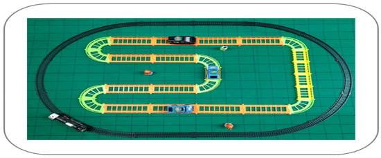
Figure 7. Grid map and toy rail used for experiment.

The vehicle model toys located at the first A point can determine through positioning data how the location changes according to time based on A, B and C. The RF from the beacon is broadcast 20 times per second, so the data scan cycle in the scanner installed within a radius of 10M is set at 0.05 s. The position data are collected based on the points of A, B and C, and the positioning data are collected after they are automatically moved by the operation of the vehicle model toys according to time; the three vehicle models and one train repeatedly pass through the same position over time, and this is used as time series test data to evaluate the performance of learning data. The experiment is performed with a beacon and scanner, and the standard of radio frequency. In order to acquire the location data of RF in the space, we produce an application for the purpose of acquiring RF data by parsing, and through this application, we obtain Txpower, major, minor and battery status information, and obtain basic information for positioning. Figure 8 presents a screen that collects RF data for positioning broadcast using the application produced. The process of collecting datasets for machine learning is to collect data, to designate the attribute type of the data, to process the ideals issued when collecting the data and to store and replace the lost data. To acquire learning data for the prediction system, the data are processed in a time series format, and the criteria are classified into seconds, minutes and time units. Datasets for machine learning are constructed by generating metadata.

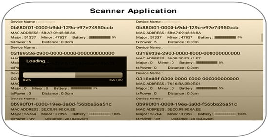
Figure 8. Scanning data of application.

The raw data extracted using the dimensional transformation positioning algorithm are labeled on each piece of data to perform machine learning, processed in time series form through annotation work and finally compiled into a CSV-type dataset for machine learning by checking the given labeling and data quality. Figure 9 presents a dataset before processing. Since data of the same form as the input data are outputted as shown in Figure 10, the methodology of this paper is proven to be accurately implemented in the wireless sensor network. The position prediction algorithm using machine learning for vehicles seeks to derive an improved position prediction value compared to the wireless sensor network, which is achieved.

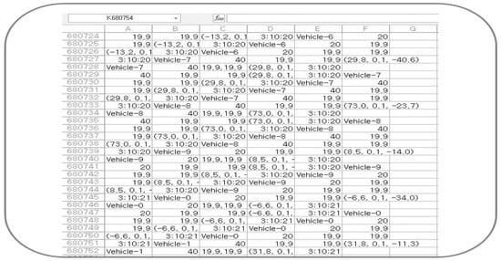
Figure 9. Dataset before processing.

Figure 10. Detailed dataset after machine learning.

The method to select the optimal reference point to maximize the accuracy of spatial positioning and a dimensional transformation positioning method to construct spatial information adaptive to changes in the propagation environment for distance prediction between the selected reference point and the terminal have been described. Based on the dimensional transformation positioning method, the goal to implement the prediction system through machine learning was verified through experiments.

7. Performance Evaluation

This paper describes the result of deriving the position of A in the future, V, by processing the data collected through the dimension transformation positioning algorithm, inputting the data set and narrowing the range within 360°—the maximum directional angle capable of moving two dimensions through the baselines. Generally, when positioning is performed, the method for predicting the location by predicting the path in the future through a search for the existing path is used [25]. It depends on the criteria, and the method of using the vehicle of the train, and the track interaction data or the dynamic response data of the vehicle regarding the shape of the track, is a typical example. In addition, a method for designing a GPS positioning object dynamically as a prediction model and regenerating all parameters while reducing execution time is proposed to obtain the location prediction data of a vehicle [26]. A vehicle travel time prediction algorithm based on past data and sharing has also been proposed [27]. A method for integrating and predicting vehicle location information such as digital map data and traffic knowledge by rough set theory was also presented [28]. The method [29] was also proposed to use the most likely vehicle path, direction change, vehicle speed and road network topology using the total travel distance after confirming the path between the start point and the end point using the vehicle location, direction, speed and road network information and the azimuth distance MAP using GPS. The present paper also proposes a vehicle location prediction method by improving the state space approach based on the geographic location of the surrounding vehicles by improving the intelligent traffic system and the intelligent road system mounted on the vehicle [30]. However, this paper describes a design for a reliable position prediction algorithm and machine learning methodology through dimension transformation of space in a wireless sensor network (WSN) [6], which differs from other existing methods. The experiment verifies the learning algorithm for prediction by narrowing the range of the dimensional transformation positioning algorithm and ultimately the start and final position within the azimuth of 360° in two dimensions. In the WSN [6], we implemented a vehicle model toy on MAP, collected location data using RF from the vehicle model toy and adopted machine learning using the location data to predict the future location of the vehicle model toy, further examining the accuracy of the prediction.

As shown in the graph of Figure 11, the output dataset was outputted within approximately 50 min, whereas the learning time was determined based on 70 min compared to the input dataset as a verification result. Predictive accuracy changed from 40% to 75%, and then dropped to 43%, rose to 74%, dropped to 51% and then rose to 80% after outputting the graph. Forecast accuracy of 40%, 43%, 51% shows a gradually rising curve according to the amount of learning time and learning data. The reason for this appears to be that the amount of learning data, which is small, and the accuracy of location prediction gradually increases as the amount of learning time and learning data increases. The position prediction data using machine learning in the wireless sensor network (WSN) [6] showed a result in which the position prediction accuracy increased according to the accumulated learning time. Therefore, it can be seen that the position prediction system using the data of the sensor can achieve higher accuracy in proportion to the optimization of the positioning algorithm and the learning time. The results of this study are expressed in a frequency waveform graph, which displays the maximum and the minimum values at the same time according to learning time, rising slowly to a certain point, as with most other location prediction systems. In addition, it is found that the learning time, the amount of learning data and the learning algorithms have a simultaneous effect, which is also related to the ratio and quality of learning data and test data.

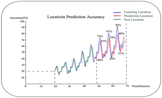
Figure 11. Predictive accuracy of position prediction.

8. Conclusions

When using a positioning technique, an additional training process is required in order to obtain a radio wave environment characteristic value using the conventional fingerprinting method of three-dimensional positioning coordinates.

The system construction and maintenance cost increases.

The proposed technique to solve this problem is the online RSS measurement technique.

RSS measurement technique is difficult to apply in 3D real space.

We propose a position prediction system by arbitrarily replacing a three-dimensional position value with a two-dimensional position value and then applying a machine learning technique to the measured position values.

In the existing positioning method, the location is determined by targeting the three-dimensional space, which is the space where the vehicle actually exists. This method inevitably entails unavoidable errors. This study presents a method for identifying a location and deriving a predicted value by using a location positioning method that predicts the distance between a terminal and an access point using a path loss model, in which the parameter values change according to time and space, which has been proposed previously, or a method using surrounding environment variables. This is a new type of positioning algorithm. We propose a method for displaying the RSS measurement value of frequency and the positional accuracy according to the signal strength of the 2D coordinate value in proportion to time using Regression, Classification, Clustering.

This study began with the idea of changing the 3D space itself into 2D in the localization space. Even when the time and space of radio wave measurement changed, the location was measured by transforming the spatial dimension to cope with environmental changes. This is a technology that predicts a location through machine learning on time series data using a direction angle classification technique. The proposed location prediction algorithm is a method for expressing a position value in a three-dimensional space as a two-dimensional data value, and extracting prediction data based on this. This is a technique for obtaining a position by transforming a spatial dimension that can adaptively cope with environmental changes, even if the time and space of radio wave measurement change, and also predicting the position through machine learning. To verify the performance of the proposed algorithm through experiments, a dimensional transformation positioning algorithm and a learning algorithm that ultimately narrows the range of the starting position and the final position within a two-dimensional 360° direction angle were verified. We collected location data using RF, predicted the future location through machine learning using the location data and verified the accuracy of the prediction. The test data for verification are the actual location derived from the existing positioning method. The research result produced in this way provides a location prediction value with 10% improvement in accuracy compared to the conventional method.

Through this study, when the location prediction algorithm and location-specific learning algorithm were applied, the accuracy of the predicted location increased by 10% compared to a previous study, in proportion to the amount of time and learning, similarly to other quantitative data. However, it is expected that a longer period of time for learning data and a greater amount of learning are required to achieve the maximum accuracy of the position prediction system when the learning time and the size of the learning data for time series location data are at the maximum. In positioning technology, it is possible to reduce errors by changing the space and to obtain a positioning system with higher accuracy through machine learning using orientation angles.

References

- Du, J.; Barth, M.J. Next-Generation Automated Vehicle Location Systems: Positioning at the Lane Level. IEEE Trans. Intell. Transp. Syst. 2008, 9, 48–57. [Google Scholar] [CrossRef]
- Ansari, K. Cooperative Position Prediction: Beyond Vehicle-to-Vehicle Relative Positioning. IEEE Trans. Intell. Transp. Syst. 2020, 21, 1121–1130. [Google Scholar] [CrossRef]
- Banks, K.M. DATATRAK automatic vehicle location and position reporting system. In Proceedings of the Conference Record of Papers Presented at the First Vehicle Navigation and Information Systems Conference (VNIS ’89), Toronto, ON, Canada, 11–13 September 1989; pp. 214–218. [Google Scholar] [CrossRef]
- Bahr, A.; Leonard, J.J.; Martinoli, A. Dynamic positioning of beacon vehicles for cooperative underwater navigation. In Proceedings of the 2012 IEEE/RSJ International Conference on Intelligent Robots and Systems, Algarve, Portugal, 7–12 October 2012; pp. 3760–3767. [Google Scholar] [CrossRef]
- Singh, A.; Shreshthi, Y.; Waghchoure, N.; Wakchaure, A. Indoor Navigation System Using Bluetooth Low Energy Beacons. In Proceedings of the 2018 Fourth International Conference on Computing Communication Control and Automation (ICCUBEA), Pune, India, 16–18 August 2018; pp. 1–5. [Google Scholar] [CrossRef]
- Al-Obaidy, F.; Razfar, N.; Moeini, P.; Mohammadi, F. Wireless Positioning Network Location Prediction Based on Machine Learning Techniques. In Proceedings of the 2020 IEEE Canadian Conference on Electrical and Computer Engineering (CCECE), London, ON, Canada, 30 August–2 September 2020; pp. 1–5. [Google Scholar] [CrossRef]
- Fan, X.; Guo, L.; Han, N.; Wang, Y.; Shi, J.; Yuan, Y. A Deep Learning Approach for Next Location Prediction. In Proceedings of the 2018 IEEE 22nd International Conference on Computer Supported Cooperative Work in Design ((CSCWD)), Nanjing, China, 9–11 May 2018; pp. 69–74. [Google Scholar] [CrossRef]
- Olaby, O.; Hamadache, M.; Soper, D.; Winship, P.; Dixon, R. Development of a Novel Railway Positioning System Using RFID Technology. Sensors 2022, 22, 2401. [Google Scholar] [CrossRef]
- Gomez-del-Hoyo, P.; del-Rey-Maestre, N.; Jarabo-Amores, M.-P.; Mata-Moya, D.; Benito-Ortiz, M.-d.-C. Improved 2D Ground Target Tracking in GPS-Based Passive Radar Scenarios. Sensors 2022, 22, 1724. [Google Scholar] [CrossRef] [PubMed]
- Zeng, Q.; Kan, Y.; Tao, X.; Hu, Y. LiDAR Positioning Algorithm Based on ICP and Artificial Landmarks Assistance. Sensors 2021, 21, 7141. [Google Scholar] [CrossRef]
- Li, L.; Sui, X.; Lian, J.; Yu, F.; Zhou, Y. Vehicle Interaction Behavior Prediction with Self-Attention. Sensors 2022, 22, 429. [Google Scholar] [CrossRef]
- Casabianca, P.; Zhang, Y.; Martínez-García, M.; Wan, J. Vehicle Destination Prediction Using Bidirectional LSTM with Attention Mechanism. Sensors 2021, 21, 8443. [Google Scholar] [CrossRef] [PubMed]
- Wang, X.; Mao, X.; Wang, Y.; Zhang, N.; Li, B. A Novel 2-D Coherent DOA Estimation Method Based on Dimension Reduction Sparse Reconstruction for Orthogonal Arrays. Sensors 2016, 16, 1496. [Google Scholar] [CrossRef]
- Chen, Q.; Xie, Q.; Yuan, Q.; Huang, H.; Li, Y. Research on a Real-Time Monitoring Method for the Wear State of a Tool Based on a Convolutional Bidirectional LSTM Model. Symmetry 2019, 11, 1233. [Google Scholar] [CrossRef]
- Ghaleb, M.; Subramaniam, S.; Ghaleb, S.M. An Adaptive Data Gathering Algorithm for Minimum Travel Route Planning in WSNs Based on Rendezvous Points. Symmetry 2019, 11, 1326. [Google Scholar] [CrossRef]
- Xiao, J.; Wu, H.; Li, X. Internet of Things Meets Vehicles: Sheltering In-Vehicle Network through Lightweight Machine Learning. Symmetry 2019, 11, 1388. [Google Scholar] [CrossRef]
- Chao, K.-W.; Hu, N.-Z.; Chao, Y.-C.; Su, C.-K.; Chiu, W.-H. Implementation of Artificial Intelligence for Classification of Frogs in Bioacoustics. Symmetry 2019, 11, 1454. [Google Scholar] [CrossRef]
- Kim, T.-h.; Solanki, V.S.; Baraiya, H.J.; Mitra, A.; Shah, H.; Roy, S. A Smart, Sensible Agriculture System Using the Exponential Moving Average Model. Symmetry 2020, 12, 457. [Google Scholar] [CrossRef]
- Koyuncu, H.; Tomar, G.S.; Sharma, D. A New Energy Efficient Multitier Deterministic Energy-Efficient Clustering Routing Protocol for Wireless Sensor Networks. Symmetry 2020, 12, 837. [Google Scholar] [CrossRef]
- Hassan, R.; Qamar, F.; Hasan, M.K.; Aman, A.H.M.; Ahmed, A.S. Internet of Things and Its Applications: A Comprehensive Survey. Symmetry 2020, 12, 1674. [Google Scholar] [CrossRef]
- Liu, F. Majority Decision Aggregation with Binarized Data in Wireless Sensor Networks. Symmetry 2021, 13, 1671. [Google Scholar] [CrossRef]
- Al Sonosy, O.; Rady, S.; Badr, N.L.; Hashem, M. A paper of spatial machine learning for business behavior prediction in location based social networks. In Proceedings of the 2016 11th International Conference on Computer Engineering & Systems (ICCES), Cairo, Egypt, 20–21 December 2016; pp. 266–272. [Google Scholar] [CrossRef]
- Qi, Y.; Yang, Z.; Qin, Z.; Liu, Y.; Chen, Y. Big Data Prediction in Location-Aware Wireless Caching: A Machine Learning Approach. In Proceedings of the 2019 IEEE Global Communications Conference (GLOBECOM), Waikoloa, HI, USA, 9–13 December 2019; pp. 1–6. [Google Scholar] [CrossRef]
- Yan, J.; Chen, C.; Zhang, D. Node selection method based on Markov location prediction in vehicle networking. In Proceedings of the 2018 IEEE 4th Information Technology and Mechatronics Engineering Conference (ITOEC), Chongqing, China, 14–16 December 2018; pp. 754–758. [Google Scholar] [CrossRef]
- Bonaventura, C.S.; Palese, J.W.; Zarembki, A.M. Intelligent system for real-time prediction of railway vehicle response to the interaction with track geometry. In Proceedings of the 2000 ASME/IEEE Joint Railroad Conference (Cat. No.00CH37110), Newark, NJ, USA, 6 April 2000; pp. 31–45. [Google Scholar] [CrossRef]
- Alzyout, M.; Alsmirat, M.; Al-Saleh, M.I. Automated ARIMA Model Construction for Dynamic Vehicle GPS Location Prediction. In Proceedings of the 2019 Sixth International Conference on Internet of Things: Systems, Management and Security (IOTSMS), Granada, Spain, 22–25 October 2019; pp. 380–386. [Google Scholar] [CrossRef]
- Chen, P.; Lu, Z.; Gu, J. Vehicle Travel Time Prediction Algorithm Based on Historical Data and Shared Location. In Proceedings of the 2009 Fifth International Joint Conference on INC, IMS and IDC, Seoul, Korea, 25–27 August 2009; pp. 1632–1637. [Google Scholar] [CrossRef]
- Chen, L.; Wei, S.; Shi, L. Research on location prediction of vehicular networks. In Proceedings of the 2009 2nd IEEE International Conference on Computer Science and Information Technology, Beijing, China, 8–11 August 2009; pp. 558–561. [Google Scholar] [CrossRef]
- Gong, X.; Manoharan, S. On predicting vehicle tracks. In Proceedings of the 2011 IEEE Pacific Rim Conference on Communications, Computers and Signal Processing, Victoria, BC, USA, 23–26 August 2011; pp. 31–36. [Google Scholar] [CrossRef]
- Pingsheng, L.; Xiaoli, X.; Bin, L.; Meng, W. The Model of Vehicle Position Estimation and Prediction Based on State-Space Approach. In Proceedings of the 2009 Second International Conference on Intelligent Computation Technology and Automation, Changsha, China, 10–11 October 2009; pp. 822–825. [Google Scholar] [CrossRef]
Publisher’s Note: MDPI stays neutral with regard to jurisdictional claims in published maps and institutional affiliations. |
© 2022 by the authors. Licensee MDPI, Basel, Switzerland. This article is an open access article distributed under the terms and conditions of the Creative Commons Attribution (CC BY) license (https://creativecommons.org/licenses/by/4.0/).