A Few-Shot Dental Object Detection Method Based on a Priori Knowledge Transfer

Abstract

With the continuous improvement in oral health awareness, people’s demand for oral health diagnosis has also increased. Dental object detection is a key step in automated dental diagnosis; however, because of the particularity of medical data, researchers usually cannot obtain sufficient medical data. Therefore, this study proposes a dental object detection method for small-size datasets based on teeth semantics, structural information feature extraction, and an a priori knowledge migration, called a segmentation, points, segmentation, and classification network (SPSC-NET). In the region of interest area extraction method, the SPSC-NET method converts the teeth X-ray image into an a priori knowledge information image, composed of the edges of the teeth and the semantic segmentation image; the network structure used to extract the a priori knowledge information is a symmetric structure, which then generates the key points of the object instance. Next, it uses the key points of the object instance (i.e., the dental semantic segmentation image and the dental edge image) to obtain the object instance image (i.e., the positioning of the teeth). Using 10 training images, the test precision and recall rate of the tooth object center point of the SPSC-NET method were between 99–100%. In the classification method, the SPSC-NET identified the single instance segmentation image generated by migrating the dental object area, the edge image, and the semantic segmentation image as a priori knowledge. Under the premise of using the same deep neural network classification model, the model classification with a priori knowledge was 20% more accurate than the ordinary classification methods. For the overall object detection performance indicators, the SPSC-NET’s average precision (AP) value was more than 92%, which is better than that of the transfer-based faster region-based convolutional neural network (Faster-RCNN) object detection model; moreover, its AP and mean intersection-over-union (mIOU) were 14.72% and 19.68% better than the transfer-based Faster-CNN model, respectively.

1. Introduction

With people paying more attention to their oral health, the demand for dental resources has also increased; to help doctors complete diagnoses with a lower cost and higher speed, researchers have developed many automatic and semi-automatic dental health diagnostic methods. Researchers often use Faster-RCNN [1] in dental object detection tasks, as it is more accurate than a one-stage object detection method for medical images. At present, U-Net, Faster-RCNN, and other related models are more popular in the auxiliary diagnostic detection area of dental medical images than some State-Of-The-Art (SOTA) models that use a general-purpose dataset. General-purpose object detection uses more advanced methods, such as efficientdets and you only look once (YOLO); in addition, Swin transformers and their derivatives are already at the SOTA level.

However, so far, most advanced object detection models have relied on a large number of labeled data. These methods (such as YOLO, Faster-RCNN, and Swin transformers) are excellent in the case of sufficient data, because they have a better fit with a large number of training samples. However, in the case of learning with a medical image dataset, such as panoramic dental images, data acquisition may be difficult, because of patient privacy concerns. Therefore, many advanced object detection models cannot be extended to medical data. Moreover, object detection under few-shot has gradually attracted the attention of researchers, and people have proposed some small-sample object detection methods based on meta-learning and transfer learning. However, only a few small-sample studies are available in the field of dental object detection. Therefore, an object detection method that relies on a small number of samples for dental images is proposed.

The contributions of this study are as follows:

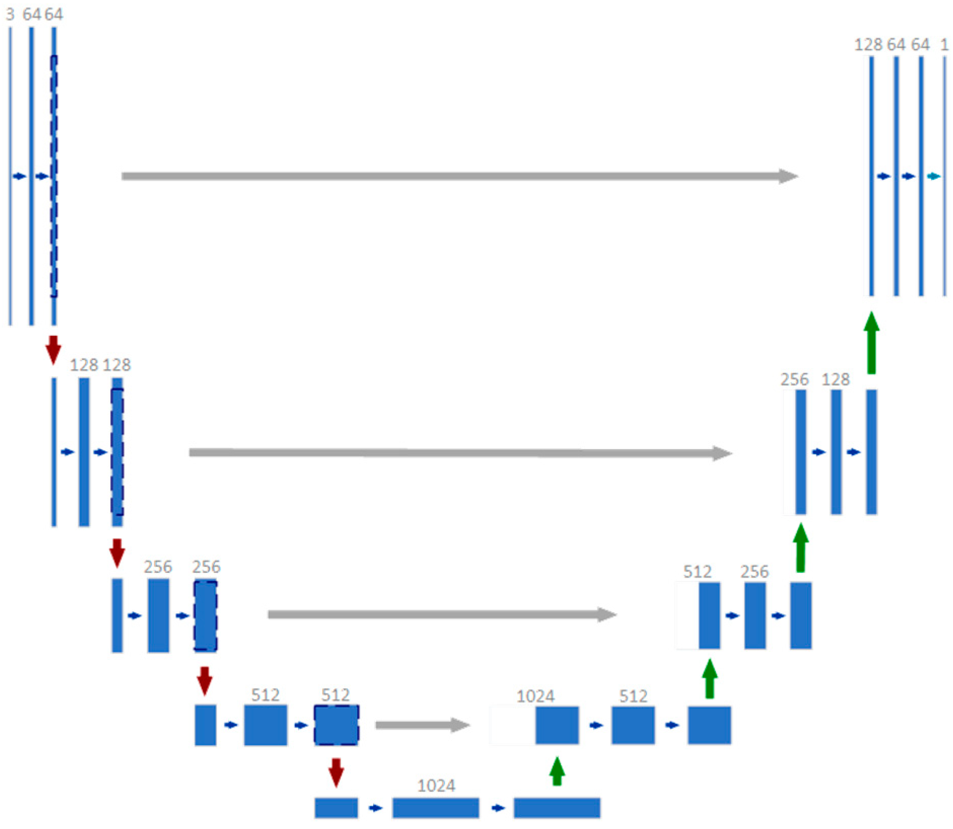
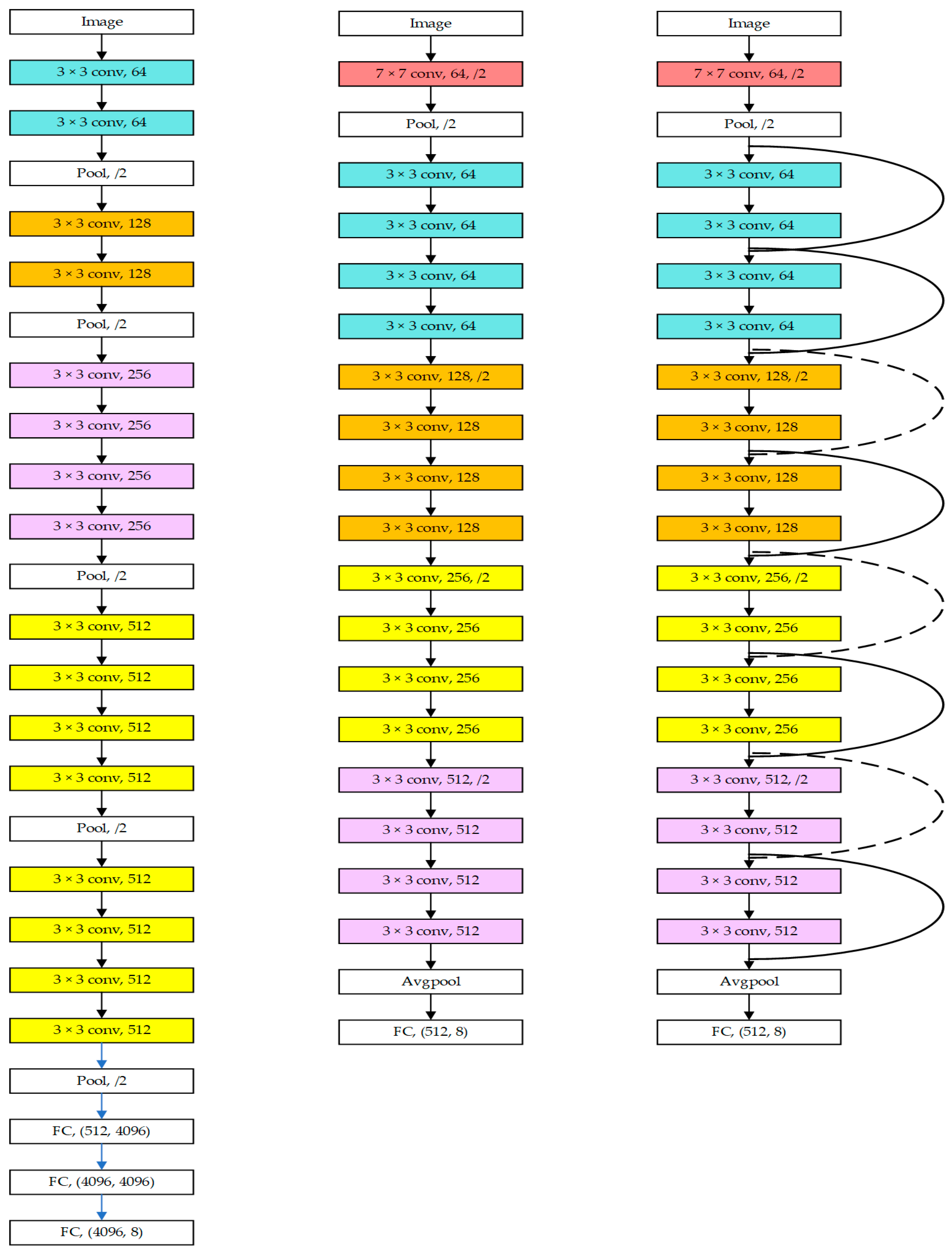
• Image segmentation technology is widely used in the field of medical image recognition, this study proposes an object detection method using dental image data, which uses a priori knowledge of dental semantics to generate a key point of the object instance. From the perspective of symmetry, in the process of generating the a priori knowledge feature map, the same structure of the network is used in the generation process of the edge and semantic feature map, and there is no master–slave relationship (as shown in Figure 1). Then, it generates a single object instance using the a priori knowledge of the object key point and the dental semantic. Compared with the direct use of a semantic segmentation model, the accuracy and recall of SPSC-NET are higher. In addition, the object detection in SPSC-NET is based on image segmentation. This technology is widely used and is a cornerstone method in the medical imaging field. Therefore, the proposed method is more suitable for dental medical images when compared to Faster-RCNN.

2.

Since the characteristic differences between each kind of tooth are relatively small, improving the classification performance of teeth in the model can significantly improve the final object detection performance. This study proposes a tooth object classification method based on structural information images. In the specific case of teeth classification, the extracted dental semantic feature information is transferred to the target domain as a priori knowledge; the feature map of the a priori knowledge is called a tooth structure information feature. With only 10 training set images, the proposed method is superior to a neural network classification method based on grayscale teeth images. In addition, this study uses information entropy compression methods to enhance the classification performance, which was proven through experiments.

Figure 1. The overall structure of SPSC-NET.

The rest of the paper is structured as follows: Section 2 reviews the application of deep neural networks (DNN) in the dental medical field and the development of small-sample object detection. Section 3 explains the proposed SPSC-NET method. Section 4 presents the experimental results and analysis, and Section 5 gives the conclusions.

2. Related Works

Tooth segmentation is an important step in the medical diagnosis of a tooth. In the study of dental images, small-sample studies on segmentation tasks are abundant. Medical images typically have the characteristics of multi-mode, small size of data, etc. Before artificial intelligence technology became popular, the diagnosis of teeth was often semi-automatic and low-level.

U-Net [2] is an automated, small-sample DNN model that automatically segments tooth structures, such as enamel, tooth body, and crown in dental X-ray images. The architecture of U-Net includes a skip path, to capture context, and a better decoding path than a fully convolutional network (FCN) [3], and the average dice similarity of all classes in U-Net is 56.4%. Subsequently, improved models based on the U-Net network have appeared [4,5,6,7], along with research on tooth segmentation based on U-Net [8,9,10]. In 2020, Gherardini et al. [11] used a transfer learning method to train a U-NET network; compared with the latest segmentation model at the time, the proposed U-NET achieved considerable performance gains, in terms of segmentation precision (0.55, 0.26, and 0.17 on three different dataset). Chen et al. [12] used a three-dimensional (3D) convolution network to obtain a single tooth in a Cone Beam CT (CBCT) image of a small-sample dataset (25 images), and realized a dice similarity coefficient of 0.936, which was similar to the results of Koch et al. [10]. Xu et al. [13] proposed dividing the teeth in 3D dental images; the upper teeth precision was 0.990 and the lower teeth division precision was 0.987. Zhao et al. [14] proposed TSASNet, a tooth panoramic X-ray image two-stage attention sematic segmentation network, to solve the problems encountered in dental boundary and dental segmentation tasks due to the low intensity distribution; and the method proposed by the authors achieves a precision of 0.9694, a Dice coefficient of 0.9272, and a recall rate of 0.9377. In 2019, KHERAIF used a deep learning and convolutional neural network (CNN) to handle the key area division of dental images [15] and showed an improved result; the precision was 97.07%.

If the processing (classification, box, stroke) for teeth (classification, box, stroke) is done manually, you need a large amount of labor and time costs, and with the application and popularity of DNN, significant progress based on computer automatic generation has helped automated dental image diagnosis. Recently, Faster-RCNN [1] and a custom architecture [16,17] was used to detect dental images. Laishram et al. [16], using the Faster-RCNN method, achieved a maximum tooth detection precision of 0.910. Leather [18] proposed a region proposal-based Faster-RCNN, which improved tooth tags used in the toothgiles. They divided 1250 images into 800, 200, and 250 for training, verification, and test samples, respectively. Their method involves two steps: first, a network is trained to identify the missing dental position; second, the Faster-RCNN is trained from the movable mark number. Their experimental results were close to the results of a human expert (98.8 and 98.5 on precision and recall). In addition, some studies on dental imaging have been related to Mask R-CNN [19]. Cui et al. [20] used Mask R-CNN to identify CBCT images of teeth with a Dice coefficient of 0.9237; Moutselos et al. [21] used the Mask R-CNN directly to detect caries, achieving precisions of 0.889, 0.778, and 0.667 in the most common, centroid pixel class, and worst classes, respectively. Mask R-CNN can be supplemented by Faster-RCNN, which is characterized by incorporating splitting functions into the Faster-RCNN, to implement instance segmentation. Jader et al. [22] increased the precision, and precision of the tooth instance segmentation, in a dental panoramic radiograph (DPR) image to 0.980 and 0.940. Although several CNN-based single-stage object detection architectures, such as YOLO [23] and single shot multibox detector (SSD) [24], have been proposed in recent years, they do not generate a region of interest (ROI) separately. However, there have been no studies on YOLO and SSD with dental image data. This may be because tooth targets are closely distributed, and the single-stage object detectors such as YOLO and SSD are inferior to Faster-RCNN in their ability to detect tooth targets.

Classifying teeth is an important task in an automated diagnostic process. Since 2017, the performance of the ImageNet benchmark has been saturated, and the use of more complex architectures has had little effect, which is not conducive to applying intelligent diagnosis technology for dental images [25]. Therefore, AlexNet [26], visual geometry group (VGG) [27], and other simple networks are still popular when analyzing dental images [28,29,30,31]. Some researchers have studied the classification task on a small sample of tooth periapical images [32,33]. Yang et al. [32] classified dental disease test F1-Sore, precision, and recall up to 0.749, 0.756, and 0.742. Zhang et al. [33] performed 33 classifications of teeth, with the F1-Sore, precision, and recall reaching 80.4, 80.3, and 80.6. Oktay [34] used an AlexNet-based CNN architecture for molar and premolar classification using 100 DPR images and achieved an accuracy of 0.943. Similarly, Miki et al. [30] used an AlexNet-based DNN model to classify teeth using CBCT images, with an accuracy of 0.888. In 2017, Le et al. [35] proposed a DDS algorithm to classify and segment teeth; when compared to the traditional method, the accuracy of DDS was 92.74%. In addition, there have been studies on extracting personal information from teeth [30,36], and these methods can infer the gender and age of patients.

An increase in the number of training samples improves the performance of models based on deep learning. According to the statistics of the review article by Singh et al. [25], in the field of tooth object detection, a maximum of 1500 tooth images were used for training, which is in the field of medical images. The medium is massive, and at least 52 images are used. In the field of medical image recognition, it is usually difficult to obtain a sufficient number of training samples. Although there are related studies on segmenting dental medical images under few-shot learning, achieving dental goals in the case of few-shot detection is a challenging task. For a few-shot object detection task, there are exactly K annotated object instances available for each class in the dataset to be detected. Therefore, few-shot object detection is referred to as K-shot detection. In the field of small-sample object detection, most of the related methods are improved versions of Faster-RCNN [37]. Small-sample object detection is divided into two types: meta-learning-based, and transfer learning-based. As a meta-learning method, Kang et al. [38] designed a one-stage small-sample detection model in 2019, which was the first research in the field of meta-object detection, and the authors reached an AP of 47.2 under the PASCAL VOC2007 10 shots dataset. In the same year, a meta-learning-based method named Meta R-CNN was proposed by Yan et al. [39]. Here, the author adopted the Faster-RCNN model and carried out meta-learning-based transformation, where Meta R-CNN implemented an AP of 51.5 in the PASCAL VOC2007 10 shots dataset. Zhu et al. [40] proposed an incremental paradigm iFSD for small-sample object detection, which defined the small-sample learning paradigm of D_base and D_novel and provided a good foundation for subsequent research; the method proposed by Zhu et al. had a population AP value of 13.7 and a total AR value of 16.5 in MSCOCO2017 10-shot. To improve the compatibility between the support set and the query set, FSDetView [41] designed a new feature aggregation module based on Meta R-CNN, and the obtained effect was better than the more famous TFA [42], which was the SOTA at that time. The concept of an attention mechanism has achieved remarkable achievements in many fields; and similarly, this idea can be applied to the field of small-sample object detection [43]. Attention-RPN [43] reached an AP value of 16.6 on the FSOD training set. On the Microsoft Common Objects in Context (COCO or MSCOCO) dataset (10-shot version), the best method for meta-learning-based small-sample object detection was DAnA-FasterRCNN [44], which solved the problem of poor matching between the features of the image to be queried and the features of the query object; the AP value of DAnA-FasterRCNN on the 10-shot MSCOCO dataset was 18.6. The process flow of methods based on transfer learning is often simple. The basic principle of a transfer learning-based method is to transfer the feature set of the source domain to the target domain and adapt it to the new task. Transfer learning is divided into four types of transfer: instance, feature, parameter, and relation-based. For parameter transfer in medical images, Akselrod-Ballin et al. [45] modified Faster-RCNN and added a classification structure to the original secondary structure. This classification structure was trained separately and transferred directly. The training samples were tailored from the object detection training set. This structure reduced the false positive rate; the method proposed by Akselrod-Ballin et al. had a measure of 0.93 on the true positive rate. Moreover, the structure was similar to the construction concept of the classifier used here, but the classification task of this method itself was only to determine whether the target was diseased, which is relatively simple. For feature-based transfer-learning, Chung et al. [46] added a priori knowledge of the tooth position to the loss function, to improve the performance of the tooth object detection model; the method proposed by Chung et al. had a measure of 0.77 on AP with 818 teeth x-ray training images, and, in addition to the tooth identification task, also obtained a 0.997 precision and 0.975 recall. The a priori information of tooth arrangement was also studied by [17,18]. These methods were infused with a priori knowledge of teeth post-processing; the method proposed by Tuzoff et al. [17] achieved a precision of about 0.9945 in detection of tooth targets, and the authors used 1352 pieces from tooth images. Regarding the influence of the third molars on the mandibular dental nerves, researchers have used the multi-level U-Net series to generate a priori knowledge and output the ideal mandibular dental nerve detection results [47]; in an experimental data test, the third molar and inferior alveolar nerve’s mean dice-coefficient reached 0.947 and 0.847; however, they did not achieve small-sample object detection for the whole mouth. Similarly, this study also used multi-level U-Net to extract a priori knowledge features of teeth. In the research on general small-sample datasets, the earliest small-sample object detection method based on transfer learning was proposed by Chen et al. [48]. To improve the generalization ability of the model in small-sample scenarios, they transferred the source domain knowledge to the target domain categories, before the second training stage; the weights of the new classes were initialized by the base class weights using the assignment of the base class similarity, which was followed by fine-tuning with the regularization of the transferred knowledge as an additional loss term, on an experimental data test; the AP value of LSTD was 38.5 for the PASCAL VOC2007 10-shot dataset. The bottom-up attention mechanism provided a priori knowledge about salient regions. Chen et al. [49] proposed a few-shot object detection (FSOD) method that combined attention mechanisms in two directions, to achieve better object bounding box generation. In terms of results, this method surpassed the existing FSOD methods at the time, the novel class’s AP value in the PASCAL VOC2007 10-shot dataset test reached 56.0. The method based on transfer learning completed the task well in the target frame selection stage, but not in the classification stage. Therefore, certain researchers believe that the key to improving the overall performance of object detection is to improve the accuracy of classification [50,51]. The proposal of TFA [42] has made transfer learning-based few-shot object detection a possibility. This method proposes using cosine similarity to improve the classification performance, and transfer learning with the use of cosine similarity improves by 2% to 20% the meta-learning approach; the novel class’s AP value in the PASCAL VOC2007 10 shots dataset test also reached 56.0. Although TFA improves the performance of the model in recognizing new classes, it does not conduct in-depth research on the a priori knowledge of the base classes. Some researchers have proposed that the key to improving the overall performance of FSOD is to improve the feature connection between the source and target domains. Some researchers combined semantic information with the source domain [52] and introduced the explicit relation feature extraction method into the learning of new object detection, to improve the ability to identify new categories; the novel class’s AP value in the PASCAL VOC2007 10 shots dataset test reached 56.8. A similar method is FSOD-UP [53], which improves the intrinsic connection between the source domain and the target domain. However, contrary to the author’s point of view in [52,53], Xu et al. [54] believed that the main threat to a classification model in judging classes lies in the shared features among classes; the AP value in the PASCAL VOC2007 10 shots dataset test reached 56.5, slightly inferior to [52,53], but the AP in the three-shots test was 49.1, ahead of previous works. In 2021, Qiao et al. [55] proposed DeFRCN, which only lagged behind DAnA-Faster-RCNN 0.1(18.5) in MSCOCO (10-shot); the novel class’s AP value in the PASCAL VOC2007 10 shots dataset test reached 60.8. Qiao studied the current small-sample object detection methods, improved the current small-sample object detection most frequently using TFA as a prototype, and innovated a multi-stage feature extraction method and classification result calibration method.

Both meta-learning-based object detection methods and transfer learning-based detection methods are based on a general object detection data set. The characteristics of panoramic dental images are inconsistent with the public general data set, and, therefore, these methods have yet to be used in the field of tooth object detection; and their performance remains to be investigated. When a doctor judges a tooth category, it is necessary to combine the position of the tooth and its morphological information. This is a kind of a priori knowledge. Dental medical image processing based on semantic segmentation can provide this a priori knowledge for classifying teeth. In this study, a small-sample object detection method based on a priori knowledge transfer is proposed. This method generates structural feature images with a priori knowledge by generating key points of tooth targets, tooth edge images, and tooth segmentation images. Then, the model can obtain the a priori knowledge information required for judging the position and category of teeth with a higher accuracy.

3. Few-Shot Teeth Detection Method-SPSC-NET

Object detection is mainly divided into two tasks: 1. generate object boxes; 2. classify each object. This section will introduce the tooth object generation method SPSC-NET under few-shot. In the first process of SPSC-NET, the semantic segmentation image of the tooth is extracted, and then the key regions in the panoramic tooth image are extracted; next U-Net is used to extract the edge information of the tooth object, using tooth semantics and edge information to extract the center point and generating a segmented image of a single tooth object. Finally, SPSC-NET classifies the teeth based on the a priori knowledge information of the teeth.

3.1. Extraction of Key Regions of Teeth Based on Semantic Information

If the original sample of the tooth image is directly put into the model for training, it will lead to a poor generalization ability of the model, owing to imbalance of the black and white pixel ratio. Figure 2 shows the performance of the trained semantic segmentation model for few-shot. It can be observed that, in addition to the segmentation ability of the teeth region, there will be some incorrect segmentation regions in the area around the teeth. In order to obtain better results for dental object detection, we need to extract the key areas of the teeth from the panoramic X-ray image of the teeth, so that the ratio of black and white pixels of the image mask will be more reasonable and exclude those areas that do not need to be identified; i.e., key areas need to be framed and cut out. The model used to extract the semantic segmentation image of teeth in this paper is U-Net, and the U-Net network structure is shown in Figure 3, which performs well in small-size datasets.

Figure 2. Key region extraction of teeth.

Figure 3. U-Net network structure.

To accurately extract the key areas of the tooth image in a small sample, this study designs a simple and reliable method that relies on two indicators: (1) the proportion of white pixels, and (2) the deviation of the longitudinal center from the longitudinal center of the sub-frame. The calculation formula for the proportion of white pixels is N_white/N_total, where N_white is the number of white pixels and N_total is the total number of pixels in the image frame. The calculation formula for the deviation value ε_offset between the longitudinal center and the longitudinal center of the sub-frame is as follows:

$${\epsilon }_{offset}={\overline{C}}_{col}-C_{absolute}$$

(1)

${\overline{C}}_{col}$ is the average of the longitudinal coordinates of the white pixels in the image frame, and $C_{absolute}$ is the absolute longitudinal center coordinate of the image frame. The difference between them is the deviation between the longitudinal center of the image and the longitudinal center of the sub-frame.

The purpose of this algorithm is to automatically extract the key areas in the panoramic dental image. The implementation method involves taking the top of the image as the starting point and the bottom center of the image as the end point, then slidingly counting the two indicators of each sliding sub-window. First, the proportion of white pixels in each image frame are sorted in descending order. The higher the proportion of white pixels, the greater is the probability that the teeth area is in the best position in the frame. Subsequently, the first 1/3 of the first sorting result is intercepted; this is because in these results, indicator 1 of the image of the individual non-key area is higher than that of indicator 1 of the image of the key area. To obtain a more accurate result, the first 1/3 of the results need to be retained, and indicator 2 is the second sorting based on the first sorting. With regards to the result of indicator 2, the data of the key area image in indicator 2 are better than the indicator 2 data value of the inaccurate key area image; therefore, the first value of the second sorting is the coordinate of the key area image.

As shown in Algorithm 1, the semantic segmentation image of teeth is used as the input, and the width and height values of key areas (w and h) are set. The height and width of the key area image are constant and only need to be defined once. The method of determining the height and width of the image in the key area is to first manually crop the training images to obtain sub-images, then calculate the average of length and width, and then round to an integer, to obtain the height and width of the automatically cropped sub-images. Before counting the values of indicators 1 and 2 of each sub-frame, it is necessary to count the weighted value of each row of pixels, avoid the increase in time complexity caused by repeated calculations, and then, start to count the two indicators of each sub-box. After the statistical analysis is completed, list L is sorted in ascending order of the reciprocal of indicator 1. Then, the first 1/3 of the sorting result is intercepted, the list L is sorted in ascending order, based on indicator 2, and the first value of the sorting result is finally obtained as the coordinate value of the upper left corner of the key area. The algorithm complexity in Algorithm 1 is O (mn²), where m is the difference between the height of the image and the height of the sub-image $H-h$, and n is the length and width of the sub-image.

Algorithm 1

INPUT: Semantic segmentation image S OUTPUT: Coordinate of Upper left and Lower right X1, Y1, X2, Y2 Parameters: Width of Sub image w      Height of Sub image h W is the width of Semantic segmentation image H is the height of Semantic segmentation image $\mathrm{L}:=\{ \}$ $A=\left\{i\ast {\displaystyle \sum }_{j=\frac{W-w}{2}}^{\frac{W+w}{2}}{S}_{j,i}\right\}for i in \left(0,H-h\right)$ $for i in \left(0,H-h\right):$    $t≔{\displaystyle {\displaystyle \sum }_{j=\frac{W-w}{2}}^{\frac{W+w}{2}}}{\displaystyle {\displaystyle \sum }_{k=i}^{i+h}}{S}_{j,k}$    $\epsilon ≔|\frac{{{\displaystyle \sum }}_{j=i}^{i+h}{A}_j}{t}-i-\frac{h}{2}|$    $L_i=\{\frac{1}{t},\epsilon ,i\}$ $L=sort(L,sort by first element \frac{1}{t})$ $L=\left\{L_i\right\} for i in (0, \frac{h}{3})$ $L=sort(L,sort by second element \epsilon )$ $X_1=\frac{W-w}{2}$ $X_2=X_1+w$ $Y_1=L_{0,2}$ $Y_2=Y_1+h$

3.2. Training Set Augmentation Method Based on Teeth Semantic Information

At a large scale, the overall arrangement and brightness of dental X-ray images from different patients vary significantly. The difference at the micro level is manifested in local characteristics. The reason for this may be because of subtle variations in the shape of the teeth of different patients. For example, the central teeth shown on the left of Figure 4a are larger than the ones at the right; i.e., the edges and corners are more obvious, the overall teeth are straighter, and the imaging effect is also different, which is reflected in the brightness and sharpness. The tooth difference in Figure 4b is more evident. Similarly, image transformation methods based on manual processing (through, for example, rotation, translation, elastic deformation, and mirroring) can simulate new samples that are different from the original image; thus, using these methods can increase the effectiveness of the model.

Figure 4. Microscopic characteristics of the same category of teeth. (a) The Central incisor tooth from different person, (b) The Second molar tooth from different person.

According to the method in Section 3.1, the mask label of the picture calculates the key area of the picture; then, the key area image and the corresponding mask image are augmented. The specific methods include random rotation of the image, random flipping, elastic deformation, random zooming in and out, and skewing; each of them is transformed into an image with probability p. The processes of key area extraction and image augmentation are illustrated in Figure 5.

Figure 5. Extraction of key areas of teeth for image augmentation.

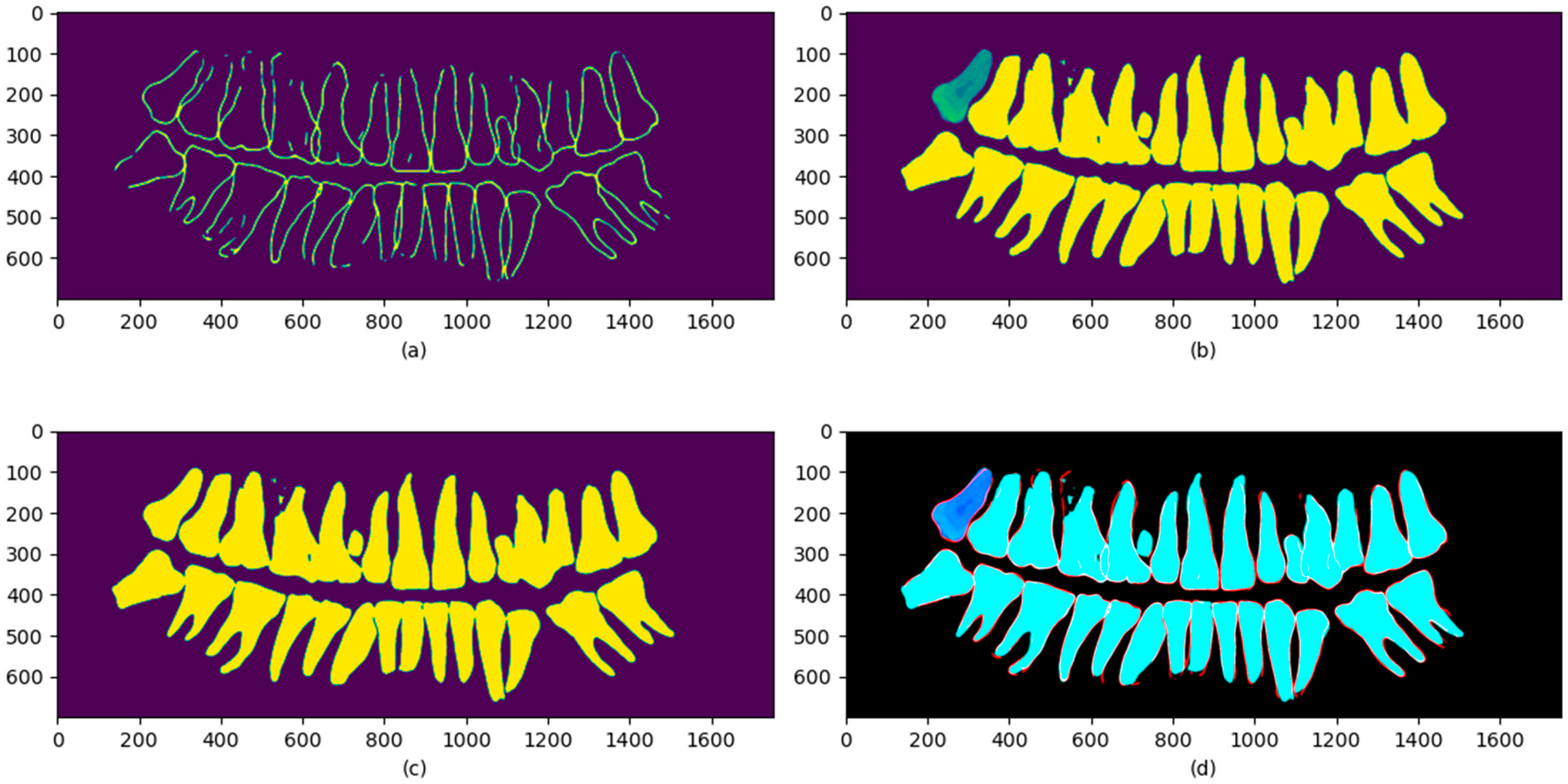
3.3. Single-Object Segmentation Image Generation Method Based on Information Entropy Compression Using Few-Shot Datasets

The generation of the object center allows the model to find the approximate position of each object, and then, to obtain the object instance of each object through a method based on deep learning. Given that medical images are often considerably noisy, it is difficult to obtain the central point image of an object through inputting the original image. As shown in Equation (2), for a single grayscale image in which each pixel can take a value of 256, the information entropy is relatively large. Additionally, it is difficult for the model to effectively extract more abstract image features under few-shot, but the information entropy of the image can be considerably reduced without losing the need to determine the central point of the object key information. As shown in Equation (3), in a multi-channel binarized image, the information entropy of a two-dimensional image is the sum of the information entropy of each channel image. In comparison with the information entropy of the gray image, the original 256-level gray image becomes a binarized multi-channel image, resulting in a significant reduction in the information entropy of the new image, compared with the original grayscale image. Therefore, extracting semantic features and edge images with less interference through U-Net before extracting the object center can effectively reduce the information entropy of the image. As shown in Figure 1, the original image in the figure was obtained using two deep learning models, i.e., semantic segmentation and edge images. Evidently, we can still assess the position of the object central point from the synthetic image of semantics and edges. In Equation (2), $H_0$ shows the information entropy of a grayscale image, $P_i$ is the probability of a certain gray level in the image, which can be obtained from the gray level histogram; in Equation (3), $H_{binary}$ is the information entropy of binary multiscale image, $P_{i,j}$ is the probability of a certain level in the image channel j.

$$H_{0 }=-{{\displaystyle \sum }}_{i=0}^{255}{P}_{i}log{P}_i,$$

(2)

$$H_{binary}=-{\displaystyle \sum }_{i=0}^2{\displaystyle \sum }_{j=0}^1{P}_{i,j}log{P}_{i,j}$$

(3)

For example, for a tooth image (with dimensions 2440 × 1280 pixels), the information entropy $H_0$ of the original grayscale image was 6.861. After it becomes a three-channel binarized structure-related information image, the new image information entropy $H_{binary}$ becomes 1.202, which is about $1/5$ of the original one. At the same time, we found that the shape of each tooth obtained could still be manually distinguished. Therefore, this method can effectively reduce the image information entropy, so that the model can fit the center of the object in the case of a small sample. As shown in Figure 1, the new image only retains the necessary information to determine the center of the object, eliminates unnecessary noise, and makes the input image clearer, compared with the original image. Next, the new image obtained with the deep learning model is used to extract the center of the object, in order to acquire the central point image. Given that the weight of the central point signal output from the trained U-Net model is relatively weak, we modified the central point binarization threshold of the U-Net output from the general 0.3–0.7 range to 0.1, and the binarization formula is as follows:

$$y_{i, j}=1 if y_{i, j}>0.1, else y_{i, j}=0,$$

(4)

In Equation (4), $y_{i,j}$ represents the pixel value of row i and column j in the U-Net output picture. Figure 1 indicates that the U-Net obtains semantic segmentation and edge images from the original image; we input the semantic segmentation and edge images after channel splicing into the U-Net model for central point extraction, and the output image is the central point image of the objects.

After obtaining the object central point image, each center needs to be processed for connected region separation, to separate each object. For example, 30 central points were obtained for a certain result. After passing through the connected region algorithm, 30 single-center images were obtained. The connected region algorithm used in this study is the seeded region growing algorithm. The detailed process is presented in Algorithm 2. In Algorithm 2, each pixel needs to be accessed; in the most extreme case, each pixel will be marked as a connected area. In this article, 4 connections are used to determine whether they are connected, so the time complexity is O (4 ∗ mn) = O (mn), m and n indicates the length and width of the image.

Algorithm 2

INPUT: Edge segmentation image S OUTPUT: Output Image So Parameters: Fill Color Cf,      Boundary Color Cb Function Seedfilling (x, y, S, Cf, Cb):   $c:=S_{x, y}$ If c not equals tIf c not equals to Cf and c not equals to Cb:   $S_{x,y}=C_f$   Seedfilling (x + 1, y, Cf, Cb)   Seedfilling (x − 1, y, Cf, Cb)   Seedfilling (x, y + 1, Cf, Cb)   Seedfilling (x, y − 1, Cf, Cb)

After obtaining the central point image of each object, we sequentially superimpose the centers of the single object, semantic, and edge images to obtain new samples, and use U-Net to obtain the semantic segmentation image of a single object. As shown in Figure 6, the network model regresses the semantic segmentation image of a single object based on semantic and edge models. The acquired input and single-object images are shown in Figure 6, where the input image was generated from the test image.

Figure 6. Single-object segmentation image extraction.

3.4. Teeth Classification Method Based on Fusion of Semantic Images

After extracting the object, the next task is to determine the category of each object. For example, if an incisor is encountered, the output is the incisor category; otherwise, if a third molar is encountered, the output is the category of the third molar, and so on. Generally, in the case of small-sample training without transfer learning, the ability of traditional deep neural networks to evaluate teeth categories may be reduced. The reasons for the decrease in accuracy are not only because of the small sample size, but also the images between teeth categories. As shown in Figure 7, the training pictures of different types of teeth are not highly distinguishable.

Figure 7. Different teeth images. (a,b) are from same person, and (a) is the Lateral incisor, (b) is the Central incisor.

When dentists assess the type of teeth, they will rely on the shape structure and relative position structure of the teeth. On this basis, this method adds the relative position needed to judge the object type of the teeth with the original classification network information, so that the network has a certain improvement in the classification ability of few-shot of teeth.

The addition of relative position information can add the positional information of the teeth to the input image; however, this mechanism will cause the network to rely too much on the position itself for the assessment of the object category, and ignore the shape information of the teeth. To solve this problem, this method embeds the grayscale image of a single dental object into the semantic image (shown in Figure 8b), and combines the embedded grayscale, the semantic segmentation, and the object edge images through the channel stitching method, to synthesize a new multiple-channel image named the “teeth structure semantic information fusion map”. The new image not only retains the image features of the dental object, but also provides relative position information for the model; thus, the classification ability of the model is remarkably improved compared to the original image classification. A generated tooth structure semantic information fusion image is shown in Figure 8.

Figure 8. Teeth classification using structural semantic information. (a) The tooth edge image, (b) The tooth grayscale image embedded in a semantic segmentation image, (c) The semantic segmentation teeth image, and (d) The image spliced by (a–c).

In Figure 8, Figure 8a is the tooth edge image, Figure 8b is the tooth grayscale image embedded in a semantic segmentation image, Figure 8c is the semantic segmentation teeth image, and Figure 8d is the image spliced by Figure 8a–c; Figure 8a is in the red channel of the RGB image, Figure 8b is in the green channel, and Figure 8c is in the blue channel. The algorithm for image generation is presented in Algorithm 3. Each pixel needs to be accessed in Algorithm 3, so the time complexity is O (mn), and m and n represent the length and width of the image.

Algorithm 3

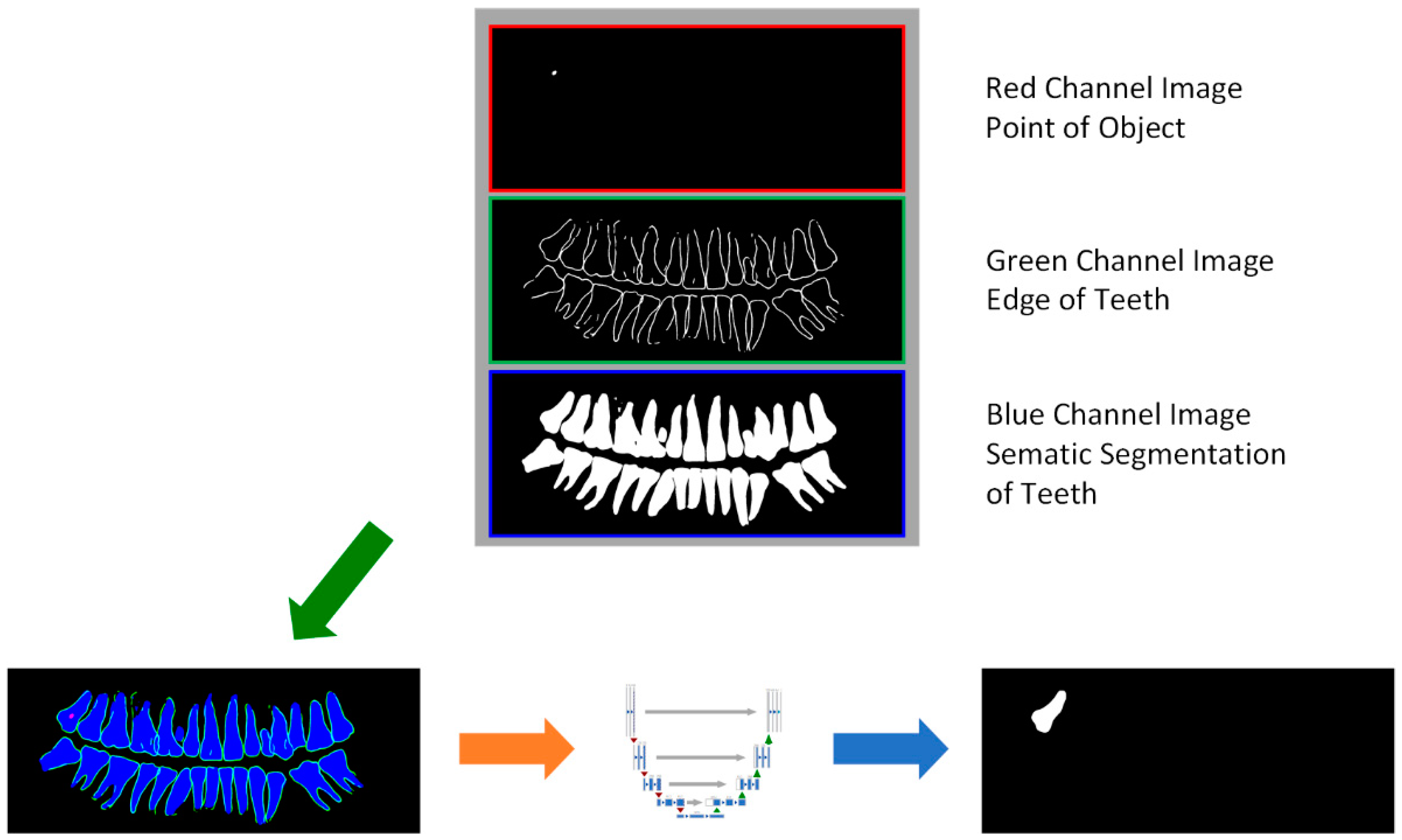
INPUT: Edge segmentation image S1      Semantic segmentation image S2      Single tooth segmentation image S3 OUTPUT: Output Image S0 S0 is a new RGB image length and width is same as S1 For i in (0, length of S1): For j in (0, width of S1):    If S3i,j equals to 0:      S0i,j,G = S2i,j    Else:      S0i,j,G = S3i,j    Endif S0R = S1 S0B = S2

In terms of classification methods, this paper used Resnet as a classification model, which is a reliable model structure, and the overall structure is shown in the Figure 9. The residual structure of Resnet can make the expression ability of the network more powerful, and the reason for choosing this model is because Resnet is a high-performance and easy to train structure, it performs well with Cifar10. As this article will classify teeth into eight types, which is similar to 10 classifications, Resnet is used.

Figure 9. VGG, plain network structure, and Resnet network structure comparison diagram; the upper is VGG, the middle is the plain network structure, and the lower is the Resnet network structure.

4. Experiments and Discussion

The process of object detection is generally divided into two tasks: 1. Find the object. 2. Classify the extracted objects. The experiments in this section were set up in three parts, according to the structure of SPSC-NET, and as shown in Figure 1: 4.2 the extraction of key points of teeth test, 4.3 tooth classification ability test, and 4.4 tooth object detection ability test. In the key point detection, because this method improved on U-Net and U-Net performs well in small-sample scenarios, the comparison model is U-Net. In the classification test, this paper set up a control group of different models: 1. the advanced classification model efficientnetv2; 2. using the same model (Resnet18) without image data processing; 3. using a pretrain-finetuning method on the same model (Resnet18). In addition, we proved the advantages of low information entropy images in the classification task by setting up ablation experiments. In the object detection ability test experiment, this paper compared with the Faster-RCNN structure commonly used in the dental medical field, and in order to prove the poor performance of the single-stage object detection method in the dental object detection field, a control group was also set up. In addition, an ablation experiment was constructed to demonstrate the improvement of the overall detection ability of the tooth semantic structure information.

4.1. Experimental Setup and Datasets

The dataset of our study contained 110 panoramic dental images. The images were divided into a training dataset composed of 10 images and a test dataset composed of 100 images. This division method was to prove the performance of this method on small-sized datasets, and to prove the reliability of this method with a sufficient validation set; these 110 images were labeled. The labeling tool VGG Image Annotator (VIA), which marks the specific types of teeth while marking the mask of each dental object, was used in this study. We used Palmer’s teeth position notation to divide the teeth into eight categories, namely the central incisors, lateral incisors, and canines. The first premolars, second premolars, first molars, second molars, and third molars were marked with numbers from 1 to 8. The simulations were performed using Linux (Ubuntu20.04LTS), GEFORCE RTX 2080Ti, and Pytorch1.8. Among them, except for the small number of third molar samples corresponding to category 8, the number of samples in the test dataset of the other categories was greater than 300. Table 1 presents the distribution of different types of teeth in the test dataset.

Table 1. Distribution of different types of teeth in test dataset.

Category	Quantity
Central incisor	403
Lateral incisor	399
Canine	397
First premolar	389
Second premolar	400
First molar	395
Second molar	395
Third molar	284

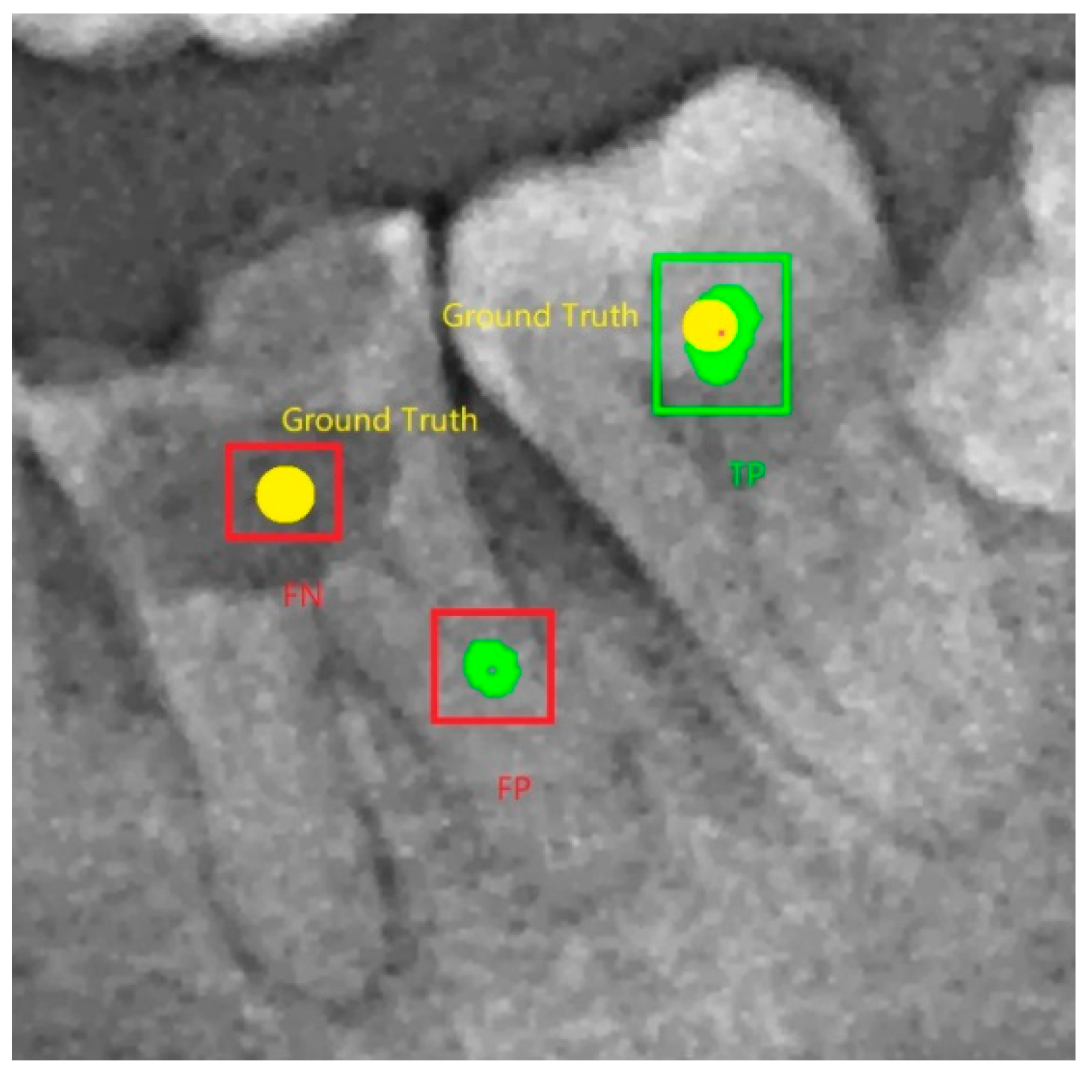
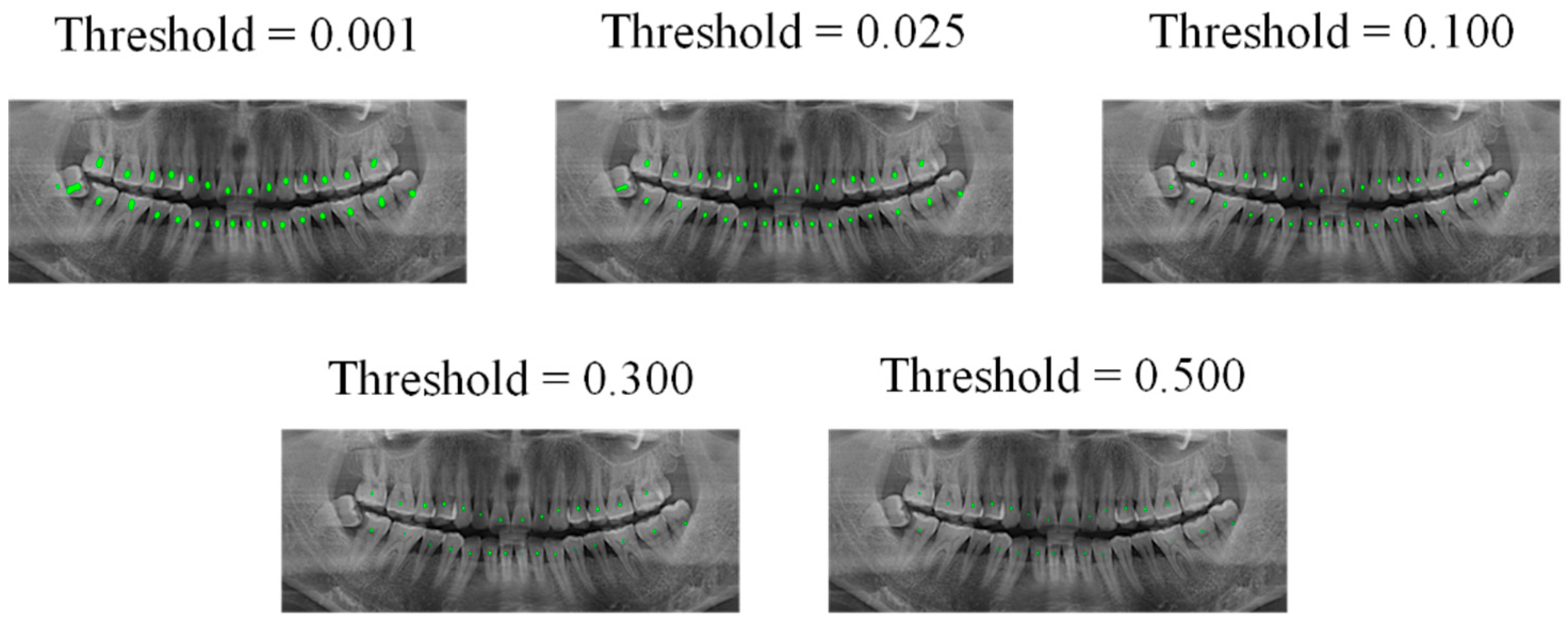
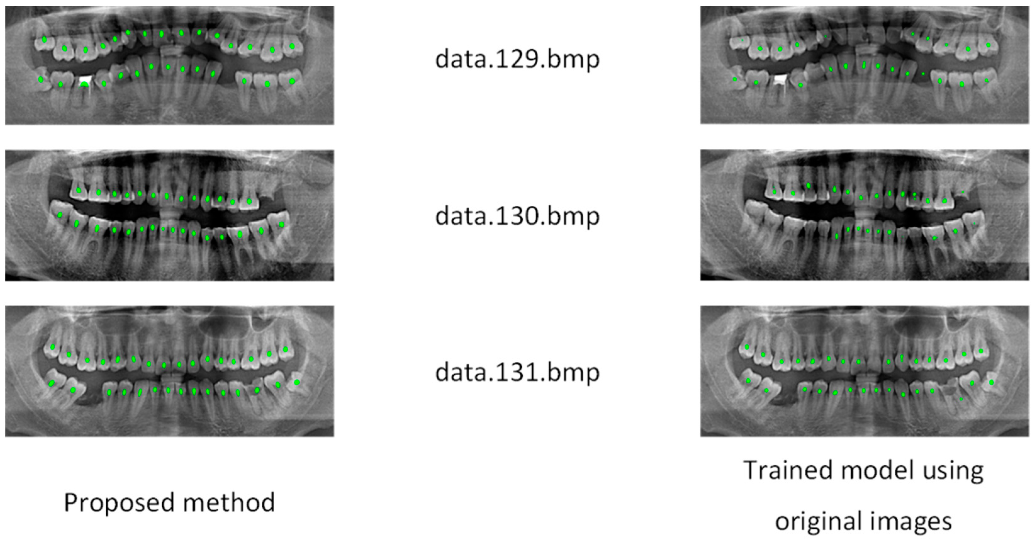
4.2. Teeth Central Point Detection Capability Test

After marking the boundary shape and category, the SPSC-NET method performs data augmentation on the edge and semantic images. In addition to transforming the input image data, the label or mask must be transformed accordingly. In this experiment, the “Augmentor” library was used to enhance the original 10 images into 20,000 images of semantic segmentation and edge images, which were recorded as datasets A and B.

Subsequently, two deep learning models were trained using datasets A and B; both models were U-Net, and due to our hardware limitations, we set the batch-size to 1, the learning rate to 0.01, and the epochs to 9. Then, we input the 10 processed images into the model trained in dataset B to obtain 20 edge images with threshold values of 0.5 and 0.94, and used the channel stitching method to stitch these edge images with the semantic segmentation mask, to obtain 20 processed images. In the next step, the VIA tool was used to mark the central points of these 20 images, perform image augmentation, and mark it as dataset C. Dataset C was used for training the new U-Net model. The effects of the measured model at output thresholds of 0.001, 0.025, 0.1, 0.3, and 0.5, are shown in Figure 10.

Figure 10. Output of teeth central point dataset under different thresholds.

Figure 10 indicates that if the image output is according to the default output threshold (0.5) of conventional semantic segmentation, the central point image cannot effectively express all object centers of the teeth. However, if the output threshold is set to very low levels, we often encountered adhesion of the object centers of the teeth; based on experience, we set the threshold of the central point output to 0.025, so that all centers can be expressed as much as possible, and they are also well separated.

In this part, the model has two evaluation indicators for the ability to detect the central point of the target: recall and precision, and the formulas for both are as follows:

$$Precision=\frac{TP}{TP+FP}$$

(5)

$$Recall=\frac{TP}{TP+FN}$$

(6)

As shown in Figure 11, this chapter compares the predicted area extracted using SPSC-NET and U-Net with the real target center point (GT value, Ground Truth) in the test set, where:

TP: The center point of the predicted area falls into the GT area.

FP: The center point of the predicted area does not fall into the GT area.

FN: There is no corresponding center point to match the GT area. Note that if the target is not detected or the target point deviates from the center of the target, the FN will be generated.

Figure 11. Criteria for judging the ability to detect the central point. The green area is the predicted area, the magenta dotted object is the central coordinate of the predicted area, the yellow area is the GT area, the green box is TP, and the red box is FN and FP.

From the definitions of TP, FN, and FP, it can be seen that the value range between the precision and recall value evaluation index is 0–100%.

The effect of the improved U-Net was compared with that of the original U-Net model, as shown in Figure 12. In the case of the same three images (the model output threshold is also the same), the dental object center generated based on the fusion image was obviously better than the original image training method. The SPSC-NET method was also superior in terms of specific data. The values in Table 2 of the paper show that SPSC-NET was between 99–100% for both the recall and precision indicators. In the precision test, the SPSC-NET was slightly ahead of the original U-Net in the case of a low output threshold; and in the recall rate test, it was approximately 2.87%, although it was at a low level. In the case of the threshold value, the SPSC-NET was slightly better, but the output image effect under a low threshold value was not good; hence, there was often a problem of adhesion of the object center. In the case of a high threshold value, the SPSC-NET was obviously ahead of the original U-Net for the recall value. The recall value reflects the hits in the positive sample in this experiment; therefore, the SPSC-NET had a significantly lower rate of missed detection of the object central point.

Figure 12. Image comparison between the generated teeth central point based on the structural semantic information and the original segmentation network.

Table 2. Comparison of generated teeth central point based on the structural semantic information and the original segmentation network.

Out Threshold	Precision		Recall
	SPSC-NET	Native U-Net	SPSC-NET	Native U-Net
0.001	99.77	99.36	99.54	96.67
0.025	99.80	99.50	99.23	94.76
0.100	99.82	99.60	98.85	92.39
0.300	99.84	99.66	98.03	88.99
0.500	99.86	99.70	96.16	85.39

SPSC-NET is better at extracting the target center point in a small-size dataset because it uses information about the semantic structure of the tooth as a priori knowledge. This a priori knowledge can exclude interfering information before extracting the center points of the targets, although the performance of U-Net in a small-size dataset is acceptable, but adding more prior knowledge gives better performance. The original U-Net network structure is not good enough without the help of a priori knowledge, so in SPSC-NET was designed a structure for extracting the a priori knowledge information, to determine the tooth’s target center point more efficiently.

After obtaining the center of the dental object, the next step is to obtain the segmented image of a single object. The marked central point image was separated into separate central points, and these were combined with those obtained by U-Net segmentation. The semantics and edge images were combined with the channel, and the mask of each image corresponds to the segmented image of a single tooth, where the central point of each image is located. Similarly, these images were augmented and marked as “Dataset D”, which was used as the training dataset of the single-object segmentation image model for training. The model was U-Net, and there were nine epochs. In the test results, the Dice coefficient value of the single-object segmentation image model was 0.9701, and its calculation formula is defined as:

$$\mathrm{Dice} \mathrm{coefficient}=\frac{2\left|X{\displaystyle \cap }Y\right|}{\left|X\right|+\left|Y\right|}$$

(7)

4.3. Teeth Classification Capability Test

As mentioned in 3.3, high image information entropy will interfere with the DNN model, making the model learn many non-robust features. In 3.4, this paper implements a multi-channel tooth semantic structure information map, because in the image, most of the pixel values are binarized, so the information entropy of the image is low. In order to prove the advantages of the low information entropy image, this paper designs a tooth semantic structure map with high information entropy as the ablation experimental sample. The high information entropy also provides the DNN classification model with the global information of the teeth, the position information of the teeth and the shape information of the teeth. The specific construction method is relatively simple. The segmented image of the object instance of the tooth is inserted into the blue channel of the original tooth grayscale image, as shown in Figure 13. Theoretically, the image contains all the features in the tooth semantic structure information map proposed in 3.4, but the information entropy is higher than in the tooth semantic structure information map.

Figure 13. In order to prove the effectiveness of the information entropy compression method, a high information entropy tooth semantic structure information map was constructed, which still includes the position and shape features of the teeth, and also includes the global tooth features.

4.3.1. Datasets

In order to test the accuracy of the classification model, three datasets were produced in the experiment: 1. Use the method in 3.4 to generate a tooth semantic structure information map. 2. Use the high information entropy tooth semantic structure information map just mentioned, and use image enhancement, including image rotation, image mirror rotation, elastic deformation, and random scaling. 3. Cut out each tooth individually to make a square image. The effect is shown in Figure 7. The significance of setting this control group is that this experiment simulates a classification scene without using the tooth semantic structure information. At the same time, in order to prove the effect of image enhancement on the improvement of the model, this paper conducted data enhancement comparison experiments on dataset 1 and dataset 3. The method of image enhancement was the same as that of dataset 2.

4.3.2. Models

In order to demonstrate the improvement of the classification ability of the semantic structure information map, Resnet18 was used to classify the tooth semantic structure information map. The efficientnetv2, Resnet18, and Resnet18 networks based on ImageNet pre-training (ft stands for pre-training fine-tuning) were used to classify dataset 3. In terms of hyperparameter settings, the initial learning rate of these models was 0.01, and then every 200 epochs were multiplied by 0.1; the number of epochs was 800, and the batch-size was 20. The results of the test set were as in Figure 14.

Figure 14. Comparison of the accuracy and loss curves of different methods under the same model. Different marker shapes represent different dataset types. The dots represent the classification of tooth semantic structure information images. The inverted triangle represents the tooth semantic structure information map with high information entropy, the asterisks represent common single-tooth classification images. The solid line represents the image processed by the image enhancement method, and the dashed line represents the image without using the image enhancement method.

As shown in Table 3, in this experiment, the accuracy rate of the training task constructed with fused tooth semantic structure information images was 96.05, which is 33.67% higher than the original Resnet classification method. In comparison using the same image enhancement method, the SPSC-NET method still maintained a relatively large lead, which was 21.85%. Compared with the more advanced efficientnetv2, the lead was still relatively large; and it is worth noting that after the image enhancement, the accuracy of the classification method using the tooth semantic structure information map had been improved somewhat, and the loss of the model at the end of the training was the same, and the accuracy was basically close to convergence. In comparison with the classification method of the tooth semantic structure information image with high information entropy, the image classification result of low information entropy was about 3.5% lower than the classification result of high information entropy. The classification method of tooth semantic structure information compressed with information entropy was effective.

Table 3. Comparison results of different methods under the same model.

Models	Accuracy	Precision	F1score	Loss
Resnet + structural information (ours)	96.05	96.10	96.05	0.00644
Resnet + structural information- 1 (ours)	92.49	92.56	92.49	0.01286
Efficientnetv2-m	74.76	75.58	74.90	0.11094
Resnet + ft	59.90	60.20	59.70	0.15345
Resnet	74.20	74.98	74.31	0.04754
Resnet + structural information (ours) (Without data augmentation)	94.12	94.20	94.13	0.00902
Efficientnetv2-m (Without data augmentation)	63.72	64.06	63.55	0.10600
Resnet + ft (Without data augmentation)	51.53	51.22	51.06	0.31689
Resnet (Without data augmentation)	62.38	63.11	62.44	0.12297

¹ Structural information- is high information entropy tooth semantic structure information map for comparison.

4.4. Teeth Detection Capability Test

This round of experiments compared the SPSC-NET method with Faster-RCNN, Retina-net, SSD, and SSD-lite methods; it should be noted that our purpose in testing Faster-RCNN was to reproduce the work of Laishram et al. [16]. At the same time, in order to compare the performance of Faster-RCNN in the original text, we also compared the raw data of Faster-RCNN in the text (the training images was 96, but there was no AP₅₀, AP₇₅ and mIOU in that paper). In addition, to demonstrate the effectiveness of few-shot object detection learning on dental detection tasks, we also reproduced the performance of TFA, including TFA based on full connection and TFA based on cosine similarity. Faster-RCNN, Retina-net, SSD, SSD-lite, and TFA model training adopted the transfer learning method, pre-training on the basis of COCO2017 data set pre-training, and then fine-tuning training on the small-sample tooth object detection training set. In terms of settings, the learning rates of Faster-RCNN, Retina-net, SSD, and SSD-lite were all 0.01, and the steps were 200; multiplied by 0.1, epochs were 800, batch-size was set to 20, and the confidence threshold of the output result of Faster-RCNN was set to 0.5. Since the default confidence threshold was low, at 0.05, there were a lot of duplicate and misclassified prediction boxes. In the hyperparameter setting of TFA, iter was set to 20,000, batch-size was set to 20, and the rest used the default parameters of the original author of TFA. In the SSD and SSD-lite models, the corresponding data enhancement methods of SSD were used, including random image photometric distortion, scaling, mIOU-based cropping, and horizon flipping. Other parameters were the torchvision default values, and the AP value [56] was tested after training. Before the AP evaluation, the output format of SPSC-NET needed to be converted. Since the SPSC-NET method outputs some single-object segmentation images instead of bounding boxes, it is necessary to take the four largest coordinate values of the upper, lower, left, and right of the single-segmented image as the object detected box (x1, y1, x2, y2). At the same time, this experiment also designed an ablation experiment comparison; that is, using the object bounding box generation method proposed in this paper and the task of classifying the grayscale image of a single tooth, called SPSC-NET. In the AP test results, the object detection effect of SPSC-NET was much better than that of Faster-RCNN. As shown in Table 4, ft in the table represents fine-tuning, which shows that the object detection ability of SPSC-NET under few-shot was higher, and the ability to cover the object was stronger. The worst performance class in the SPSC-NET method was the 8th class with the smallest sample size. For the precision–recall curve, the precision–recall curve of the 8th class was still sufficient to lead the best performing class of Faster-RCNN, as shown in Figure 15; Figure 15a is the worst category precision–recall curve of this method, and Figure 15b is the best category precision–recall curve when the Faster-RCNN Box score = 0.8.

Table 4. Comparison of results between SPSC-NET and other methods.

Model	AP	AP50	AP75	mIOU	Train Image
Retinanet + ft	12.76%	15.25%	10.26%	0.2602	10
SSD + ft	1.67%	2.68%	0.63%	0.3077	10
SSD Lite + ft	11.98%	15.57%	8.38%	0.1557	10
Faster-RCNN [16] + ft (Laishram et al., Box score = 0.3)	73.56%	86.42%	60.69%	0.6063	10
Faster-RCNN [16] + ft (Laishram et al., Box score = 0.5)	72.26%	84.61%	59.91%	0.6334	10
Faster-RCNN [16] (Laishram et al.)	91.03%	N/A	N/A	N/A	96
Chung et al. [46] (33 classes)	81%	91%	90%	0.84	818
TFA w/fc [42]	21.82%	49.13%	15.14%	N/A	10
TFA w/cos [42]	32.06%	48.43%	15.69%	N/A	10
SPSC-NET	88.28%	92.94%	83.62%	0.8031	10
SPSC-NET-	19.41%	20.39%	18.43%	0.5028	10

Figure 15. Comparison of precision–recall curves of the category with the lowest AP of the proposed method (a) and category with the highest AP of the Faster R-CNN (b).

As shown in Table 4, the object detection ability of SPSC-NET in the case of few-shot was significantly improved compared to Faster-RCNN. The reason for this phenomenon is that SPSC-NET uses images of tooth semantic structure information. The object detection ability of the model in the training process was significantly enhanced, and the SPSC-NET was more powerful in the object classification, due to the use of the tooth object classification method based on the fusion semantic image. Based on the above reasons, the object detection ability of SPSC-NET was better than that of Faster-RCNN. At the same time, we also found that, although the AP value of Faster-RCNN is better when the box score is very low, the performance of its mIOU is even worse. The actual performance of the two is shown in Figure 16: Figure 16a is the output of the SPSC-NET method, and Figure 16b is the output of the Faster-RCNN when the box score is 0.3. Red is the wrong ROI, and green is the correct ROI. From the detection in the figure, although the AP value of Faster-RCNN-based tooth object detection reached 73.56, due to the defects of the AP value, as the number of frames increased, the performance decline did not affect the AP value when the recall value unchanged, and the decrease in the accuracy rate did not affect the AP score, so the actual performance of Faster-RCNN was much worse than the performance on the AP data indicator. According to the results of the work of Laishram et al. [16], the Faster-RCNN performance was higher after training with 96 images. This proves that with the same model, the increase in the training image improves the model performance of Faster-RCNN. It is also worth noting that in our comparison, the single-stage object detector based on transfer learning was not of practical value for the performance, which is consistent with the review results of Singh et al. [25]. In addition, the TFA method in the field of small-sample object detection did not perform well in our tests, which can confirm why there is little research in the field of dental detection using the FSOD method; the reason for this phenomenon is because TFA relies on the base dataset, and using the generic dataset as the base dataset will cause the source domain to mismatch the target domain. Unlike Faster-RCNN, if the researchers want to apply the FSOD method to the field of tooth target detection, they need to conduct more in-depth research on the FSOD models and the feature of tooth detection data.

Figure 16. Image comparison between (a) SPSC-NET and (b) Faster R-CNN when box score is 0.3.

5. Conclusions

This paper proposes a U-Net-based object detection method, SPSC-NET, which performs well on small-scale dental image datasets. Our contributions are mainly as follows:

• The center point detection method based on the fusion of tooth structure semantics can generate center points of objects under a small-size dataset; and from the perspective of symmetry, the network for extracting the tooth structure semantics information is a symmetric structure, compared with the direct use of the semantic segmentation model, and the precision and recall rate of the SPSC-NET method reached 99.84 and 99.29.
• The performance of the proposed image generation mechanism for tooth semantic structure information in the classification of few-shot was much ahead of that based on the original image classification method (using DNN models directly), and its information entropy compression method can effectively improve the classification performance of the model.
• In terms of AP indicators and precision–recall curve, the object detection effect of SPSC-NET was better than that of Faster-RCNN, and it is more advantageous in the case of few-shot. The proposed tooth semantic structure information map can help the model greatly improve its final object detection performance. In the field of medical image research, image segmentation is a hot topic. The object detection method based on U-Net proposed in this paper can provide more ideas for subsequent medical image research. In addition, since SPSC-NET outputs single-object segmentation images and categories, in theory, this method can generate instance segmentation images.

References

1. Rampersad, H. Faster R-CNN: Towards Real-Time Object Detection with Region Proposal Networks. Adv. Neural Inf. Process. Syst. 2020, 28, 159–183. [Google Scholar] [CrossRef]
2. Ronneberger, O.; Fischer, P.; Brox, T. U-Net: Convolutional networks for biomedical image segmentation. In Medical Image Computing and Computer-Assisted Intervention 2015; Lecture Notes in Computer Science (Including Subseries Lecture Notes in Artificial Intelligence and Lecture Notes in Bioinformatics); Springer: Cham, Switzerland, 2015; Volume 9351, pp. 234–241. [Google Scholar] [CrossRef] [Green Version]
3. Shelhamer, E.; Long, J.; Darrell, T. Fully convolutional networks for semantic segmentation. IEEE Trans. Pattern Anal. Mach. Intell. 2017, 39, 640–651. [Google Scholar] [CrossRef]
4. Li, C.; Tan, Y.; Chen, W.; Luo, X.; He, Y.; Gao, Y.; Li, F. ANU-Net: Attention-based nested U-Net to exploit full resolution features for medical image segmentation. Comput. Graph. 2020, 90, 11–20. [Google Scholar] [CrossRef]
5. Sambyal, N.; Saini, P.; Syal, R.; Gupta, V. Modified U-Net architecture for semantic segmentation of diabetic retinopathy images. Biocybern. Biomed. Eng. 2020, 40, 1094–1109. [Google Scholar] [CrossRef]
6. Diakogiannis, F.I.; Waldner, F.; Caccetta, P.; Wu, C. ResUNet-a: A deep learning framework for semantic segmentation of remotely sensed data. ISPRS J. Photogramm. Remote Sens. 2020, 162, 94–114. [Google Scholar] [CrossRef] [Green Version]
7. Li, X.; Chen, H.; Qi, X.; Dou, Q.; Fu, C.-W.; Heng, P.-A. H-DenseUNet: Hybrid Densely Connected UNet for Liver and Tumor Segmentation From CT Volumes. IEEE Trans. Med. Imaging 2018, 37, 2663–2674. [Google Scholar] [CrossRef] [Green Version]
8. Wang, C.-W.; Huang, C.-T.; Lee, J.-H.; Li, C.-H.; Chang, S.-W.; Siao, M.-J.; Lai, T.-M.; Ibragimov, B.; Vrtovec, T.; Ronneberger, O.; et al. A benchmark for comparison of dental radiography analysis algorithms. Med. Image Anal. 2016, 31, 63–76. [Google Scholar] [CrossRef]
9. Duong, D.Q.; Nguyen, K.C.T.; Kaipatur, N.R.; Lou, E.H.; Noga, M.; Major, P.W.; Punithakumar, K.; Le, L.H. Fully Automated Segmentation of Alveolar Bone Using Deep Convolutional Neural Networks from Intraoral Ultrasound Images. In Proceedings of the Annual International Conference of the IEEE Engineering in Medicine and Biology Society, EMBS, Berlin, Germany, 23–27 July 2019; pp. 6632–6635. [Google Scholar] [CrossRef]
10. Koch, T.L.; Perslev, M.; Igel, C.; Brandt, S.S. Accurate segmentation of dental panoramic radiographs with U-NETS. In Proceedings of the 2019 IEEE 16th International Symposium on Biomedical Imaging (ISBI 2019), Venice, Italy, 8–11 April 2019; pp. 15–19. [Google Scholar] [CrossRef]
11. Gherardini, M.; Mazomenos, E.; Menciassi, A.; Stoyanov, D. Catheter segmentation in X-ray fluoroscopy using synthetic data and transfer learning with light U-nets. Comput. Methods Programs Biomed. 2020, 192, 105420. [Google Scholar] [CrossRef]
12. Chen, Y.; Du, H.; Yun, Z.; Yang, S.; Dai, Z.; Zhong, L.; Feng, Q.; Yang, W. Automatic Segmentation of Individual Tooth in Dental CBCT Images From Tooth Surface Map by a Multi-Task FCN. IEEE Access 2020, 8, 97296–97309. [Google Scholar] [CrossRef]
13. Xu, X.; Liu, C.; Zheng, Y. 3D Tooth Segmentation and Labeling Using Deep Convolutional Neural Networks. IEEE Trans. Vis. Comput. Graph. 2019, 25, 2336–2348. [Google Scholar] [CrossRef]
14. Zhao, Y.; Li, P.; Gao, C.; Liu, Y.; Chen, Q.; Yang, F.; Meng, D. TSASNet: Tooth segmentation on dental panoramic X-ray images by Two-Stage Attention Segmentation Network. Knowl.-Based Syst. 2020, 206, 106338. [Google Scholar] [CrossRef]
15. Al Kheraif, A.A.; Wahba, A.A.; Fouad, H. Detection of dental diseases from radiographic 2d dental image using hybrid graph-cut technique and convolutional neural network. Measurement 2019, 146, 333–342. [Google Scholar] [CrossRef]
16. Laishram, A.; Thongam, K. Detection and classification of dental pathologies using faster-RCNN in orthopantomogram radiography image. In Proceedings of the 2020 7th International Conference on Signal Processing and Integrated Networks, SPIN 2020, Noida, India, 27–28 February 2020; pp. 423–428. [Google Scholar] [CrossRef]
17. Tuzoff, D.V.; Tuzova, L.N.; Bornstein, M.M.; Krasnov, A.S.; Kharchenko, M.A.; Nikolenko, S.I.; Sveshnikov, M.M.; Bednenko, G.B. Tooth detection and numbering in panoramic radiographs using convolutional neural networks. Dentomaxillofac. Radiol. 2019, 48, 20180051. [Google Scholar] [CrossRef]
18. Chen, H.; Zhang, K.; Lyu, P.; Li, H.; Zhang, L.; Wu, J.; Lee, C.-H. A deep learning approach to automatic teeth detection and numbering based on object detection in dental periapical films. Sci. Rep. 2019, 9, 3840. [Google Scholar] [CrossRef] [Green Version]
19. He, K.; Gkioxari, G.; Dollár, P.; Girshick, R. Mask R-CNN. IEEE Trans. Pattern Anal. Mach. Intell. 2020, 42, 386–397. [Google Scholar] [CrossRef]
20. Cui, Z.; Li, C.; Wang, W. ToothNet: Automatic tooth instance segmentation and identification from cone beam CT images. In Proceedings of the IEEE Conference on Computer Vision and Pattern Recognition, Long Beach, CA, USA, 16–20 June 2019; pp. 6368–6377. [Google Scholar]
21. Moutselos, K.; Berdouses, E.; Oulis, C.; Maglogiannis, I. Recognizing Occlusal Caries in Dental Intraoral Images Using Deep Learning. In Proceedings of the Annual International Conference of the IEEE Engineering in Medicine and Biology Society, EMBS, Berlin, Germany, 23–27 July 2019; pp. 1617–1620. [Google Scholar] [CrossRef]
22. Jader, G.; Fontineli, J.; Ruiz, M.; Abdalla, K.; Pithon, M.; Oliveira, L. Deep Instance Segmentation of Teeth in Panoramic X-Ray Images. In Proceedings of the 31st Conference on Graphics, Patterns and Images, SIBGRAPI 2018, Parana, Brazil, 17 January 2019; pp. 400–407. [Google Scholar] [CrossRef]
23. Bochkovskiy, A.; Wang, C.Y.; Liao, H.Y.M. YOLOv4: Optimal Speed and Accuracy of Object Detection. arXiv 2020. [Google Scholar] [CrossRef]
24. Liu, W.; Anguelov, D.; Erhan, D.; Szegedy, C.; Reed, S.; Fu, C.Y.; Berg, A.C. SSD: Single shot multibox detector. In Proceedings of the European Conference on Computer Vision, Amsterdam, The Netherlands, 11–14 October 2016; Volume 9905, pp. 21–37. [Google Scholar] [CrossRef] [Green Version]
25. Singh, N.K.; Raza, K. Progress in deep learning-based dental and maxillofacial image analysis: A systematic review. Expert Syst. Appl. 2022, 199, 116968. [Google Scholar] [CrossRef]
26. Krizhevsky, A.; Sutskever, I.; Hinton, G.E. ImageNet Classification with Deep Convolutional Neural Networks. Adv. Neural Inf. Process. Syst. 2012, 25. Available online: https://proceedings.neurips.cc/paper/2012/hash/c399862d3b9d6b76c8436e924a68c45b-Abstract.html (accessed on 9 April 2022). [CrossRef]
27. Simonyan, K.; Zisserman, A. Very deep convolutional networks for large-scale image recognition. In Proceedings of the 3rd International Conference on Learning Representations, ICLR 2015-Conference Track Proceedings, San Diego, CA, USA, 7–9 May 2015; pp. 1–14. [Google Scholar] [CrossRef]
28. Hiraiwa, T.; Ariji, Y.; Fukuda, M.; Kise, Y.; Nakata, K.; Katsumata, A.; Fujita, H.; Ariji, E. A deep-learning artificial intelligence system for assessment of root morphology of the mandibular first molar on panoramic radiography. Dentomaxillofac. Radiol. 2019, 48, 20180218. [Google Scholar] [CrossRef]
29. Lee, J.-H.; Kim, D.-H.; Jeong, S.-N.; Choi, S.-H. Diagnosis and prediction of periodontally compromised teeth using a deep learning-based convolutional neural network algorithm. J. Periodontal Implant Sci. 2018, 48, 114–123. [Google Scholar] [CrossRef] [Green Version]
30. Miki, Y.; Muramatsu, C.; Hayashi, T.; Zhou, X.; Hara, T.; Katsumata, A.; Fujita, H. Classification of teeth in cone-beam CT using deep convolutional neural network. Comput. Biol. Med. 2017, 80, 24–29. [Google Scholar] [CrossRef] [PubMed]
31. Muramatsu, C.; Morishita, T.; Takahashi, R.; Hayashi, T.; Nishiyama, W.; Ariji, Y.; Zhou, X.; Hara, T.; Katsumata, A.; Ariji, E.; et al. Tooth detection and classification on panoramic radiographs for automatic dental chart filing: Improved classification by multi-sized input data. Oral Radiol. 2021, 37, 13–19. [Google Scholar] [CrossRef] [PubMed]
32. Yang, J.; Xie, Y.; Liu, L.; Xia, B.; Cao, Z.; Guo, C. Automated Dental Image Analysis by Deep Learning on Small Dataset. In Proceedings of the 2018 IEEE 42nd Annual Computer Software and Applications Conference (COMPSAC), Tokyo, Japan, 23–27 June 2018; Volume 1, pp. 492–497. [Google Scholar] [CrossRef]
33. Zhang, K.; Wu, J.; Chen, H.; Lyu, P. An effective teeth recognition method using label tree with cascade network structure. Comput. Med. Imaging Graph. 2018, 68, 61–70. [Google Scholar] [CrossRef] [PubMed]
34. Oktay, A.B. Tooth detection with Convolutional Neural Networks. In Proceedings of the 2017 Medical Technologies National Congress (TIPTEKNO), Trabzon, Turkey, 12–14 October 2017; pp. 1–4. [Google Scholar] [CrossRef]
35. Son, L.H.; Tuan, T.M.; Fujita, H.; Dey, N.; Ashour, A.; Ngoc, V.T.N.; Anh, L.Q.; Chu, D.-T. Dental diagnosis from X-Ray images: An expert system based on fuzzy computing. Biomed. Signal Process. Control 2018, 39, 64–73. [Google Scholar] [CrossRef]
36. Avuçlu, E.; Başçiftçi, F. The determination of age and gender by implementing new image processing methods and measurements to dental X-ray images. Measurement 2020, 149, 106985. [Google Scholar] [CrossRef]
37. Antonelli, S.; Avola, D.; Cinque, L.; Crisostomi, D.; Foresti, G.L.; Galasso, F.; Marini, M.R.; Mecca, A.; Pannone, D. Few-Shot Object Detection: A Survey. ACM Comput. Surv. 2021. [Google Scholar] [CrossRef]
38. Kang, B.; Liu, Z.; Wang, X.; Yu, F.; Feng, J.; Darrell, T. Few-shot Object Detection via Feature Reweighting. In Proceedings of the IEEE/CVF International Conference on Computer Vision, Seoul, Korea, 27 October–2 November 2019; pp. 8420–8429. [Google Scholar]
39. Yan, X.; Chen, Z.; Xu, A.; Wang, X.; Liang, X.; Lin, L. Meta R-CNN: Towards General Solver for Instance-level Low-shot Learning. In Proceedings of the IEEE/CVF International Conference on Computer Vision, Seoul, Korea, 27 October–2 November 2019; pp. 9577–9586. [Google Scholar]
40. Pérez-Rúa, J.-M.; Zhu, X.; Hospedales, T.; Xiang, T. Incremental few-shot object detection. In Proceedings of the IEEE/CVF Conference on Computer Vision and Pattern Recognition, Seattle, WA, USA, 13–19 June 2020; pp. 13846–13855. Available online: http://openaccess.thecvf.com/content_CVPR_2020/html/Perez-Rua_Incremental_Few-Shot_Object_Detection_CVPR_2020_paper.html (accessed on 16 April 2022).
41. Xiao, Y.; Marlet, R. Few-shot object detection and viewpoint estimation for objects in the wild. In Computer Vision—ECCV 2020; Lecture Notes in Computer Science (Including Subseries Lecture Notes in Artificial Intelligence and Lecture Notes in Bioinformatics); Springer: Cham, Switzerland, 2020; Volume 12362, pp. 192–210. [Google Scholar] [CrossRef]
42. Wang, X.; Huang, T.E.; Darrell, T.; Gonzalez, J.E.; Yu, F. Frustratingly Simple Few-Shot Object Detection. arXiv 2020, arXiv:2003.06957. [Google Scholar] [CrossRef]
43. Fan, Q.; Zhuo, W.; Tang, C.-K.; Tai, Y.-W. Few-Shot Object Detection with Attention-RPN and Multi-Relation Detector. In Proceedings of the IEEE/CVF Conference on Computer Vision and Pattern Recognition, Seattle, WA, USA, 13–19 June 2020; pp. 4013–4022. [Google Scholar] [CrossRef]
44. Chen, T.-I.; Liu, Y.-C.; Su, H.-T.; Chang, Y.-C.; Lin, Y.-H.; Yeh, J.-F.; Chen, W.-C.; Hsu, W. Dual-Awareness Attention for Few-Shot Object Detection. arXiv 2021, arXiv:2102.12152. [Google Scholar] [CrossRef]
45. Akselrod-Ballin, A.; Karlinsky, L.; Hazan, A.; Bakalo, R.; Horesh, A.B.; Shoshan, Y.; Barkan, E. Deep learning for automatic detection of abnormal findings in breast mammography. In Deep Learning in Medical Image Analysis and Multimodal Learning for Clinical Decision Support; Springer: Cham, Switzerland, 2017; pp. 321–329. [Google Scholar] [CrossRef]
46. Chung, M.; Lee, J.; Park, S.; Lee, M.; Lee, C.E.; Lee, J.; Shin, Y.-G. Individual tooth detection and identification from dental panoramic X-ray images via point-wise localization and distance regularization. Artif. Intell. Med. 2021, 111, 101996. [Google Scholar] [CrossRef]
47. Vinayahalingam, S.; Xi, T.; Bergé, S.; Maal, T.; de Jong, G. Automated detection of third molars and mandibular nerve by deep learning. Sci. Rep. 2019, 9, 9007. [Google Scholar] [CrossRef]
48. Chen, H.; Wang, Y.; Wang, G.; Qiao, Y. LSTD: A Low-Shot Transfer Detector for Object Detection. In Proceedings of the AAAI Conference on Artificial Intelligence, New Orleans, LA, USA, 2–7 February 2018; p. 32. Available online: https://ojs.aaai.org/index.php/AAAI/article/view/11716 (accessed on 9 April 2022).
49. Chen, X.; Jiang, M.; Zhao, Q. Leveraging Bottom-Up and Top-Down Attention for Few-Shot Object Detection. arXiv 2020. [Google Scholar] [CrossRef]
50. Sun, B.; Li, B.; Cai, S.; Yuan, Y.; Zhang, C. Fsce: Few-shot object detection via contrastive proposal encoding. In Proceedings of the IEEE/CVF Conference on Computer Vision and Pattern Recognition, Nashville, TN, USA, 20–25 June 2021; pp. 7352–7362. [Google Scholar] [CrossRef]
51. Li, Y.; Zhu, H.; Cheng, Y.; Wang, W.; Teo, C.S.; Xiang, C.; Vadakkepat, P.; Lee, T.H. Few-Shot Object Detection via Classification Refinement and Distractor Retreatment. In Proceedings of the IEEE/CVF Conference on Computer Vision and Pattern Recognition, Nashville, TN, USA, 20–25 June 2021; pp. 15395–15403. [Google Scholar]
52. Zhu, C.; Chen, F.; Ahmed, U.; Shen, Z.; Savvides, M. Semantic Relation Reasoning for Shot-Stable Few-Shot Object Detection. In Proceedings of the IEEE Computer Society Conference on Computer Vision and Pattern Recognition, Nashville, TN, USA, 20–25 June 2021; pp. 8778–8787. [Google Scholar] [CrossRef]
53. Wu, A.; Han, Y.; Zhu, L.; Yang, Y. Universal-Prototype Enhancing for Few-Shot Object Detection. In Proceedings of the IEEE/CVF International Conference on Computer Vision, Montreal, QC, Canada, 10–17 October 2021; pp. 9567–9576. [Google Scholar] [CrossRef]
54. Xu, H.; Wang, X.; Shao, F.; Duan, B.; Zhang, P. Few-Shot Object Detection via Sample Processing. IEEE Access 2021, 9, 29207–29221. [Google Scholar] [CrossRef]
55. Qiao, L.; Zhao, Y.; Li, Z.; Qiu, X.; Wu, J.; Zhang, C. DeFRCN: Decoupled Faster R-CNN for Few-Shot Object Detection. In Proceedings of the IEEE/CVF International Conference on Computer Vision, Montreal, QC, Canada, 10–17 October 2021; pp. 8681–8690. [Google Scholar]
56. Cartucho, J.; Ventura, R.; Veloso, M. Robust Object Recognition through Symbiotic Deep Learning in Mobile Robots. In Proceedings of the 2018 IEEE/RSJ International Conference on Intelligent Robots and Systems (IROS), Madrid, Spain, 1–5 October 2018; pp. 2336–2341. [Google Scholar] [CrossRef]
Publisher’s Note: MDPI stays neutral with regard to jurisdictional claims in published maps and institutional affiliations.
Article Metrics
Citations
Article Access Statistics
Multiple requests from the same IP address are counted as one view.