1. Introduction
With the development of science and technology, unmanned and intelligent vehicles has become a new development trend. Path planning, as an important basis of an unmanned system, is also one of the key technologies for unmanned helicopters (UH) to realize intelligence. Because of the characteristics of strong mobility and good flexibility, UHs can fly at low altitude to avoid radar detection; thus, they are widely utilized to raid important targets of the battlefield. Compared with other unmanned aerial vehicles, UH will face a more complicated airspace environment because they need to fly at low airspace for a long time. Static mountains and sudden bird flocks in low airspace environments can severely interfere with UH flight. Therefore, it is urgent to seek a path planning algorithm to ensure the safe flight of UH in dynamic environment.
Path planning in dynamic environments has always been a challenging problem. In recent years, researchers have made extensive efforts to deal with this problem. A reasonable anti-collision path planning algorithm with the properties of strong practicability and high degree of automation for unmanned surface vehicles (USV) or marine autonomous surface ships (MASS) in dynamic environment situations was proposed in [
1]. The authors analysed the types of collisions that may occur, and gave specific countermeasures according to the requirements of the International Regulations for Preventing Collisions at Sea (COLREGs), thereby solving the problem of collision avoidance when multiple ships meet. In [
2], an algorithm termed as multiobjective dynamic rapidly exploring random (MOD-RRT*) was proposed, which is suitable for robot navigation in unknown dynamic environment. The authors introduced a path replanning process of the algorithm to deal with the situation of unknown obstacles to the current path.
The above literature represents two solutions to the path planning problem of dynamic environments. The first way is to define the collision type and give an avoidance scheme, which can solve the collision avoidance problem of a dynamic environment. The second method is to replan the path when encountering unknown obstacles, which can correct the original path. Although the first method can avoid various obstacles well, the definition of collision types is usually cumbersome. When the environment state is complex, this method will bring a huge workload, and it is easy to miss some situations. For the second method, although path replanning can avoid unknown obstacles, the time cost of replanning is a problem that has to be considered.
The motion state of the flocks of birds is unknown and highly random in the UH performing low airspace raid mission model, which requires our path planning algorithm to have better obstacle avoidance ability. Therefore, our path planning algorithm follows the design idea of defining collision types and giving avoidance solutions. However, we need to improve and enhance it for its flaws. Recently, the development of deep reinforcement learning (DRL) techniques has provided new ideas for solving related problems. DRL does not require prior knowledge and can independently complete policy updates by interacting with the environment, and it can complete feature extraction in complex state spaces [
3]. Therefore, it is a good way to use DRL to solve related problems.
In this paper, a state-coded deep Q-network (SC-DQN) algorithm is proposed, which is a complete path planning algorithm that integrates global path planning, obstacle avoidance and local path correction. This algorithm can autonomously complete the identification of collision types and give corresponding avoidance strategies. The main contributions of this paper are as follows:
(1) A goal-guided reward function is designed in combination with environmental information, which improves the sparse reward problem faced by reinforcement learning algorithms, effectively improves algorithm learning efficiency, and accelerates algorithm convergence.
(2) A state-encoding scheme is proposed, which utilizes binary Boolean expressions to encode the environment state space faced by the UH, thereby compressing the environment state space and improving the state space explosion problem faced by reinforcement learning algorithms.
(3) The performance of the SC-DQN algorithm is illustrated using simulation experiments. Experiments are based on the UH performing a low airspace raid mission model. The results present that the SC-DQN algorithm can help UH avoid bird flocks with unknown motion states in low airspace environments, such that UH can safely and successfully complete raid missions.
The rest of this paper is structured as follows. The related works are presented in next section. In
Section 3, numerical analysis and modelling of the complex low airspace environment faced by UH are carried out.
Section 4 elaborates the construction of dynamic reward function, the proposal of the state-coding scheme, and the specific structure of SC-DQN algorithm. In
Section 5, simulation experiments are carried out to verify the performance of the SC-DQN algorithm, and the experimental results are analysed and discussed. The conclusions are presented in
Section 6.
2. Related Work
The path planning problem has always been a research hotspot in the field of intelligent control. Path planning usually needs to find the optimal path from (to) the starting position to the target position on the agent according to certain evaluation criteria (such as the shortest distance, the least time, etc.) under certain environmental constraints (such as weather, terrain, etc.) [
4].
According to different ways of obtaining information, path planning algorithms can be divided into two fields: global path planning algorithms and local path planning algorithms [
5]. Researchers mainly focused on the global path planning algorithm early, the more representative of which is the heuristic algorithm A* [
6]. However, the traditional A* is designed for a static environment because it needs to perceive the global information about the environment before path planning. As a result, if the environment information changes, the previously planned path will be invalid, and replanning the path requires a long computing time, which is unacceptable in dynamic environments. Although many scholars have improved the traditional A* algorithm to enable path planning in dynamic environments [
7,
8,
9,
10], the time and cost of replanning still limit its application of complex dynamic environments.
Different from the global path planning algorithm, the local path planning algorithm can make corresponding decisions based on the perceived local environment information, so as to find a passable path when the global information is unknown. Therefore, the local path planning algorithm can solve the dynamic environment planning problem with a certain extent. At present, a series of representative local path planning algorithms such as ant colony algorithm, genetic algorithm, particle swarm algorithm and artificial potential field method have been widely used in various fields [
11,
12,
13,
14]. However, although the above-mentioned algorithms have improved the problem of high path correction cost in a dynamic environment to a certain extent, there are still problems such as difficulty in ensuring convergence and the existence of local minima.
In recent years, the introduction to machine learning technology into the path planning problem has become the choice of many scholars, especially reinforcement learning (RL) technology. Reinforcement learning is a powerful tool used to obtain optimal control solutions for complex and difficult sequential decision-making problems where only a minimal amount of a priori knowledge exists about the system dynamics [
15]. The algorithm promotes the agent to make choices that maximize benefits by introducing reward and punishment mechanisms, which is similar to human learning; thus, it is also regarded as one of the key technologies in the era of artificial intelligence [
16]. Since RL has the characteristics of making decisions by interacting with the environment in real time, it has obvious advantages for local path planning in dynamic environments. In [
17], the authors used the Q-learning algorithm to extract the state of the dynamic environment and then combined the dynamic window approach algorithm to complete the path planning of the mobile robot in an unknown environment. The research proved the ability of the Q-learning algorithm to interact with the dynamic environment. In [
18], the authors modelled the environmental information during the navigation of the ship, set the environmental factors such as obstacles and restricted areas as reward and punishment information, and used the Q-learning algorithm to complete the autonomous navigation of the smart ship in the simulated waterway control. However, with the gradual complexity of environmental information, RL algorithms will face the problem of state space explosion, resulting in high operating costs and even difficulty in convergence [
19].
Some scholars pointed out that combining deep learning and reinforcement learning to form deep reinforcement learning (DRL) can effectively improve the state space explosion problem [
20]. With the help of DRL, the problems of path planning in dynamic environments are further solved. As a kind of deep reinforcement learning technology, the deep Q-network (DQN) algorithm has been widely used in the field of path planning in a dynamic environment. In [
21], a concise DRL obstacle avoidance algorithm was proposed, which designed a comprehensive reward function for behaviours such as obstacle avoidance, target approach, speed correction and attitude correction in dynamic environments, with the deep Q-network (DQN) architecture to overcome the usability issue caused by the complicated control law in the traditional analytic approach. A deep reinforcement learning method ANOA based on dueling DQN was proposed in (to) [
22], which tailored the design of state and action spaces and the reward function. Then, the experiments showed that this algorithm can help unmanned surface vehicle successfully complete autonomy in complex ocean environments navigation and obstacle avoidance. In [
23], the reinforcement learning theory with (about) deep Q-network (DQN) was applied for the mobile robot to learn optimal decisions. The authors designed the reward function of the weight, and used double DQN (DDQN) and dueling DQN to complete the path planning of the mobile robot in the unknown dynamic environment. In order to better realize the ship path planning in the process of navigation, a coastal ship path planning model based on the optimized deep Q network (DQN) algorithm was proposed in [
24]. The authors used the DQN algorithm to train the environmental state space, and completed the path planning task of coastal ships given the reward constraints. In [
25], a deep reinforcement learning approach for three-dimensional path planning by utilizing the local information and relative distance without global information was proposed. The authors proposed an adaptive experience playback mechanism by constructing two sample memory pools, which improved the learning efficiency of the algorithm.
In general, the above studies show that applying the DQN algorithm to path planning problems in dynamic environments has relative advantages. Analysis of the literature shows that the traditional DQN algorithm usually simply takes the learner’s position information as the input, which is not effective in identifying the environmental state. Therefore, we designed a state-encoding scheme to encode the environment state space to effectively defined collision types. Taking the encoded state as input enables the algorithm to learn richer environmental information and make optimal decisions.
3. Environment Model
Since there are many symbols in this paper, we have added a symbol table for the convenience of readers. The symbols of the paper and their corresponding meanings are shown in the
Table 1.
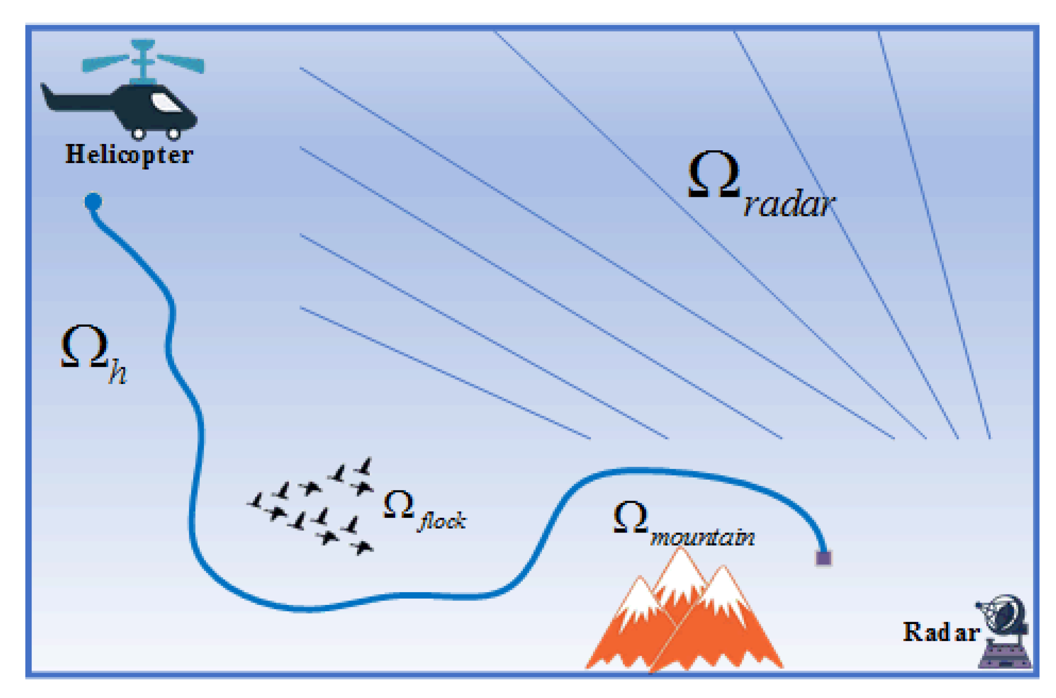
The four elements: UH, radar, stationary mountain, and flock of birds making random movements in the low airspace range are included in the complex battlefield environment. In the process of raiding the radar, UH not only needs to avoid being detected by the radar, but also needs to avoid mountains and bird flocks to ensure its own safety. In this section, the battlefield environment is numerically analysed and modelled.
3.1. Environmental Overview
The battlefield environment that UH faces when performing raid missions in low airspace is shown in
Figure 1.
,
,
, and
represent the helicopter flight area, the area of the static obstacle mountain, the area of the dynamic obstacle flock of birds, and the radar coverage area, respectively. The complex battlefield environment is replaced by
, and
represents any position in it. Then,
and
represent the horizontal position and flight altitude of the UH, respectively.
The static environment
contains the following sets:
where
represents the union operation in the set operation. The dynamic environment
contains the following sets:
where
indicates that the location area of the flock will change with time. In addition, the movement direction of the flock is random, and the dimension of its movement is consistent with UH. In this article, UH moves with eight degrees of freedom in
and the specific motion direction is shown in
Figure 2.
The safety radius R of UH is inviolable, and the safety radius
R is determined by the following factors:
where
represents the current position of UH.
Based on the above information, the passable condition
and impassable condition
of UH can be obtained as:
where
f(
x) represents the judgment function, and 0 and 1 represent movable and completely immovable, respectively.
means detected by radar.
3.2. Parameter Setting
It is assumed that UH needs to raid radar positions 50 km away. Therefore, the length of the experimental environment is set to 50 km, and the height is set to 1 km. Then, the radar position
can be expressed as:
The horizontal flight speed
of UH is 360 km/h, and the vertical flight speed
is 10 m/s. Then, the UH position
can be expressed as:
Because the horizontal speed and vertical speed of UH are not in the same order of magnitude, the safety radius
R of the UH should also be divided into two dimensions: horizontal and vertical. The UH safety radius can be set as:
The maximum attack distance of UH is 8 km. Assuming that the hit rate of UH in each attack is 100%. Then, the condition for UH to complete the raid task is that the distance
between UH and the radar is less than 8 km:
The maximum detection range of the radar is 45 km. Due to the influence of ground reflection clutter and detection angle, it is usually difficult for radar to detect low-flying targets. It is assumed that the radar detection probability formula is:
Combining the above information, the probability model of UH flight process detected by radar can be obtained as shown in
Figure 3.
In
Figure 3, the d-axis is the distance between the UH and the radar position, the h-axis is the flying height of the UH, and the i-axis is the probability of being detected by the radar. As can be seen from
Figure 3, UH can avoid radar detection by lowering the flying height. Combined with the probability map, it can be seen that within the range of the flight height
, the probability of being detected by the radar is not 100%, which creates an obstacle for UH to recognize environmental information, and is also one of the difficulties of this path planning experiment.
4. Path Planning Scheme in Dynamic Environment
In this section, we briefly describe the development of DRL and the DQN algorithm and make a series of improvements to the DQN algorithm. First, a goal-oriented dynamic reward function is designed to overcome the sparse reward problem existing in the traditional DQN algorithm, which can give appropriate rewards in time according to the state changes of UH. On this basis, a state-encoding method is designed to encode the environmental state faced by UH. Finally, with the encoded environment state as input, the SC-DQN algorithm is proposed.
4.1. Deep Reinforcement Learning
Reinforcement learning is a Markov decision process consisting of a quadruple , where and are the state space and action sets, is the state transition probability, and is the reward set. In the current state , the learner will select the action according to the policy and after executing the action. Then, it will further transfer to the next state according to the probability , and at the same time, receive the reward from the environment.
The combination of reinforcement learning and neural network has been studied in a previous work, but the algorithm performance is not good [
26]. It was not until the DQN algorithm was proposed that deep reinforcement learning was greatly developed [
27]. The success of the DQN algorithm is mainly attributed to the introduction of two mechanisms: experience replay and target network. Since the correlation between the samples is much larger than that of a simple reinforcement learning problem, experience replay can make the deep neural network converge to the same step size, which can make the gradient descent of the algorithm move in the same direction, thereby promoting the algorithm to converge. At the same time, random sampling of training samples from the experience pool can improve data utilization, thus effectively solving three problems: overcoming the correlation of empirical data, reducing the variance of parameter updates, and overcoming the non-stationary distribution problem [
28].
The DQN algorithm uses the Q-Learning algorithm [
29] to provide labelled samples to the neural network and then uses gradient descent to update the neural network parameters through back propagation. The update method of the Q-Learning algorithm is:
where
is the learning rate, which is used to control the proportion of future rewards in the learning process.
is the decay factor, which represents the decay of future rewards.
represents the reward after action
is performed. For formula (11), if each state
and action
are visited infinitely, and the decay factor
takes an appropriate value, then the
value will eventually converge to a fixed value. The convergence of Equation (11) has been proved in [
30]. The Q-Learning algorithm needs to generate a Q table to store the
value during the running process, and it needs to constantly read and write the
value to update the Q table.
The DQN algorithm uses a neural network to fit the update process of the Q-Learning algorithm. In the DQN algorithms, the state of the learner is used as input, and the
value corresponding to each action is used as output, such that the
value information is stored in the neural network node, namely:
where
represents the neural network parameters.
The loss function for the
value is defined in terms of mean squared error:
The in formula (13) is generated by the evaluate network, and is generated by the target value network. The parameters of the target value network are exactly the same as the evaluate network. When the algorithm updates a certain number of steps, the parameters of the evaluate network will be completely copied to the target network. The target value network can solve the problem of strong data dependence when a single network is updated, thus effectively promoting the convergence of the algorithm.
The training process uses the stochastic gradient descent algorithm to update the network parameters
:
in formula (14) is generated by the neural network calculation. Then, the DQN algorithm code is shown in Algorithm 1.
| Algorithm 1: DQN Algorithm |
Initialization: initialize training network parameter ω and target network parameter ω′, ω = ω′.
Iterative process:
Repeat (for each episode)
Initialization state s
Repeat (for each step)
Select action a based on the ε—greedy policy
Perform action a to obtain reward r and next state s′
Store transition (s,a,r,s′) in the experience memory
Sample random mini batch (s,a,r,s′) from the experience memory
Loss function L(ω) is obtained
Updating network parameters
s = s′
End Repeat (s′ is the terminated state)
End Repeat (end of the training) |
4.2. Reward Function Design
The setting of the reward function is an important part of the reinforcement learning algorithm, and a reasonable reward setting can promote the rapid convergence of the algorithm [
31]. However, in the traditional reinforcement learning algorithm, the learner is rewarded when completing the task, and there is no reward in other states. This kind of reward can easily lead to the sparse reward problem in the face of complex environments [
32]. In a complex environment, the state space is usually large, and the learner will face many non-feedback states before completing the task. Since the effective reward cannot be obtained in time, the algorithm will be difficult to converge. Aiming at this problem, this paper designs a goal-guided reward function whose specific expression is (15), where
is the reward coefficient, and
and
are the distances between the UH and the radar target in the current state and the next state, respectively.
is a constant greater than the maximum distance between the UH and the target position. The calculation methods of
and
refer to formula (9).
It can be seen from Equation (16) that the reward will be related to the distance between the UH and the target in real time. Whenever the position of the UH changes, if it is closer to the target, a positive reward can be obtained. Otherwise, there will be punishment (negative reward). At the same time, when the UH is far away from the target, the disciplinary effect of the negative reward is stronger, and the UH will quickly approach the target point of the constraint of the negative reward. As the distance between the UH and the target decreases, the constraint ability of the negative reward gradually weakens, and the incentive effect of positive reward increases. UH will explore sub-optimal actions at the same time when approaching the target point (taking sub-optimal actions will not be severely punished), so as to effectively seek the optimal path.
Equation (15) is the reward of UH when it satisfies the passable condition . When UH meets the impassable condition , that is, when the distance between UH and the obstacle is less than the safety radius , the reward value is −1000. Then, the system exits and starts learning again. In addition, when the distance between the UH and the target radar is less than 8 km, the task can be regarded as completed. At this time, the reward is 1000, and the system will also exit and start learning again.
To sum up, the reward function designed this time can generate dynamic rewards in real time in combination with environmental information. The dynamics of rewards are mainly manifested in two aspects. First, the rewards are generated in real-time as the UH interacts with the environment, which makes the reward no longer sparse. Second, the numerical value of the reward is not fixed; it will change with the movement of the learner. This change guides the UH to move in the correct direction, which further facilitates algorithm convergence. Based on the above analysis, UH can optimize the search according to the continuously estimated environmental cost information to make the reward accumulation process smoother. Since the reward situation is related in real time to the task goal, it is called a goal-directed reward function.
4.3. Status Code
The conventional DQN algorithm takes the learner’s location information as input, and after repeated interactive learning with the environment, it can learn to take correct actions at the corresponding location, so as to reach the destination smoothly. This input method theoretically requires the learner to traverse all the positions to complete the training. However, in a complex environment, the location space is relatively large; thus, the learning efficiency of the algorithm is low. Conversely, the training result of this input method is to enable the learner to make correct decisions at the corresponding position, but when the environmental state of the corresponding position changes, it is difficult for the learner to deal with this situation. Therefore, this input method is difficult to perform the path planning task of UH in complex dynamic environment.
The premise of path planning in the dynamic environment is that learners can accurately identify the current environment state in real time. If the next move may encounter an obstacle, the learner should accurately identify the location of the obstacle, so as to judge the current state and make the correct decision to avoid the obstacle. In order for UH to accurately judge the current environment state in real time, a state encoder is designed to encode the surrounding environment information detected by UH, thereby changing the input method of the traditional DQN algorithm.
As shown in
Figure 4, in a grid environment, assuming that the UH can perceive the surrounding environment information (which is easy to implement for the UH equipped with various sensors). First, we propose features for the grid adjacent to the current position of UH, so as to accurately determine the existence of surrounding obstacles. Then, we encode the adjacent positions, so as to accurately convert the environmental information into digital codes. In this process, we use 1 or 0 to represent the presence of obstacles or the absence of obstacles, respectively. This encoding is concise and efficient. Finally, we use the encoded information as the input of the algorithm. Since the encoded environmental state is composed of numbers 0 and 1, it can be directly used as the input of the algorithm without decoding. The algorithm can judge the existence of obstacles in the surrounding environment by distinguishing between 0 and 1, so as to make the correct decision.
By the above coding scheme, the traditional input of learner location information is converted to the input of learner state information. When the algorithm takes the location information of the learner as the input, it completes the division of the environment state space based on the location information. As the simulation accuracy improves, the learner’s location information increases, which means that the environment state space also expands. This increases the training burden of the algorithm. However, when the algorithm takes the learner’s state information as input, it completes the division of the environment state space based on the existence of surrounding obstacles. Since the distribution of surrounding obstacles is limited and will not increase with the improvement of simulation accuracy, the environment state space is also limited. Compared with traditional methods, our scheme can be regarded as compressing the state space, thus effectively reducing the training burden of the algorithm.
Combined with the battlefield environment, it can be seen from
Figure 2 that UH moves with eight degrees of freedom in the environment. Assuming that obstacles may be encountered in all eight directions, there will be 2
8 situations. It can be encoded by Boolean value (true is represented by 1 and false is represented by 0):
In formula (16), and the action directions of UH are corresponding, where means that there is no obstacle in this direction to pass, and means that there is an obstacle in this direction that is impassable. Using the encoded as the algorithm input, the UH after training can make correct decisions according to the current environment state, so as to complete the obstacle avoidance task, and can complete the local path correction when the position of the obstacle changes.
4.4. State-Coded Deep Q-Network
Combined with the idea of the above reward function and the state-coding scheme, the design of the UH path planning algorithm in the dynamic environment is completed. The algorithm model is shown in
Figure 5.
It can be seen from
Figure 5 that when the algorithm is executed, the state information of the surrounding environment of the learner is extracted, and then the surrounding environment state is sequentially encoded by the state encoder; then, the encoded
is used as the input. After the algorithm outputs the
values of different actions, the action
with the largest
value is selected according to the ε-greedy strategy and is executed. Then, the environment state changes and the next state
is obtained. At this time, the environment rewards
for action
according to the reward function, and the complete quaternary information group
is obtained. The quaternary information group will be stored in the experience pool. After the experience pool stores a certain scale of data, it will be randomly sampled for learning. In the process of sampling learning, the current state
of the learner will be used as the input of Evaluate Net to obtain the actual value
, and the next state
of the learner will be used as the input of Target Net to obtain the estimated value
. Next,
,
and reward
are used as the input of the loss function to obtain the mean square error, and the stochastic gradient descent method is used to update the Evaluate Net, thus as the action selection strategy of the SC-DQN algorithm is optimized. The input state
is encoded in combination with the motion direction of the UH; thus, the input and output of the network are dimensionally consistent. Therefore, the deep learning network used by the SC-DQN algorithm has symmetric properties, which makes the network structure more stable.
5. Simulation Experiment
Scenario 1, Scenario 2 and Scenario 3 are used to verify the performance of the SC-DQN algorithm. In Scenario 1, the flock of birds in
Figure 1 does not exist, and the impassable areas in the environment are the radar coverage area and the location of the mountains. Then, the passable condition of UH is Equation (4), and the impassable condition is:
The position of the mountain in Scenario 1 is , and the height of the mountain relative to the ground is 0.15 km. Compared to Scenario 1, the position of the mountains is changed in Scenario 2. The position of the mountain was adjusted to , which is used to verify the path correction ability of the algorithm.
In Scenario 3, a flock of birds is introduced into the environment. The horizontal movement speed of the flock is 36 km/h, and the vertical movement speed is 1 m/s because the movement of the flock of birds is relatively random, and it is usually accustomed to moving in a low airspace range. Therefore, we limit the movement range of the flock of birds to a low airspace range with an altitude of no higher than 0.2 km. The flock of birds will appear at the beginning of the mission, the location is random, and the movement direction of the flock at any time is also random.
In order to ensure the validity of the experiment, all experiments must be carried out in the same environment. This experimental environment code is written in Python language based on the PyCharm platform, and the neural network is built with the help of the Tensorflow-2.6.0 toolkits. All experiments were performed on the same computer with twelve Intel(R) Core (TM) i7-8700 CPU @ 3.20 GHz processors and one NVIDIA GeForce GT 430 GPU, and the RAM is 16 GB.
5.1. Algorithm Parameter Selection
The learning rate
and batch size are two important parameters in the SC-DQN algorithm. In order to select suitable parameters, we compared the convergence of the SC-DQN algorithm under different values. The experiment was carried out in Scenario 1. During the experiment, if UH completes the raid task, it will obtain one point; if not, it will not score. We take the score of UH’s last 100 tasks as an indicator to measure the performance of the algorithm. During the experiment, every time UH completes the task or fails the task, the system will exit and restart the training, which represents the end of an episode. The experimental results are shown in
Figure 6 and
Figure 7. The results in
Figure 6 are obtained by averaging the data of 10 independent experiments, which reduces experimental error.
Figure 6 shows score of the proposed SC-DQN algorithm with different learning rates, in which the learning rates are 0.001, 0.005, 0.01, 0.05 and 0.1. As we can see, the learning rate affects the value of the score during the training of our algorithm. The reason is that the learning rate represents the learning step length of realizing the convergence of the algorithm. The higher the learning rate, the more the learning effect is preserved, and the training is faster, but it is easy to miss the global optimum of the learning process, which causes oscillation. Then, the smaller the learning rate, the slower the training. According to our experimental results, the learning rate 0.05 has the best performance in our simulation scenario. Its learning speed is acceptable, and it can quickly lead to the convergence of the algorithm.
Figure 7 shows the learning loss of the proposed SC-DQN algorithm with different batch size, in which the batch size values are 8, 16, 32 and 64, respectively. As we can see, the batch size affects the value of the loss with the increase in learning episodes. The batch size affects the efficiency of sampling when the algorithm performs experience replay. If the batch size is small, it will bring a large variance, which will slow down the convergence of the SC-DQN algorithm. Meanwhile, if the batch size is too large, it might lead to the convergence of the algorithm to the local optimal solution point. Therefore, the batch size should take a suitable and appropriate value. According to our experimental results, the batch size should be set as 32. In addition, it can be seen that the learning loss after training has dropped to a small value and remains stable. This proves that our algorithm can achieve convergence in Scenario 1.
In addition to the learning rate and batch size, there are influences from other parameters in the experiment: The larger the decay factor , the more attention is paid to past experience, and the smaller the value, the more attention is paid to current returns. If the exploration factor is too large, the algorithm will tend to maximize the current profit and lose the motivation of exploration; thus, it may miss the bigger profit in the future. There are too few hidden layers and neurons in the hidden layer to fit the data well, and too many to learn effectively. Based on the above experimental results and past experience, the final parameters are set as follows: the learning rate is 0.05, the decay factor is 0.9, and the exploration factor is 0.9. The input layer and output layer of the neural network are both eight neurons, and the hidden layer is two identical fully connected networks, with 16 neurons set in each layer. The experience pool size is 1600, and the batch size is 32. Since the traditional sparse reward method is difficult to converge on the context of this experiment, the two algorithms both adopt the dynamic reward function designed in this paper as the reward method during the experiment. Our proposed algorithm only improves the input method of the traditional algorithm, which does not change the convergence process of the original algorithm. Therefore, it is reasonable for both algorithms to choose the same parameter settings for comparative experiments.
5.2. Global Path Planning and Obstacle Avoidance in Static Environment
Figure 8 shows the path length of the DQN algorithm and SC-DQN algorithm with training episodes in Scenario 1, in which both algorithms eventually converge. As we can see, the SC-DQN algorithm converges faster than the DQN algorithm, and the path length is shorter than the DQN algorithm. The path lengths after the convergence of the two algorithms are still not stable enough. The reason is that the existence of the exploration factor
makes UH not always choose the optimal strategy, which leads to the appearance of oscillation.
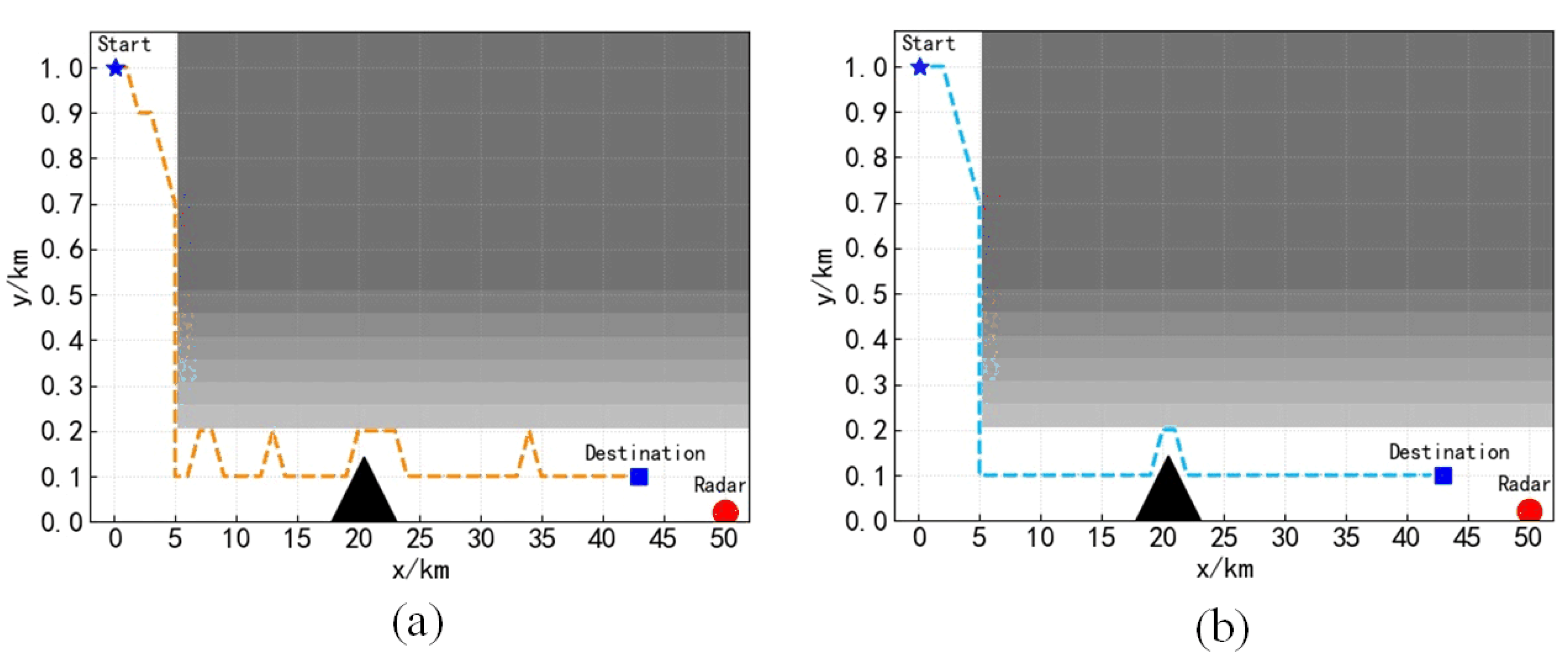
Using the trained algorithm to conduct a path planning test in scenario 1,
Figure 9 is obtained. It can be seen from
Figure 9 that both algorithms can plan a safe path in Scenario 1 and successfully avoid the mountains in the environment. By comparing
Figure 9a,b, it can be seen that the path planned by the DQN algorithm is not smooth enough.
Figure 10 and
Figure 11 show the path length and path smoothness for DQN and SC-DQN. In order to make the obtained path length more accurate, we averaged the results of 10 experiments to obtain
Figure 10. The error generated during data processing is calculated by the standard deviation formula:
As we can see, the path planned by the SC-DQN algorithm is shorter and smoother than the path planned by the DQN algorithm. In order to verify the ability of the algorithm to correct the path, the trained network for the path planning test was used in Scenario 2 and obtain
Figure 12.
Figure 12 shows the path planning test results in Scenario 2. It can be seen from the figure that when the position of the mountain is changed, the DQN algorithm still flies according to the original planned path and fails to avoid the mountain, while the SC-DQN algorithm successfully corrected the local paths and avoided the mountain.
5.3. Local Path Correction and Obstacle Avoidance in Dynamic Environment
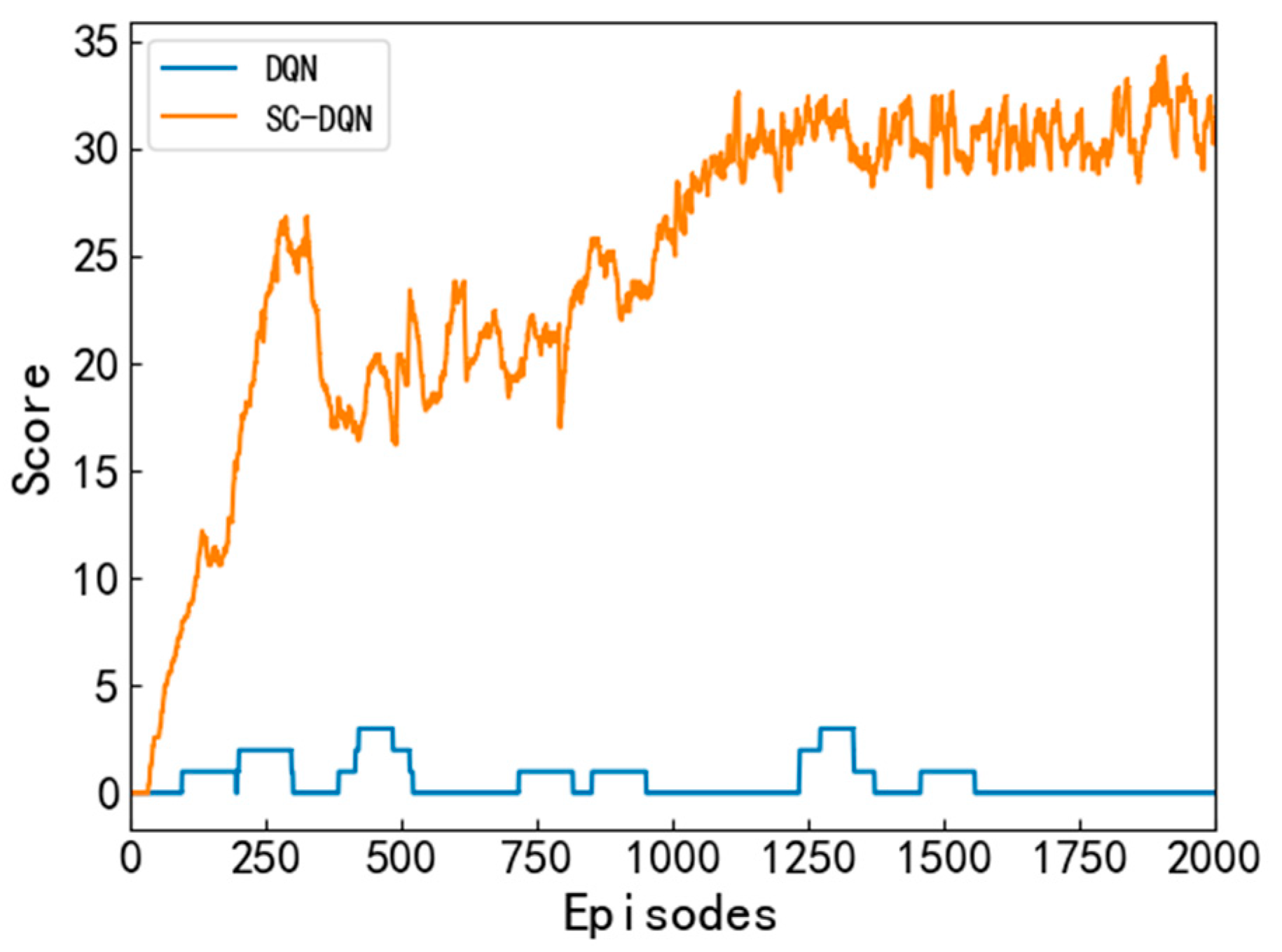
The two algorithms are retrained in Scenario 3, and the algorithm scores are shown in
Figure 13. As we can see, the SC-DQN algorithm can still converge smoothly after training in Scenario 3, but the DQN algorithm is difficult to converge.
To further verify the performance of the SC-DQN algorithm, we conducted a large number of paths planning test experiments in Scenario 3. In Scenario 3, since the initial positions and movement directions of the flock of birds were randomly generated, it is unrealistic to show all the test results. Therefore, we only selected the experimental results of four representative special encounter scenarios for display and analysis, as shown in
Figure 14. The blue line in the figure represents the complete flight path of the UH, while the purple line only represents the movement trajectory of the moment when the flock encounters the UH.
In
Figure 14a, the movement state of the flock is from position 1 to position 2. When UH encounters a flock of birds at position 1, it immediately converts the movement direction
to
. However, the birds still interfere with the flight of UH after moving from position 1 to position 2. Therefore, UH performs path correction again. UH converts the movement direction from
to
, thus successfully avoiding the flock of birds.
In
Figure 14b, the movement state of the flock of birds is from position 3 to position 4. When the UH encounters a flock of birds at position 3, it changes the original movement direction
but switches to the movement direction
. After the flock of birds moves from position 3 to position 4 to give way to the travel path, UH continues to move in the direction of
.
In
Figure 14c, the movement state of the flock of birds is from position 5 to position 6. When UH encounters a flock of birds at position 5, it converts the original movement direction
to direction
to avoid the flock. After the flock of birds moves from position 3 to position 4, it still interferes with the UH’s movement in the movement direction
. Thus, the UH continues to move forward in the movement direction
and moves in the movement direction
only after flying to the safe area.
In
Figure 14d, the movement state of the flock of birds is from position 7 to position 8. When the UH encounters a flock of birds at position 7 in the process of descending, in order to avoid the flock, the UH converts the original movement direction
to the movement direction
. The flock of birds moves from position 3 to position 4 without further disturbing the UH; thus, the UH continues to move forward using the movement direction
.
5.4. Analysis and Discussion
Through the simulation experiments in
Section 4.2 and
Section 4.3, the proposed SC-DQN algorithm is tested in static and dynamic environments, respectively. The experimental scheme fully takes into account the various emergencies that the UH may encounter during the mission. The experimental results show that the SC-DQN algorithm can complete the global path planning, obstacle avoidance and local path correction tasks of UH in a complex dynamic environment, and can handle various emergencies, including the sudden appearance of bird flocks with uncertain motion states.
In
Section 5.2, a comparative analysis of
Figure 9 and
Figure 12 is carried out. Although the traditional DQN algorithm can help UH to complete the path planning and obstacle avoidance tasks in a static environment, it cannot correct the path in time when the position of the obstacle changes because the UH trained by the DQN algorithm makes decisions by identifying the location information about the environment. Once the environmental information changes, the decision of the corresponding location should also change, but the UH trained by the DQN algorithm does not effective identify these changes. Different from the DQN algorithm, the SC-DQN algorithm directly uses the environmental state as input for learning. Although the position of the obstacle has changed, the state that UH faces when encountering an obstacle will not change. Therefore, the trained UH by the SC-DQN algorithm is still able to accurately identify changes in the environmental state, thereby making corrections to the planned path. In addition, it can be seen from
Figure 10 and
Figure 11 that the path planned by the DQN algorithm is not smooth enough, and there is a certain degree of oscillation, which is unfavourable for the UH flight. We know that there are suboptimal strategies in different positions in the environment to a certain extent. For the DQN algorithm, it takes a huge cost to explore the optimal strategy for each position. However, the environmental state faced is relatively limited for the SC-DQN algorithm, such that the optimal strategy in the corresponding state can be explored more quickly. Therefore, after the same degree of training, the path planned by the SC-DQN algorithm is smoother.
In
Section 5.3, due to the introduction of a flock of birds with random movements in the environment, the environmental state at the same location is changing, which is unacceptable for the DQN algorithm. Therefore, the DQN algorithm is difficult to converge in this dynamic environment. For the SC-DQN algorithm, the movement of the flock of birds does not affect the UH’s recognition of the environmental state; thus, the SC-DQN algorithm can still converge smoothly. It can be seen from
Figure 14 that when encountering a flock of birds in different scenarios, the UH trained by the SC-DQN algorithm can correct the path in time to avoid the flock of birds. This shows that that SC-DQN algorithm can handle the avoidance problem of dynamic obstacles well, which proves the security of the algorithm.
In addition, during the experiment, both the DQN algorithm and the SC-DQN algorithm adopt the goal-guided dynamic reward function designed in
Section 3.2 as the reward rule. Through many experimental tests, this reward method can give the correct reward feedback to the algorithm in time, guide the UH to quickly approach the target, effectively overcome the sparse reward problem existing in traditional reinforcement learning algorithms, and promote algorithm convergence.
6. Conclusions
In this paper, a path planning algorithm that can help UH to perform flight missions in complex low airspace environments is proposed. The numerical analysis of the UH low airspace flight environment is carried out, and the mathematical modelling of the low airspace environment is completed. In order to improve the sparse reward problem faced by reinforcement learning, a goal-guided dynamic reward function that conforms to the characteristics of the environment is designed to facilitate the algorithm to converge quickly in a large state space. At the same time, the environment state faced by UH is encoded by binary Boolean expression, and the SC-DQN algorithm is proposed. The simulation results show that the SC-DQN can help UH safely and effectively avoid various obstacles in a complex low airspace environment and successfully complete the raid task. In brief, the proposed SC-DQN algorithm is a complete path planning algorithm that integrates global path planning, obstacle avoidance and local path correction. Our coding scheme requires accurate extraction of environmental information to determine the location of obstacles, which is easy in simulation experiments but is not easy in practical applications. Extracting environmental features requires a large number of sensors to work together, which is a challenging task. Therefore, our algorithm may encounter some difficulties when applied in real-time.
In future works, further enrichment of the input information of deep reinforcement learning algorithms can be considered. More environmental information input can prompt the algorithm to make more favourable decisions for the learner. Using the intention recognition mechanism [
33] to determine the intent of moving obstacles is a potential research hotspot. Incorporating intent recognition results into algorithmic input can help algorithms make better coping decisions. Conversely, accurately identifying and judging the status of obstacles is also a problem worthy of attention, which can make the state-encoding process much simpler. Therefore, the use of graph classifiers [
34] to identify obstacles is another potential research hotspot.
Author Contributions
Conceptualization, J.Y.; methodology, J.Y.; software, J.Y.; validation, J.Y., X.L. and J.J.; formal analysis, J.Y.; investigation, X.L.; resources, X.L., Y.Z., Y.W. and Y.L.; data curation, X.L.; writing original draft preparation, J.Y.; writing—review and editing, J.Y., X.L, Y.Z., J.J., Y.W. and Y.L.; visualization, J.Y. and J.J.; supervision, X.L., Y.Z. and Y.W.; project administration, X.L.; funding acquisition, Y.Z. and Y.L. All authors have read and agreed to the published version of the manuscript.
Funding
This research was funded by the National Natural Science Foundation of China, grant number 62071483, and the National Natural Science Foundation of China, grant number 61602505.
Institutional Review Board Statement
Not applicable.
Informed Consent Statement
Not applicable.
Data Availability Statement
The data used to support the findings of this study are available from the corresponding author upon request.
Conflicts of Interest
The authors declare that they have no conflict of interest or personal relationships that could have appeared to influence the work reported in this paper.
References
- Ni, S.; Liu, Z.; Huang, D.; Cai, Y.; Wang, X.; Gao, S. An application-orientated anti-collision path planning algorithm for unmanned surface vehicles. Ocean Eng. 2021, 235, 109298. [Google Scholar] [CrossRef]
- Qi, J.; Yang, H.; Sun, H. MOD-RRT*: A Sampling-Based Algorithm for Robot Path Planning in Dynamic Environment. IEEE Trans. Ind. Electron. 2020, 68, 7244–7251. [Google Scholar] [CrossRef]
- Sun, P.; Guo, Z.; Lan, J.; Hu, Y.; Baker, T. ScaleDRL: A Scalable Deep Reinforcement Learning Approach for Traffic Engineering in SDN with Pinning Control. Comput. Netw. 2021, 190, 107891. [Google Scholar] [CrossRef]
- Yu, X.; Li, C.; Zhou, J.F. A constrained differential evolution algorithm to solve UAV path planning in disaster scenarios. Knowl.-Based Syst. 2020, 204, 106209. [Google Scholar] [CrossRef]
- Zhang, J.; Xia, Y.; Shen, G. A Novel Learning-based Global Path Planning Algorithm for Planetary Rovers. Neurocomputing 2019, 361, 69–76. [Google Scholar] [CrossRef] [Green Version]
- Wang, N.; Jin, X.; Er, M.J. A multilayer path planner for a USV under complex marine environments. Ocean Eng. 2019, 184, 1–10. [Google Scholar] [CrossRef]
- Naeem, W.; Irwin, G.W.; Yang, A. COLREGs-based collision avoidance strategies for unmanned surface vehicles. Mechatronics 2012, 22, 669–678. [Google Scholar] [CrossRef]
- Ammar, A.; Bennaceur, H.; Chaari, I.; Koubâa, A.; Alajlan, M. Relaxed Dijkstra and A* with linear complexity for robot path planning problems in large-scale grid environments. Soft Comput. 2016, 20, 4149–4171. [Google Scholar] [CrossRef]
- Singh, Y.; Sharma, S.; Sutton, R.; Hatton, D.; Khan, A. A constrained A* approach towards optimal path planning for an unmanned surface vehicle in a maritime environment containing dynamic obstacles and ocean currents. Ocean Eng. 2018, 168, 187–201. [Google Scholar] [CrossRef] [Green Version]
- Wang, H.; Qi, X.; Lou, S.; Jing, J.; He, H.; Liu, W. An Efficient and Robust Improved A* Algorithm for Path Planning. Symmetry 2021, 13, 2213. [Google Scholar] [CrossRef]
- Wu, P.; Xie, S.; Liu, H.; Peng, Y.; Li, X.; Luo, J. Autonomous obstacle avoidance of an unmanned surface vehicle based on cooperative manoeuvring. Ind. Robot 2017, 44, 64–74. [Google Scholar] [CrossRef]
- Shorakaei, H.; Vahdani, M.; Imani, B.; Gholami, A. Optimal cooperative path planning of unmanned aerial vehicles by a parallel genetic algorithm. Robotica 2016, 34, 823–836. [Google Scholar] [CrossRef]
- Ul Hassan, N.; Bangyal, W.H.; Ali Khan, M.S.; Nisar, K.; Ag. Ibrahim, A.A.; Rawat, D.B. Improved Opposition-Based Particle Swarm Optimization Algorithm for Global Optimization. Symmetry 2021, 13, 2280. [Google Scholar] [CrossRef]
- Wei, L.; Li, Z.; Li, L.; Wang, F.-Y. Parking Like a Human: A Direct Trajectory Planning Solution. IEEE Trans. Intell. Transp. Syst. 2017, 18, 3388–3397. [Google Scholar] [CrossRef]
- Tutsoy, O.; Brown, M. Chaotic dynamics and convergence analysis of temporal difference algorithms with bang-bang control. Optim. Control Appl. Methods 2016, 37, 108–126. [Google Scholar] [CrossRef]
- Suarez, J.; Du, Y.; Isola, P.; Mordatch, I. Neural mmo: A massively multiagent game environment for training and evaluating intelligent agents. arXiv 2019, arXiv:1903.00784. [Google Scholar] [CrossRef]
- Chang, L.; Shan, L.; Jiang, C.; Dai, Y. Reinforcement based mobile robot path planning with improved dynamic window approach in unknown environment. Auton. Robot. 2021, 45, 51–76. [Google Scholar] [CrossRef]
- Chen, C.; Chen, X.Q.; Ma, F.; Zeng, X.-J.; Wang, J. A knowledge-free path planning approach for smart ships based on reinforcement learning. Ocean Eng. 2019, 189, 106–299. [Google Scholar] [CrossRef]
- Tutsoy, O.; Brown, M. Reinforcement learning analysis for a minimum time balance problem. Trans. Inst. Meas. Control 2016, 38, 1186–1200. [Google Scholar] [CrossRef]
- Mnih, V.; Kavukcuoglu, K.; Silver, D.; Rusu, A.A.; Veness, J.; Bellemare, M.G.; Graves, A.; Riedmiller, M.; Fidjeland, A.K.; Ostrovski, G.; et al. Human-level control through deep reinforcement learning. Nature 2015, 518, 529–533. [Google Scholar] [CrossRef]
- Cheng, Y.; Zhang, W. Concise deep reinforcement learning obstacle avoidance for underactuated unmanned marine vessels. Neurocomputing 2018, 272, 63–73. [Google Scholar] [CrossRef]
- Wu, X.; Chen, H.; Chen, C.; Zhong, M.; Xie, S.; Guo, Y.; Fujita, H. The autonomous navigation and obstacle avoidance for USVs with ANOA deep reinforcement learning method. Knowl.-Based Syst. 2020, 196, 105201. [Google Scholar] [CrossRef]
- Huang, R.; Qin, C.; Li, J.L.; Lan, X. Path planning of mobile robot in unknown dynamic continuous environment using reward-modified deep Q-network. Optim. Control Appl. Methods 2021. [Google Scholar] [CrossRef]
- Guo, S.; Zhang, X.; Du, Y.; Zheng, Y.; Cao, Z. Path planning of coastal ships based on optimized DQN reward function. J. Mar. Sci. Eng. 2021, 9, 210. [Google Scholar] [CrossRef]
- Xie, R.; Meng, Z.; Wang, L.; Wu, Z. Unmanned aerial vehicle path planning algorithm based on deep reinforcement learning in large-scale and dynamic environments. IEEE Access 2021, 9, 24884–24900. [Google Scholar] [CrossRef]
- Tsitsiklis, J.; Van Roy, B. An analysis of temporal-difference learning with function approximation (Technical Report LIDS-P-2322). Lab. Inf. Decis. Syst. 1996, 42, 674–690. [Google Scholar] [CrossRef] [Green Version]
- Chung, J. Playing Atari with Deep Reinforcement Learning. Comput. Ence 2013, 21, 351–362. [Google Scholar] [CrossRef]
- Li, J.; Chen, Y.; Zhao, X.N.; Huang, J. An improved DQN path planning algorithm. J. Supercomput. 2022, 78, 616–639. [Google Scholar] [CrossRef]
- Fan, J.; Wang, Z.; Xie, Y.; Yang, Z. A theoretical analysis of deep Q-learning. In Proceedings of the 2nd Conference on Learning for Dynamics and Control, Berkeley, CA, USA, 11–12 June 2020; pp. 486–489. [Google Scholar] [CrossRef]
- Tutsoy, O.; Brown, M. An analysis of value function learning with piecewise linear control. J. Exp. Theor. Artif. Intell. 2016, 28, 529–545. [Google Scholar] [CrossRef]
- Zheng, J.; Mao, S.; Wu, Z.; Kong, P.; Qiang, H. Improved Path Planning for Indoor Patrol Robot Based on Deep Reinforcement Learning. Symmetry 2022, 14, 132. [Google Scholar] [CrossRef]
- Memarian, F.; Goo, W.; Lioutikov, R.; Niekum, S.; Topcu, U. Self-supervised online reward shaping in sparse-reward environments. In Proceedings of the 2021 IEEE/RSJ International Conference on Intelligent Robots and Systems (IROS), Prague, Czech Republic, 27 September–1 October 2021; pp. 2369–2375. [Google Scholar] [CrossRef]
- Fang, Z.; López, A.M. Intention recognition of pedestrians and cyclists by 2d pose estimation. IEEE Trans. Intell. Transp. Syst. 2019, 21, 4773–4783. [Google Scholar] [CrossRef] [Green Version]
- Tomescu, M.A.; Jäntschi, L.; Rotaru, D.I. Figures of graph partitioning by counting, sequence and layer matrices. Mathematics 2021, 9, 1419. [Google Scholar] [CrossRef]
| Publisher’s Note: MDPI stays neutral with regard to jurisdictional claims in published maps and institutional affiliations. |
© 2022 by the authors. Licensee MDPI, Basel, Switzerland. This article is an open access article distributed under the terms and conditions of the Creative Commons Attribution (CC BY) license (https://creativecommons.org/licenses/by/4.0/).


