
GMS-RANSAC: A Fast Algorithm for Removing Mismatches Based on ORB-SLAM2

Abstract
:1. Introduction
2. Related Work
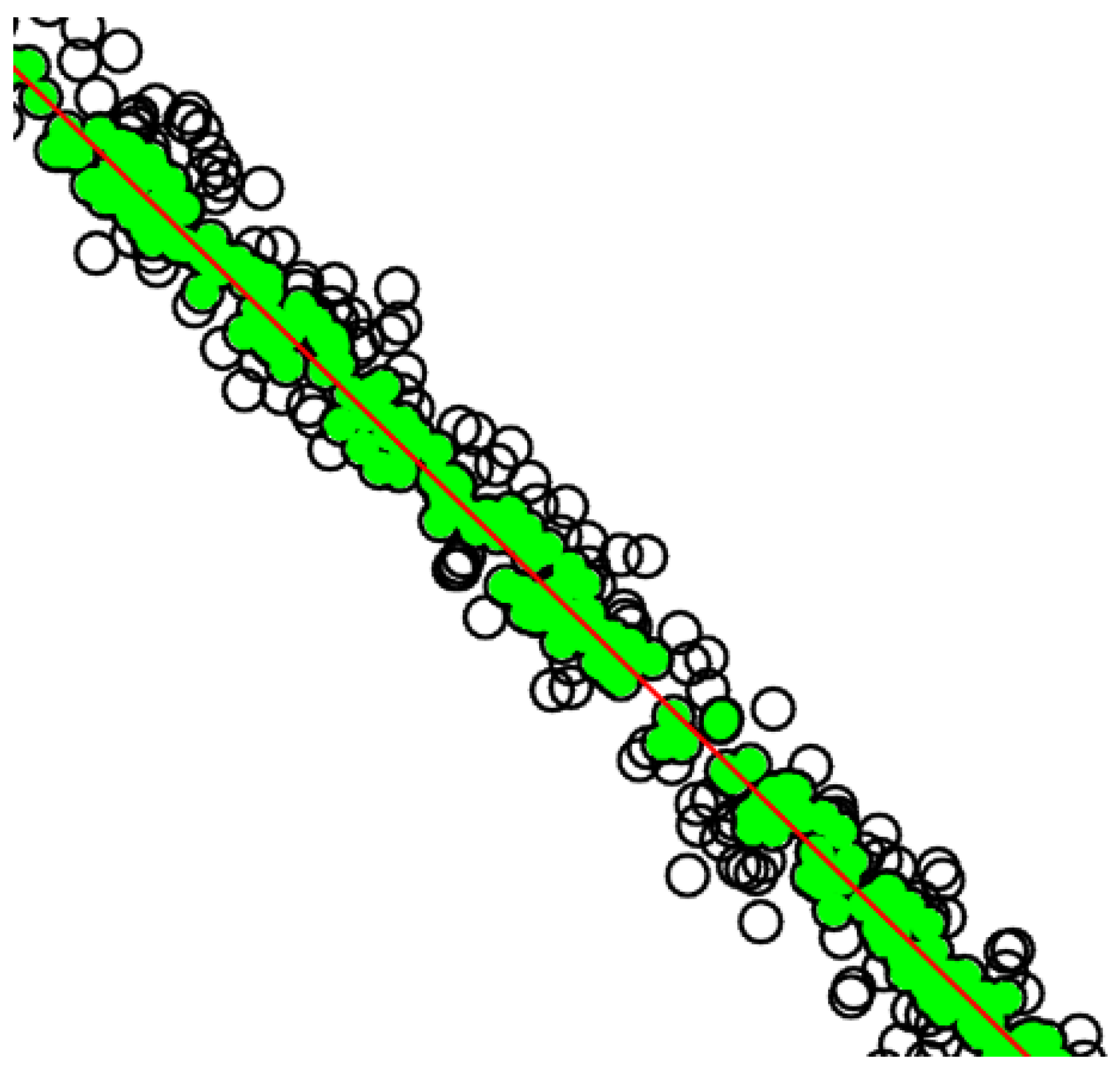
2.1. RANSAC
2.2. GMS
2.3. LPM
3. Methodology
3.1. Workflow of the Method
- (1)
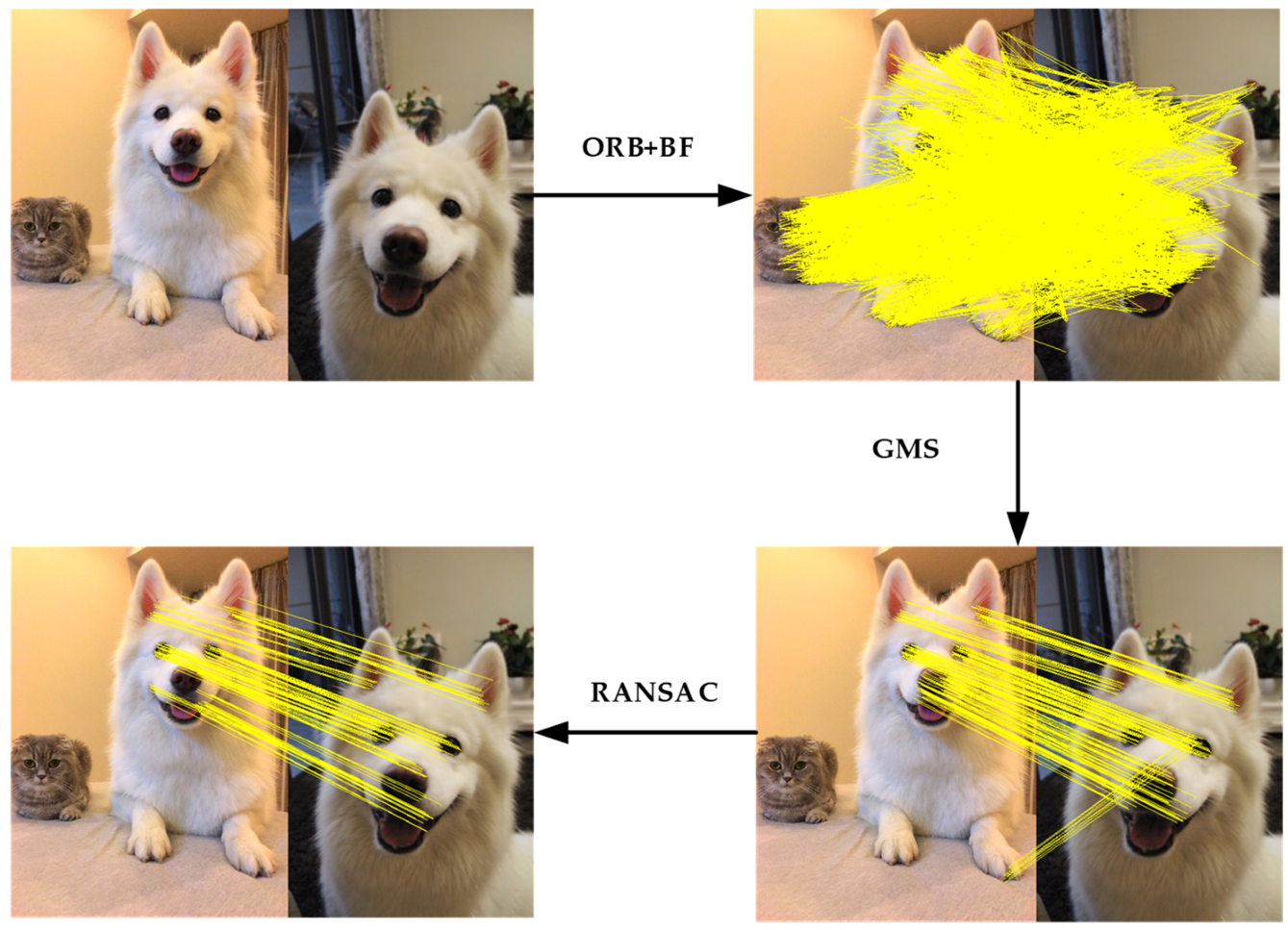
- Firstly, the ORB feature points of two images are extracted, respectively;
- (2)
- Then, the ORB features are matched by Hamming distance of descriptor;
- (3)
- Thirdly, the results of the previous step are roughly screened by GMS algorithm, which makes the number of matches greatly reduced;
- (4)
- Finally, the outliers are further removed by setting the random sampling consistency of the threshold.
3.2. GMS Mismatch Correction
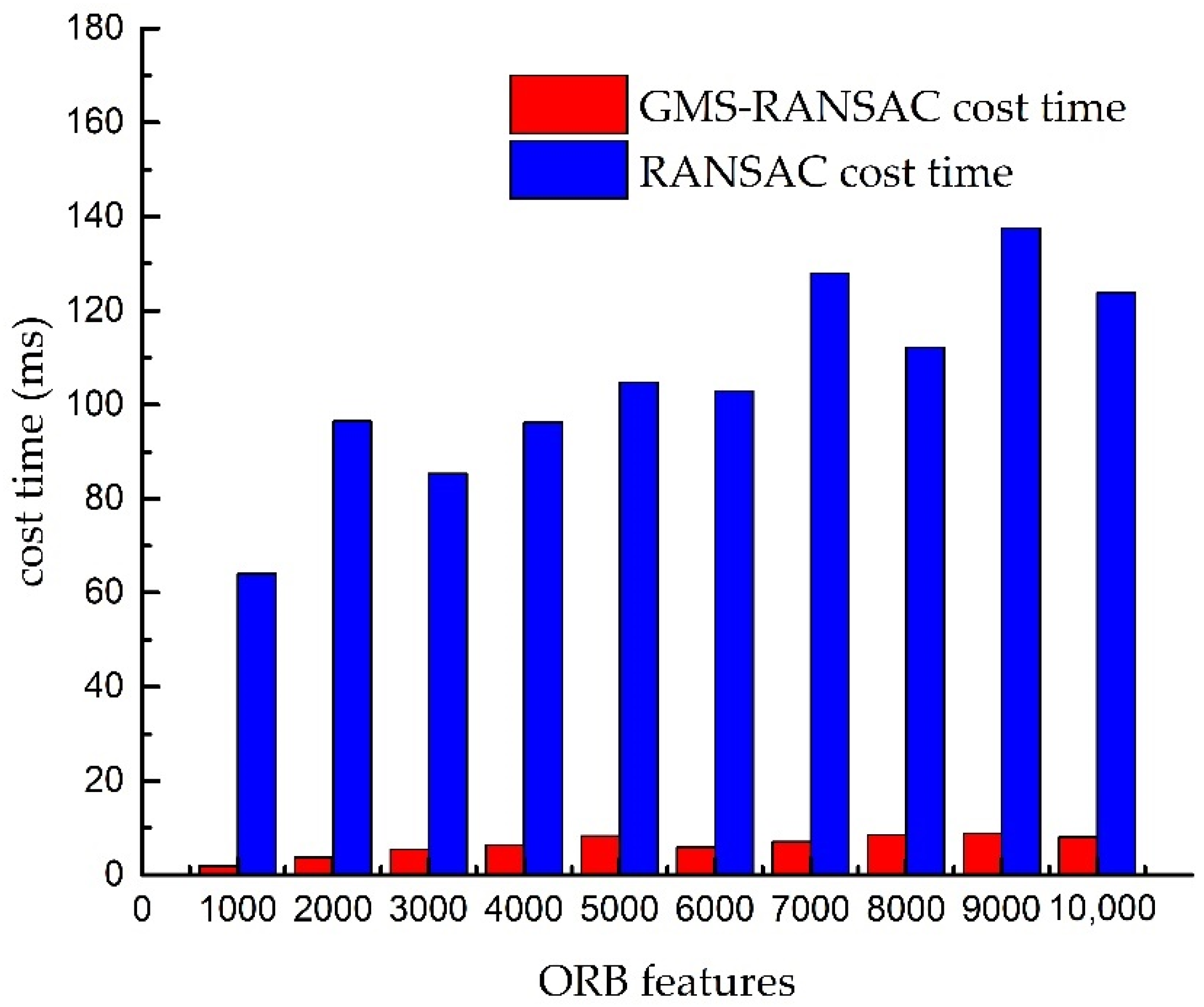
3.3. The Acceleration of RANSAC
4. Experiments
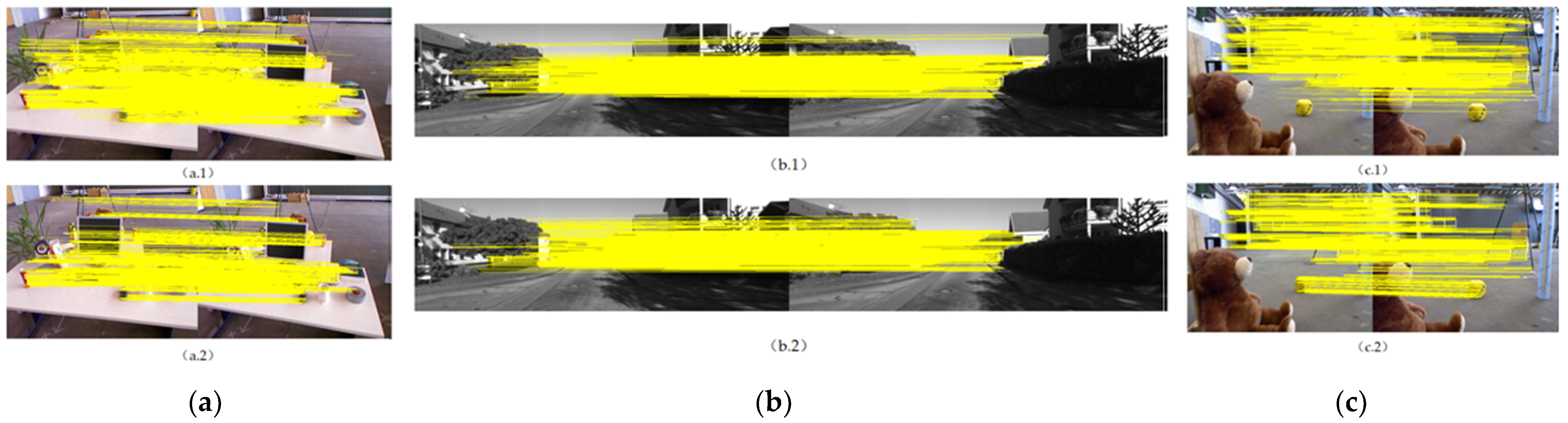
4.1. GMS-RANSAC for Correspondence Selection
4.1.1. Datasets and Metrics
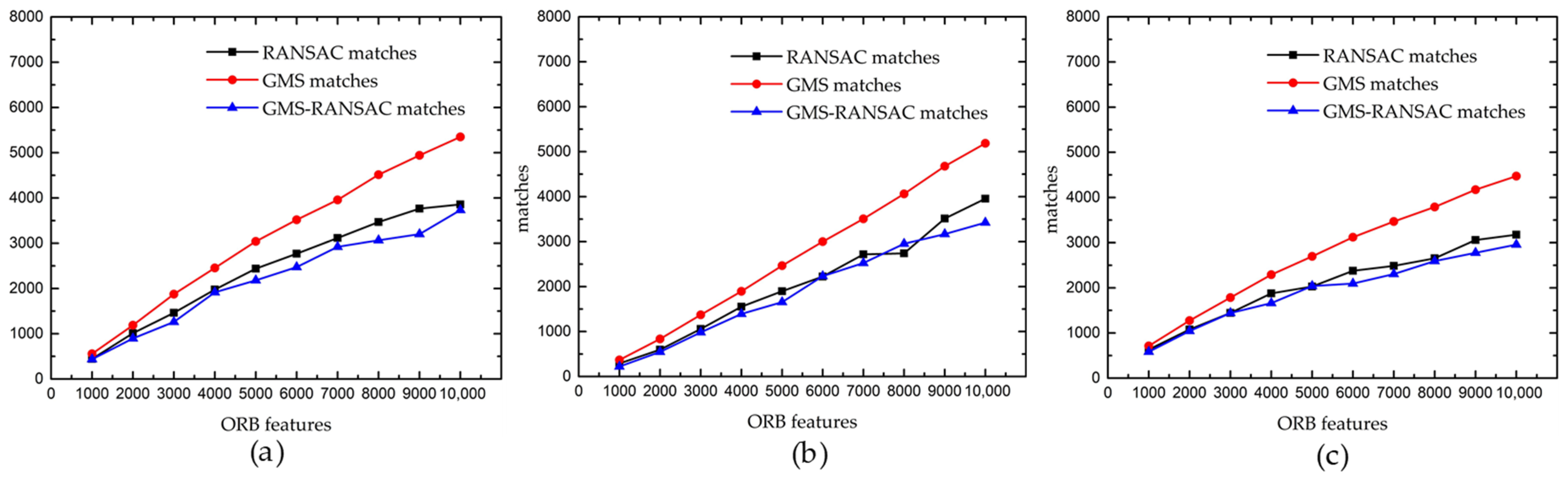
4.1.2. Experimental Results
4.1.3. Comparisons
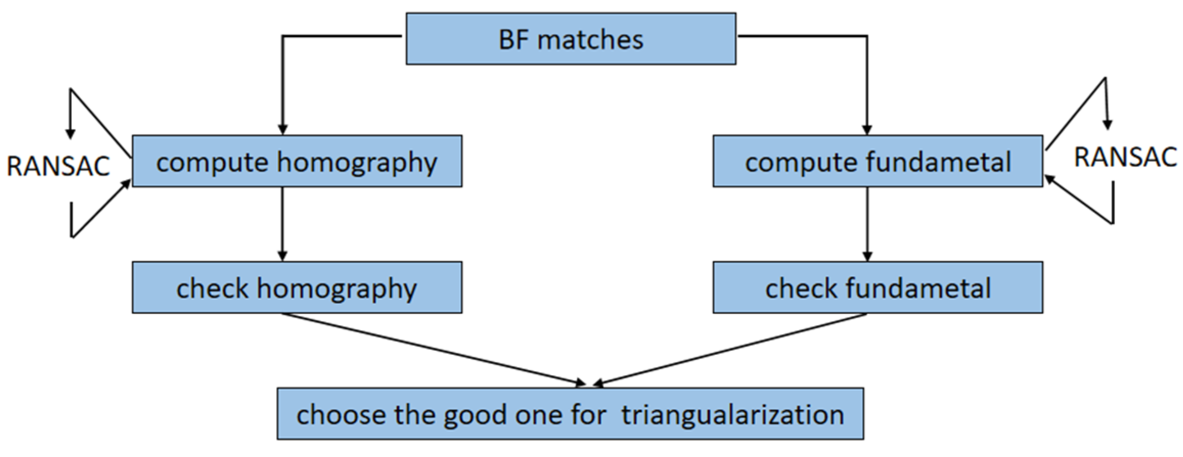
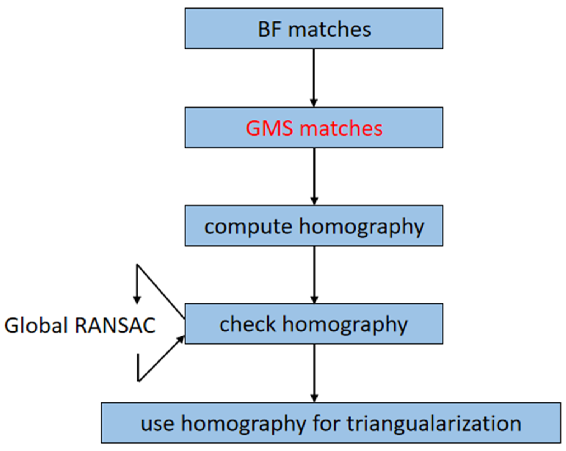
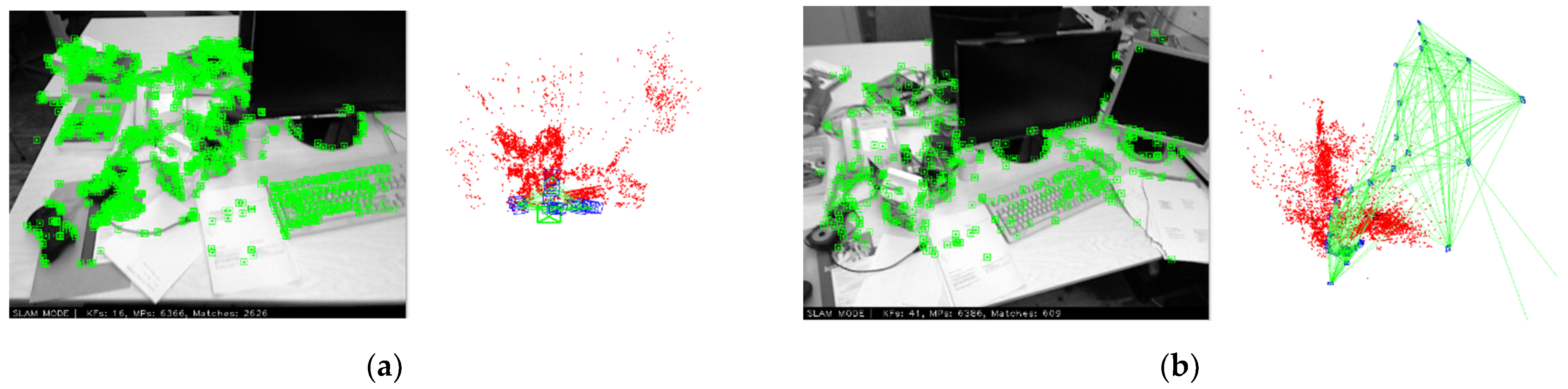
4.2. The New Initializer Based on ORB-SLAM2
4.2.1. Datasets and Metrics
4.2.2. Experimental Results
5. Conclusions
Author Contributions
Funding
Institutional Review Board Statement
Informed Consent Statement
Data Availability Statement
Acknowledgments
Conflicts of Interest
References
- Grisetti, G.; Stachniss, C.; Burgard, W. Improving Grid-based SLAM with Rao-Blackwellized Particle Filters by Adaptive Proposals and Selective Resampling. In Proceedings of the IEEE International Conference on Robotics & Automation, Barcelona, Spain, 18–22 April 2005. [Google Scholar]
- Davison, A.J.; Reid, I.D.; Molton, N.D.; Stasse, O. MonoSLAM: Real-time single camera SLAM. IEEE Trans. Pattern Anal. Mach. Intell. 2007, 29, 1052–1067. [Google Scholar] [CrossRef] [PubMed] [Green Version]
- Julier, S.J.; Uhlmann, J.K. New extension of the Kalman filter to nonlinear systems. In Signal Processing, Sensor Fusion, and Target Recognition VI; International Society for Optics and Photonics: Bellingham, WA, USA, 1997; Volume 3068, pp. 182–193. [Google Scholar]
- Klein, G.; Murray, D. Parallel Tracking and Mapping for Small AR Workspaces. In Proceedings of the IEEE & Acm International Symposium on Mixed & Augmented Reality, Cambridge, UK, 15–18 September 2008. [Google Scholar]
- Mur-Artal, R.; Montiel, J.M.M.; Tardos, J.D. ORB-SLAM: A Versatile and Accurate Monocular SLAM System. IEEE Trans. Robot. 2015, 31, 1147–1163. [Google Scholar] [CrossRef] [Green Version]
- Opdenbosch, D.V.; Steinbach, E. Collaborative Visual SLAM Using Compressed Feature Exchange. In Proceedings of the International Conference on Robotics and Automation, Pasadena, CA, USA, 19–23 May 2018; pp. 57–64. [Google Scholar]
- Bescós, B.; Fácil, J.; Civera, J.; Neira, J. DynSLAM: Tracking, Mapping and Inpainting in Dynamic Scenes. IEEE Robot. Autom. Lett. 2018, 3, 4076–4083. [Google Scholar] [CrossRef] [Green Version]
- Kim, T. Feature Detection Based on Significancy of Local Features for Image Matching. IEICE Trans. Inf. Syst. 2021, 104, 1510–1513. [Google Scholar] [CrossRef]
- Gao, X.; Zhang, T. Robust RGB-D simultaneous localization and mapping using planar point features. Robot. Auton. Syst. 2015, 72, 1–14. [Google Scholar] [CrossRef]
- Bian, J.W.; Wu, Y.H.; Zhao, J.; Liu, Y.; Zhang, L.; Cheng, M.M.; Reid, I. An Evaluation of Feature Matchers for Fundamental Matrix Estimation. In Proceedings of the British Machine Vision Conference, Cardiff, UK, 9–12 September 2019. [Google Scholar]
- Fischler, M.A.; Bolles, R.C. Random Sample Consensus: A Paradigm for Model Fitting with Applications To Image Analysis and Automated Cartography. Commun. ACM 1981, 24, 381–395. [Google Scholar] [CrossRef]
- Bian, J.-W.; Lin, W.-Y.; Liu, Y.; Zhang, L.; Yeung, S.-K.; Cheng, M.-M.; Reid, I. GMS: Grid-Based Motion Statistics for Fast, Ultra-robust Feature Correspondence. Int. J. Comput. Vis. 2019, 128, 1580–1593. [Google Scholar] [CrossRef] [Green Version]
- Tang, J.X.; Ericson, L.; Folkesson, J.; Jensfelt, P. GCNv2: Efficient Correspondence Prediction for Real-Time SLAM. IEEE Robot. Autom. Lett. 2019, 4, 3505–3512. [Google Scholar] [CrossRef] [Green Version]
- Bian, J.; Lin, W.Y.; Matsushita, Y.; Yeung, S.K.; Cheng, M.M. GMS: Grid-Based Motion Statistics for Fast, Ultra-Robust Feature Correspondence. In Proceedings of the IEEE Conference on Computer Vision & Pattern Recognition, Honolulu, HI, USA, 21–26 July 2017. [Google Scholar]
- Mur-Artal, R.; Tardos, J.D. ORB-SLAM2: An Open-Source SLAM System for Monocular, Stereo, and RGB-D Cameras. IEEE Trans. Robot. 2017, 33, 1255–1262. [Google Scholar] [CrossRef] [Green Version]
- Ma, J.; Zhao, J.; Jiang, J.; Zhou, H.; Guo, X. Locality Preserving Matching. Int. J. Comput. Vis. 2019, 127, 512–531. [Google Scholar] [CrossRef]
- Ma, J.; Jiang, J.; Zhou, H.; Zhao, J.; Guo, X. Guided Locality Preserving Feature Matching for Remote Sensing Image Registration. IEEE Trans. Geosci. Remote Sens. 2018, 56, 4435–4447. [Google Scholar] [CrossRef]
- Ma, J.; Jiang, X.; Fan, A.; Jiang, J.; Yan, J. Image Matching from Handcrafted to Deep Features: A Survey. Int. J. Comput. Vis. 2020, 129, 23–79. [Google Scholar] [CrossRef]
- Sturm, J.; Engelhard, N.; Endres, F.; Burgard, W.; Cremers, D. A benchmark for the evaluation of RGB-D SLAM systems. In Proceedings of the (IROS) 2012: IEEE/RSJ International Conference on Intelligent Robots and Systems, Algarve, Portugal, 7–12 October 2012. [Google Scholar]
- Geiger, A.; Lenz, P.; Stiller, C.; Urtasun, R. Vision meets robotics: The KITTI dataset. Int. J. Robot. Res. 2013, 32, 1231–1237. [Google Scholar] [CrossRef] [Green Version]
- Chum, O.; Matas, J. Matching with PROSAC—Progressive sample consensus. In Proceedings of the 2005 IEEE Computer Society Conference on Computer Vision and Pattern Recognition (CVPR’05), San Diego, CA, USA, 20–25 June 2005. [Google Scholar]


| Datasets | Correction Rate for GMS GMS-RANSAC | Time Reduction for RANSAC GMS-RANSAC |
|---|---|---|
| TUM desk [19] | 28.28% | 67.94% |
| KITTI [20] | 27.23% | 64.07% |
| TUM [19] | 30.94% | 84.54% |
| Average value | 28.81% | 72.18% |
| Datasets | PROSAC [21] | LPM [16] | GMS-RANSAC | |
|---|---|---|---|---|
| TUM desk [19] | %Precision | 88.05 | 71.94 | 88.74 |
| %Recall | 100.00 | 84.77 | 93.98 | |
| Cost time (ms) | 28.39 | 25.93 | 3.23 | |
| KITTI [20] | %Precision | 91.53 | 57.55 | 86.86 |
| %Recall | 100.00 | 84.77 | 87.18 | |
| Cost time (ms) | 27.89 | 23.94 | 2.89 | |
| TUM [19] | %Precision | 93.29 | 77.42 | 89.27 |
| %Recall | 90.41 | 88.29 | 90.93 | |
| Cost time (ms) | 29.47 | 24.96 | 3.17 |
| ORB Numbers | #3D Points R G-R | Initialization Time (ms) R G-R | Rate (Points/Time) R G-R | |||
|---|---|---|---|---|---|---|
| 1000 | 109 | 141 | 17.4 | 13.9 | 6.3 | 10.1 |
| 2000 | 127 | 217 | 30.9 | 30.7 | 4.1 | 6.5 |
| 3000 | 143 | 326 | 55.3 | 50.2 | 2.6 | 6.5 |
| 4000 | 107 | 392 | 74.5 | 69.1 | 1.4 | 5.7 |
| 5000 | 131 | 454 | 85.5 | 84.8 | 1.5 | 5.4 |
| 6000 | 179 | 970 | 104.6 | 133.6 | 1.7 | 7.3 |
| 7000 | 672 | 979 | 110.9 | 130.2 | 6.1 | 7.5 |
| 8000 | 209 | 973 | 122.6 | 132.8 | 1.7 | 7.3 |
| 9000 | 210 | 973 | 128.9 | 139.4 | 1.6 | 6.9 |
| 10000 | 210 | 973 | 129.1 | 133.9 | 1.6 | 7.3 |
| ORB Numbers | #3D Points Numbers R G-R | Initialization Time (ms) R G-R | Rate (Points/Time) R G-R | |||
|---|---|---|---|---|---|---|
| 1000 | 102 | 108 | 21.8 | 13.6 | 4.7 | 8.0 |
| 2000 | 166 | 171 | 28.9 | 27.4 | 5.7 | 6.2 |
| 3000 | 125 | 314 | 33.9 | 50.0 | 3.7 | 6.3 |
| 4000 | 103 | 411 | 32.5 | 76.6 | 3.2 | 5.4 |
| 5000 | 103 | 451 | 42.6 | 97.0 | 2.4 | 4.6 |
| 6000 | 103 | 556 | 34.9 | 132.1 | 3.0 | 4.2 |
| 7000 | 103 | 610 | 34.9 | 146.9 | 2.9 | 4.2 |
| 8000 | 103 | 665 | 31.8 | 158.3 | 3.2 | 4.2 |
| 9000 | 103 | 616 | 33.3 | 138.6 | 3.1 | 4.4 |
| 10000 | 103 | 616 | 32.6 | 138.7 | 3.1 | 4.4 |
Publisher’s Note: MDPI stays neutral with regard to jurisdictional claims in published maps and institutional affiliations. |
© 2022 by the authors. Licensee MDPI, Basel, Switzerland. This article is an open access article distributed under the terms and conditions of the Creative Commons Attribution (CC BY) license (https://creativecommons.org/licenses/by/4.0/).
Share and Cite
Zhang, D.; Zhu, J.; Wang, F.; Hu, X.; Ye, X. GMS-RANSAC: A Fast Algorithm for Removing Mismatches Based on ORB-SLAM2. Symmetry 2022, 14, 849. https://doi.org/10.3390/sym14050849
Zhang D, Zhu J, Wang F, Hu X, Ye X. GMS-RANSAC: A Fast Algorithm for Removing Mismatches Based on ORB-SLAM2. Symmetry. 2022; 14(5):849. https://doi.org/10.3390/sym14050849
Chicago/Turabian StyleZhang, Daode, Jinlun Zhu, Fusheng Wang, Xinyu Hu, and Xuhui Ye. 2022. "GMS-RANSAC: A Fast Algorithm for Removing Mismatches Based on ORB-SLAM2" Symmetry 14, no. 5: 849. https://doi.org/10.3390/sym14050849
APA StyleZhang, D., Zhu, J., Wang, F., Hu, X., & Ye, X. (2022). GMS-RANSAC: A Fast Algorithm for Removing Mismatches Based on ORB-SLAM2. Symmetry, 14(5), 849. https://doi.org/10.3390/sym14050849