A New Flexible Univariate and Bivariate Family of Distributions for Unit Interval (0, 1)

Abstract

We propose a new generator for unit interval which is used to establish univariate and bivariate families of distributions. The univariate family can serve as an alternate to the Kumaraswamy-G univariate family proposed earlier by Cordeiro and de-Castro in 2011. Further, the new generator can also be used to develop more alternate univariate and bivariate G-classes such as beta-G, McDonald-G, Topp-Leone-G, Marshall-Olkin-G and Transmuted-G for support (0, 1). Some structural properties of the univariate family are derived and the estimation of parameters is dealt. The properties of a special model of this new univariate family called a New Kumaraswamy-Weibull (NKwW) distribution are obtained and parameter estimation is considered. A Monte Carlo simulation is reported to assess NKwW model parameters. The bivariate extension of the family is proposed and the estimation of parameters is described. The simulation study is also conducted for bivariate model. Finally, the usefulness of the univariate NKwW model is illustrated empirically by means of three real-life data sets on Air Conditioned Failures, Flood and Breaking Strength of Fibers, and one real-life data on UEFA Champion’s League for bivariate model.

1. Introduction

Although, the art of proposing new model(s) and families is an old practice but in the past a few decades ago, this activity has received increased attention. This activity has been termed as “parameter addition” and “parameter induction”. The main objective of such proposals is to develop model(s) or to explore real-life phenomenon(s) through data sets available in different fields of life. Consequently, the concentration gets diverted in proposing flexible models which may be through modification, extension or generalized class (abbreviated as G-class) of distributions etc. among other methodologies.

The flexibility of a model can mainly be considered, assessed or investigated through  (i) the flexible density and hazard rate shapes of a model; which have the ability to accommodate different types of data sets and to explore lifetime and reliability phenomenons,  (ii) some nice attractive mathematical properties,  (iii) performance evaluation of estimators through simulation study, and (iv) yielding better goodness-of-fit statistics results (numerically and graphically), among other floating criterions. It has been observed in recent literature that the induction of shape parameter(s) in a model or a family, the number of useful parameters and/or functional form of the model play an important role in achieving flexible models.

In the past, the objectives of proposing flexible models were obtained through families such as Pearson, Pareto, Burr, Johnson, Tukey’s g- and -h, Feller’s Pareto, Arnold’s Pareto etc. among others. These pioneer works motivated the researchers and practitioners to move forward and as a result many new G-classes were proposed in literature; some peculiar ones are beta-G [1], Kumarasawmy-G [2], gamma-G [3], transmuted-G [4], Weibull-G [5], Lomax-G [6], Gumbel-G [7], Burr-G [8] etc. among others. It has been noted that some G-classes were developed through the logit of well-established parent models chosen from the literature with the intensions to add influence or role of proposed G-classes parameters in the special, extended, modified or generalized models. In literature, a very few G-classes have been proposed directly from the function, formula or transformation, for example Marshall-Olkin-G, transmuted-G, exponentiated-generalized-G (extended Topp-Leone model) and alpha-power transformed-G. More detail about G-classes, their developments and range of random variable T for support $\left\{\right(0,1),(0,\infty ),(-\infty ,\infty \left)\right\}$ is available in [5,9,10,11]. Therefore, for submitting a new proposal about a G-class, there is need to select a new parent model or alternately to propose a new generator, say $\mho \left[G\left(x\right)\right]$, which is a function that defines a generator in terms of the cumulative distribution function of a baseline (or parent) model denoted by $G(·)$.

2. Brief Review and Methodology

In the literature, a very few generators have been proposed for a unit interval (0, 1) with the objective to propose a new G-class from them. Also some G-classes of distributions have been reported in literature for support (0, 1) through the only available generator, $G\left(x\right)$ and by using the logit of a parent model, viz. beta-G family (Eugene et al. [1]), Kumaraswamy-G (Kw-G) (Cordeiro and de-Castro [2]), McDonald-G (Mc-G) (Alexander et al. [12]) and Topp-Leone-G (TL-G) (Rezaei et al. [13]). For more G-classes, the reader is referred to [14,15,16,17].

The main objective of this article is to introduce a new generator for support (0, 1) and to proposed a new G-class from this newly proposed generator. For this we consider proposing a new Kw-G class since the existing Kw-G class [2] has received increased attention having nice mathematical properties including mainly the closed-form expression of its distribution function. To fulfill our objective, here a new Kw-G family has been proposed from a newly proposed generator $1-[1-G(x\left)\right]exp\left\{G\right(x\left)\right\}$   (as an alternative to $G\left(x\right)$). To the best of our knowledge, there exists only two generators {$G\left(x\right)$ and $1-{[1-G\left(x\right)]}^{G\left(x\right)}$} for support (0, 1) including the recently reported one $1-{[1-G\left(x\right)]}^{G\left(x\right)}$ by Tahir et al. [18].

Alzaatreh et al. [5] pioneered a general method for proposing G-classes which they referred to as “transformed-transformer” (T-X) approach; that has received increased attention in recent years for developing generators and G-classes. Let $r\left(t\right)$ be the cumulative distribution function (cdf) and $R\left(t\right)$ be the probability density function (pdf) of a random variable (rv) T for interval $[a,b]$ such that $-\infty <a<b<\infty$. Further, let us suppose that $\mho \left[G\right(x\left)\right]$ is a function that defines a generator in terms of $G\left(x\right)$ or survival function (sf) $\overline{G}\left(x\right)=1-G\left(x\right)$ related to any baseline rv which satisfies the following conditions:  

(i)

$\mho \left[G\right(x\left)\right]\in [a,b]$,

(ii)

$\mho \left[G\right(x\left)\right]$ is differentiable and monotonically non-decreasing, and

(iii)

$\underset{x\to -\infty }{lim}\mho \left[G\left(x\right)\right]=a$ and $\underset{x\to \infty }{lim}\mho \left[G\left(x\right)\right]=b$.

The cdf for T–X family is given by

$$F_{TX}\left(x\right)={\int }_a^{\mho \left[G\right(x\left)\right]}r\left(t\right)dt=R\left(\mho \left[G\left(x\right)\right]\right),$$

(1)

where the function $\mho \left[G\right(x\left)\right]$ satisfy the conditions (i)–(iii). The pdf corresponding to Equation (1) is given by

$$f_{TX}\left(x\right)=r\left(\mho \left[G\left(x\right)\right]\right)\frac{d}{dx}\mho \left[G\left(x\right)\right].$$

(2)

Kumaraswamy [19] introduced a two-parameter model for a unit interval (0, 1). The cdf and pdf for a rv T are, respectively, given by

$$R\left(t\right)=1-{(1-t^a)}^b,0<t<1,$$

(3)

and

$$r\left(t\right)=ab{t}^{a-1}{(1-t^a)}^{b-1},0<t<1,$$

(4)

where $a>0$ and $b>0$ are both shape parameters.

Cordeiro and de-Castro [2] introduced the cdf and pdf of Kw-G family as

$$F_{KwG}(x;a,b,\xi )=1-{\left[1-G{(x;\xi )}^a\right]}^b,0<x<1,$$

(5)

and

$$f_{KwG}(x;a,b,\xi )=abg(x;\xi )G{(x;\xi )}^{a-1}{\left[1-G{(x;\xi )}^a\right]}^{b-1},0<x<1,$$

(6)

where $a>0$ and $b>0$ are two additional shape parameters of this family, and $\xi$ is the vector for baseline parameters.

The purpose of our article is to introduce a new Kumaraswamy-G class from a new generator $1-[1-G(x\left)\right]exp\left\{G\right(x\left)\right\}$ other than $G\left(x\right)$ and $1-{[1-G\left(x\right)]}^{G\left(x\right)}$ for support (0, 1). This new generator can also serves for developing new G-classes for any support. For example, the support of T is (0, 1) then the new beta-G, new Mc-G and new TL-G classes can also be introduced from this new generator. The detailed properties of the new generator $1-[1-G(x\left)\right]exp\left\{G\right(x\left)\right\}$ are reported in another communication.

The paper is organized as follows: In Section 3, we define the univariate New Kumaraswamy-G (NKw-G) family of distributions. In Section 4, some mathematical properties of this new univariate Kw-G class are reported. A special model of New Kumaraswamy Weibull (NKwW) distribution of the new Kw-G class is investigated in detail in Section 5. A Monte Carlo simulation is also conducted in Section 6 to assess the performance of maximum likelihood estimators of a special model of the univariate G-class. In Section 7, we define the Bivariate New Kumaraswamy-G family where some properties and simulation study are reported. In Section 8 and Section 9, the usefulness of the new univariate and bivariate families are illustrated through four real-life data sets. We conclude the paper in Section 10 with some final remarks.

3. The NKw-G Family

From Equations (1) and (4), and then inducting the new generator $1-\overline{G}(x;\xi )$$exp\left[G\right(x;\xi \left)\right]$, the cdf of the NKw-G family is defined by

$$\begin{array}{ccc}\hfill F\left(x\right)& =& ab{\int }_0^{1-\overline{G}(x;\xi )exp\left[G(x;\xi )\right]}{t}^{a-1}{\left(1-t^a\right)}^{b-1}dt\hfill \\ & =& 1-{\left[1-{\left\{1-\overline{G}(x;\xi )exp\left[G(x;\xi )\right]\right\}}^a\right]}^b,0<x<1.\hfill \end{array}$$

(7)

where the parameters $a>0$ and $b>0$ refine the shape and $\xi$ is the vector of the baseline parameters.

The pdf corresponding to Equation (7) is

$$\begin{array}{ccc}\hfill f\left(x\right)& =& abg(x;\xi )G(x;\xi ){\left\{1-\overline{G}(x;\xi )exp\left[G(x;\xi )\right]\right\}}^{a-1}\hfill \\ & & \times exp\left[G(x;\xi )\right]{\left[1-{\left\{1-\overline{G}(x;\xi )exp\left[G(x;\xi )\right]\right\}}^a\right]}^{b-1}0<x<1.\hfill \end{array}$$

(8)

Henceforth, a rv having density Equation (8) is denoted by $X\sim NKw-G(a,b,\xi )$. The sf $S\left(x\right)$ and hazard rate function (hrf) $h\left(x\right)$ of X are, respectively, given by

$$\begin{array}{ccc}\hfill S\left(x\right)& =& {\left[1-{\left\{1-\overline{G}(x;\xi )exp\left[G(x;\xi )\right]\right\}}^a\right]}^{b}0<x<1.\hfill \end{array}$$

and

$$\begin{array}{ccc}\hfill h\left(x\right)& =& abg(x;\xi )G(x;\xi ){\left[1-\overline{G}(x;\xi )exp\left[G(x;\xi )\right]\right]}^{a-1}\hfill \\ & & \times exp\left[G(x;\xi )\right]{\left[1-{\left\{1-\overline{G}(x;\xi )exp\left[G(x;\xi )\right]\right\}}^a\right]}^{-1}0<x<1.\hfill \end{array}$$

4. Properties of the NKw-G Family

In this section, we obtain some mathematical properties of the NKw-G family.

4.1. Quantile Function

Random variates are commonly generated through quantile function (qf), $Q\left(u\right)=F^{-1}\left(u\right)=min\{x;F\left(x\right)\ge u\}$, where $F^{-1}(.)$ is inverse of cdf. Thus, the qf of the NKw-G class is obtained by inverting Equation (7)

$$Q\left(u\right)=G^{-1}\left[\left(\frac{{\left(1-{(1-u)}^{1/b}\right)}^{1/a}-1}{e}\right)+1\right],0<u<1,$$

(9)

where the Lambert-W function is the inverse function of $F\left(W\right)=Wexp\left\{W\right\}$. The Lambert-W function was introduced by Corless et al. [20] which is used to solve a variety of exponential and logarithmic equations in the form of $Wexp\left\{W\right\}$. This function is also known as the product log function, and also help to solve many sorts of problems where the variable acts as both a base and as an exponent.

4.2. Linear Representation for the NKw-G Density

In this section, we give a useful expansion for Equation (7). The purpose of expanding density by using appropriate series is to reduce the complexity of density function, and converting it into solvable form to find the statistical properties for baseline model or G-class. There are many ways to get the properties of a model or a G-class. One way could be conventional, and other way by using series and functions. The expansion of the density through linear representation by utilizing series or function is recent and have been reported in many articles (as widely accepted). The main reason for the getting linear representation using series and functions is to obtain reasonable properties of a model or a G-class such as moments, incomplete moments, moment generating function, probability weighted moments, entropy, order statistics etc. among others. Simply, the properties of any special model developed from a G-class can be obtained by just utilizing the exponentiated (or generalized) properties of the special model of that class. For an arbitrary baseline cdf $G\left(x\right)$, a rv is said to have the exponentiated-G (exp-G) distribution with power parameter $\lambda >0$ if its cdf and pdf are $H_{\lambda }\left(x\right)=G{\left(x\right)}^{\lambda }$ and $h_{\lambda }\left(x\right)=\lambda g\left(x\right)G{\left(x\right)}^{\lambda -1}$, respectively.

If $\nu$ is any real non-integer and $\left|z\right|<1$, then by using generalized binomial expansion

$$\begin{array}{ccc}\hfill {(1-z)}^{\nu }& =& \sum _{c=0}^{\infty }{(-1)}^c\left(\genfrac{}{}{0pt}{}{\nu }{c}\right)z^c,\hfill \end{array}$$

(10)

the Equation  (7) becomes

$$F\left(x\right)=1-\sum _{i=0}^{\infty }{(-1)}^i\left(\genfrac{}{}{0pt}{}{b}{i}\right){\left\{1-\overline{G}(x;\xi )exp\left[G(x;\xi )\right]\right\}}^{ia}.$$

(11)

Now expanding Equation (11) and then applying binomial expansion again, we have the following form

$$\begin{array}{ccc}\hfill F\left(x\right)& =& 1-\sum _{i=1}^{\infty }\sum _{j=1}^{ai}{(-1)}^{i+j}\left(\genfrac{}{}{0pt}{}{b}{i}\right)\left(\genfrac{}{}{0pt}{}{ai}{j}\right)\overline{G}{(x;\xi )}^{j}exp\left[jG(x;\xi )\right].\hfill \end{array}$$

(12)

Again using generalized binomial series expansion and exponential power series, and after some simplification, Equation (12) reduced to

$$\begin{array}{ccc}\hfill F\left(x\right)& =& 1-\sum _{k=0}^{\infty }\sum _{s=0}^j\sum _{i=1}^{\infty }\sum _{j=1}^{ai}\frac{{(-1)}^{i+j+s}{j}^k}{k!}\left(\genfrac{}{}{0pt}{}{b}{i}\right)\left(\genfrac{}{}{0pt}{}{ai}{j}\right)\left(\genfrac{}{}{0pt}{}{j}{s}\right)G{(x;\xi )}^{k+s}.\hfill \end{array}$$

The above result can be expressed in reduced form as

$$F\left(x\right)=1+\sum _{k=0}^{\infty }\sum _{s=0}^j{\omega }_{k,s}G{(x;\xi )}^{k+s},$$

(13)

where

$${\omega }_{k,s}=\sum _{i=1}^{\infty }\sum _{j=1}^{ai}\frac{{(-1)}^{i+j+s+1}{j}^k}{k!}\left(\genfrac{}{}{0pt}{}{b}{i}\right)\left(\genfrac{}{}{0pt}{}{ai}{j}\right)\left(\genfrac{}{}{0pt}{}{j}{s}\right).$$

Now, differentiating Equation (13), we get the NKw-G density as

$$f\left(x\right)=\sum _{k=0}^{\infty }\sum _{s=0}^j{\omega }_{k,s}(k+s)g(x;\xi )G{(x;\xi )}^{k+s-1}.$$

(14)

Equation (14) reveals that the family density function is a linear combination of exp-G densities. Thus, some structural properties of X, for example, moments, mean deviations, Bonferroni and Lorenz curves, and generating function can follow from exp-G distribution.

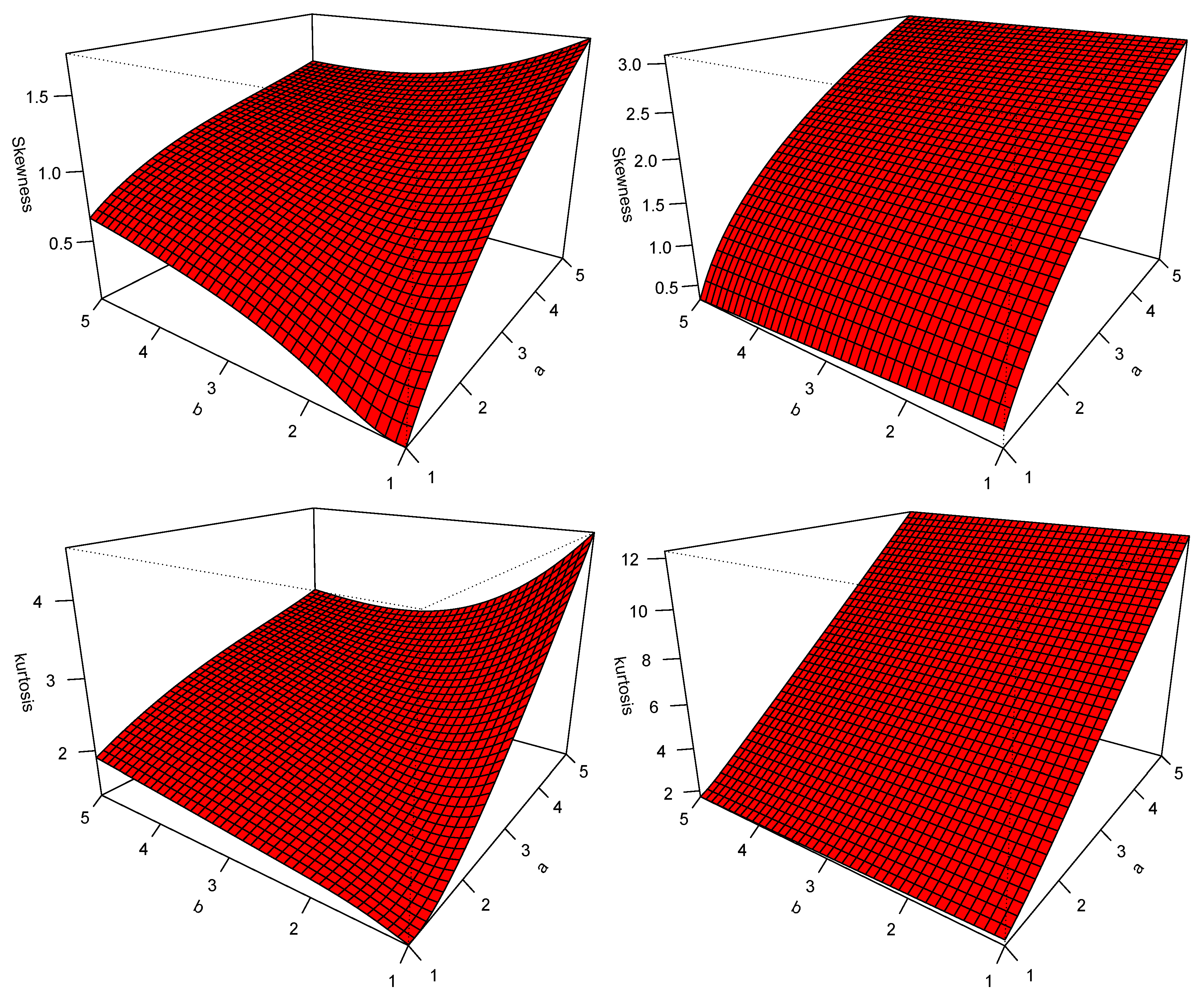
4.3. Mathematical Properties

Here we reported some mathematical properties of NKw-G family by using Equation (14) and those of the properties of the exp-G distribution.

Let $Y_{k,s}$ be a rv relating to exp-G model having power parameter $(k+s)$, then the rth ordinary moment of X, say $\mathbb{E}\left(X^r\right)$, can be expressed from Equation (14) as

$$\mathbb{E}\left(X^r\right)=\sum _{k=0}^{\infty }\sum _{s=0}^j{\omega }_{k,s}\mathbb{E}\left(Y_{k,s}^r\right)=\sum _{k=0}^{\infty }\sum _{s=0}^j{\omega }_{k,s}(k+s){\tau }_{r,k,s},$$

(15)

where ${\tau }_{r,k,s}={\int }_{-\infty }^{\infty }{x}^{r}G{(x;\xi )}^{k+s-1}g(x;\xi )dx={\int }_0^1{Q}_G{(u;\xi )}^r{u}^{k+s}du$, and $Q_G(u;\xi )$ is the qf of the baseline G.

The rth lower incomplete moment of X, say $m_r\left(y\right)={\int }_{-\infty }^y{x}^{r}f\left(x\right)dx$, is

$$\begin{array}{ccc}\hfill m_r\left(y\right)& =& \sum _{k=0}^{\infty }\sum _{s=0}^j{\omega }_{k,s}{\int }_{-\infty }^y{x}^r{h}_{k,s}\left(x\right)dx\hfill \\ & =& \sum _{k=0}^{\infty }\sum _{s=0}^j{\omega }_{k,s}{\int }_0^{G(y;\xi ))}{Q}_G{(u;\xi )}^r{u}^{k+s}du.\hfill \end{array}$$

(16)

The last two integrals can easily be evaluated numerically for most of the baseline G models.

The moment generating function (mgf)  $M\left(t\right)=\mathbb{E}\left({\mathrm{e}}^{tX}\right)$ of X follows from Equation (14) is

$$M\left(t\right)=\sum _{k=0}^{\infty }\sum _{s=0}^j{\omega }_{k,s}{M}_{k,s}\left(t\right)=\sum _{k=0}^{\infty }\sum _{s=0}^j{\omega }_{k,s}(k+s){\rho }_{k,s}\left(t\right),$$

(17)

where $M_{k,s}\left(t\right)$ is the mgf of $Y_{k,s}$ and ${\rho }_{k,s}\left(t\right)={\int }_0^{1}exp\left[t{Q}_G(u;\xi )\right]u^{k+s}du$. Hence, we can obtain the mgfs of many special NKw-G distributions directly from exp-G generating function and Equation (17).

The mode of NKw-G distribution is obtained by taking log of Equation (8) by

$$\begin{array}{ccc}\hfill log{f}_x(x;\xi )& =& log\left(ab\right)+log\left[g(x;\xi )\right]+G(x;\xi )+(a-1)log[1-(1-G(x;\xi ))exp\left[G(x;\xi )\right]]\hfill \\ & & +log\left[G(x;\xi )\right]+(b-1)log\left\{1-{[1-(1-G(x;\xi ))exp\left[G(x;\xi )\right]]}^a\right\}.\hfill \end{array}$$

(18)

Taking derivative with respect to x, the mode of NKw-G satisfies

$$\begin{array}{ccc}\hfill \frac{g^{\prime }(x;\xi )}{g(x;\xi )}+\frac{g(x;\xi )\left[\frac{aexp\left[G(x;\xi )\right]G(x;\xi )\left\{1-b{[1-(1-G(x;\xi ))exp\left[G(x;\xi )\right]]}^a\right\}}{1-{[1-(1-G(x;\xi ))exp\left[G(x;\xi )\right]]}^a}+\frac{1-e^{G(x;\xi )}}{G(x;\xi )}+1\right]}{1-(1-G(x;\xi \left)\right)exp\left[G\right(x;\xi \left)\right]}& =& 0.\hfill \end{array}$$

4.4. Estimation of Univariate G-Family Parameters

Here, we discuss the maximum likelihood estimation of NKw-G family parameters based on random samples $X_1,\dots ,X_n$ taken from any G distribution. The log-likelihood function $\ell (.)$ for vector $\mathbf{\theta }={(a,b,\xi )}^{\top }$ is

$$\begin{array}{ccc}\hfill \ell \left(\mathbf{\theta }\right)& =& nlog\left(ab\right)+\sum _{i=1}^{n}logg(x_i;\xi )+\sum _{i=1}^{n}logG(x_i;\xi )+(a-1)\sum _{i=1}^{n}log\left\{1-\overline{G}(x_i;\xi )exp\left[G(x_i;\xi )\right]\right\}\hfill \\ & & +\sum _{i=1}^{n}G(x_i;\xi )+(b-1)\sum _{i=1}^{n}log\left[1-{\left\{1-\overline{G}(x_i;\xi )exp\left[G(x_i;\xi )\right]\right\}}^a\right].\hfill \end{array}$$

The MLEs $\widehat{\mathbf{\theta }}$ of $\mathbf{\theta }$ can be evaluated by maximizing $\ell \left(\mathbf{\theta }\right)$. There exists several routines in literature which can be used for numerical maximization of $\ell \left(\mathbf{\theta }\right)$ particulary in R-language (optim function) and in Ox the (sub-routine MaxBFGS).

The score components obtained after differentiating the log-likelihood with respect to a, b and $\xi$ are:

$$\begin{array}{ccc}\hfill \frac{\partial \ell }{\partial a}& =& \frac{n}{a}-(b-1)\sum _{i=1}^n\frac{{\left\{1-\overline{G}(x_i;\xi )exp\left[G(x_i;\xi )\right]\right\}}^{a}log\left\{1-\overline{G}(x_i;\xi )exp\left[G(x_i;\xi )\right]\right\}}{1-{\left\{1-\overline{G}(x_i;\xi )exp\left[G(x_i;\xi )\right]\right\}}^a}\hfill \\ & & +\sum _{i=1}^{n}log\left\{1-\overline{G}(x_i;\xi )exp\left[G(x_i;\xi )\right]\right\},\hfill \\ \hfill \frac{\partial \ell }{\partial b}& =& \frac{n}{b}+\sum _{i=1}^{n}log\left[1-{\left\{1-\overline{G}(x_i;\xi )exp\left[G(x_i;\xi )\right]\right\}}^a\right],\hfill \\ \hfill \frac{\partial \ell }{\partial \xi }& =& \sum _{i=1}^n\frac{g_i^{\xi }}{g(x_i;\xi )}-\sum _{i=1}^n{G}_i^{\xi }+\sum _{i=1}^n\frac{G_i^{\xi }}{G(x_i;\xi )}+(a-1)\sum _{i=1}^n\frac{G(x_i;\xi )exp\left[G(x_i;\xi )\right]G_i^{\xi }}{1-\overline{G}(x;\xi )exp\left[G(x_i;\xi )\right]}\hfill \\ & & -(b-1)\sum _{i=1}^n\frac{aG(x_i;\xi )exp\left[G(x_i;\xi )\right]G_i^{\xi }{\left\{1-\overline{G}(x_i;\xi )exp\left[G(x_i;\xi )\right]\right\}}^{a-1}}{1-{\left\{1-\overline{G}(x_i;\xi )exp\left[G(x_i;\xi )\right]\right\}}^a},\hfill \end{array}$$

where $g_i^{\xi }=\frac{\partial }{\partial \xi }g(x_i;\xi )$ and $G_i^{\xi }=\frac{\partial }{\partial \xi }G(x_i;\xi )$ are derivatives of column vectors of the same dimension of $\xi$.

The MLEs of the model parameters can be obtained from the above score components after equating to zero, and then solving them simultaneously. If analytical solution is impossible, then analytical results for these parameters can be obtained through iterative algorithms.

For interval estimation of the parameters, we require the $3\times 3$ observed information matrix $I\left(\mathsf{\Theta }\right)=\{-I_{qs}\}$ (for $q,s=a,b,\xi$). Standard maximization routines provide only an approximation for the observed information matrix. The observed information matrix for the parameter vector $\mathsf{\Theta }={(a,b,\xi )}^{\top }$ is given by

$$I\left(\mathsf{\Theta }\right)=-\frac{{\partial }^2\ell \left(\mathsf{\Theta }\right)}{\partial \mathsf{\Theta }\partial {\mathsf{\Theta }}^{\top }}=-\left(\begin{array}{ccc}{I}_{aa}& I_{ab}& I_{a\xi }\\ \cdot & I_{bb}& I_{b\xi }\\ \cdot & \cdot & I_{\xi \xi }\end{array}\right).$$

Under standard regularity conditions, the multivariate normal $N_3(0,I{\left(\widehat{\mathsf{\Theta }}\right)}^{-1})$ distribution can be used to construct approximate confidence intervals for the model parameters. Here, $I(\widehat{\mathsf{\Theta }})$ is the total observed information matrix evaluated at $\widehat{\mathsf{\Theta }}$. Then, the $100(1-\sigma )\%$ confidence intervals for a, b and $\xi$ are given by $\widehat{a}\pm z_{{\sigma }^{*}/2}\times \sqrt{var\left(\widehat{a}\right)}$, $\widehat{b}\pm z_{{\sigma }^{*}/2}\times \sqrt{var(\widehat{b})}$ and $\widehat{\xi }\pm z_{{\sigma }^{*}/2}\times \sqrt{var(\widehat{\xi })}$, respectively, where the $var(·)$’s denote the diagonal elements of $I{(\widehat{\mathsf{\Theta }})}^{-1}$ corresponding to the model parameters, and $z_{{\sigma }^{*}/2}$ is the quantile ($1-{\sigma }^{*}/2$) of the standard normal distribution.

The standard errors of the estimated parameters are obtained by the inverse of $I\left(\mathsf{\Theta }\right)$.

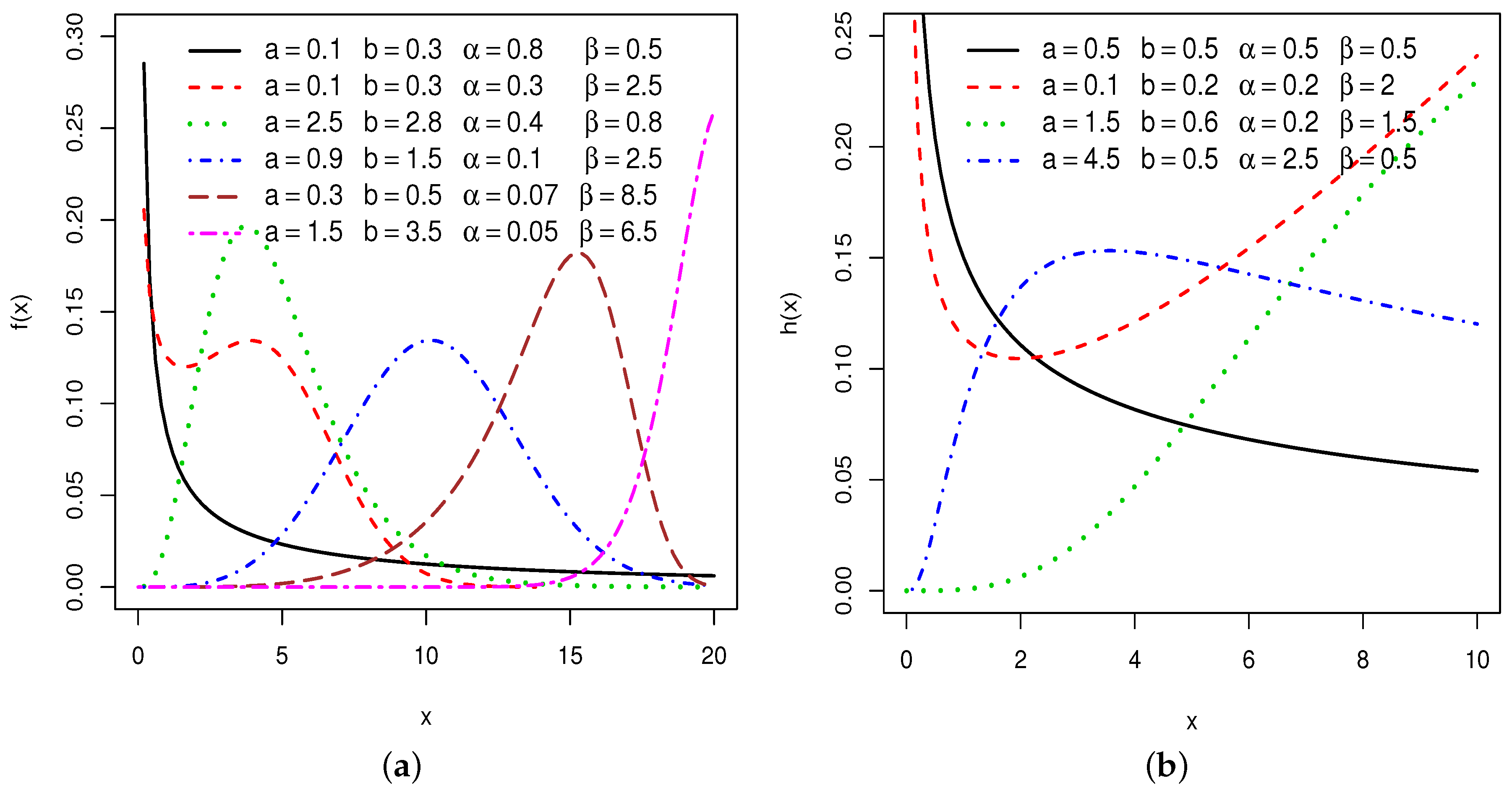
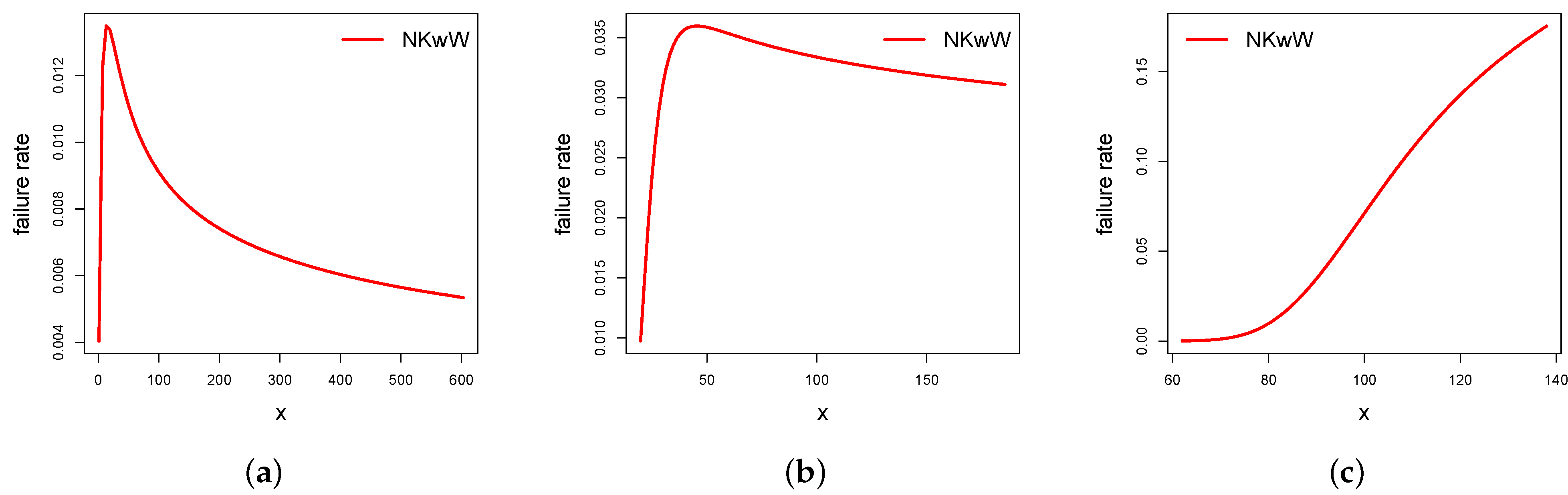
5. The Univariate NKwW Distribution

We now define the NKwW distribution by taking the Weibull baseline with cdf $G\left(x\right)=1-{\mathrm{e}}^{-{\left(\alpha x\right)}^{\beta }}$ and pdf $g\left(x\right)={\alpha }^{\beta }\beta x^{\beta -1}exp[-{\left(\alpha x\right)}^{\beta }]$. Then, the cdf and pdf of the NKwW distribution are, respectively, given by

$$\begin{array}{ccc}\hfill F_{NKwW}\left(x\right)& =& 1-{\left[1-{\left\{1-exp[-{\left(\alpha x\right)}^{\beta }]{\mathrm{e}}^{1-exp[-{\left(\alpha x\right)}^{\beta }]}\right\}}^a\right]}^b,x>0\hfill \end{array}$$

(19)

and

$$\begin{array}{ccc}\hfill f_{NKwW}\left(x\right)& =& ab{\alpha }^{\beta }\beta x^{\beta -1}exp[-{\left(\alpha x\right)}^{\beta }]{\mathrm{e}}^{1-exp[-{\left(\alpha x\right)}^{\beta }]}{\left\{1-exp[-{\left(\alpha x\right)}^{\beta }]{\mathrm{e}}^{1-exp[-{\left(\alpha x\right)}^{\beta }]}\right\}}^{a-1}\hfill \\ & \times & \left\{1-exp[-{\left(\alpha x\right)}^{\beta }]\right\}{\left[1-{\left\{1-exp[-{\left(\alpha x\right)}^{\beta }]{\mathrm{e}}^{1-exp[-{\left(\alpha x\right)}^{\beta }]}\right\}}^a\right]}^{b-1},x>0,\hfill \end{array}$$

(20)

where $\alpha >0$ is scale parameter and $\beta >0$ is shape parameter.

Henceforth, a random variable having density in Equation (20) is denoted by $X\sim \mathrm{NKwW}(a,b,\alpha ,\beta )$. The sf and hrf of X are given by

$$\begin{array}{ccc}\hfill S\left(x\right)& =& {\left[1-{\left\{1-exp[-{\left(\alpha x\right)}^{\beta }]{\mathrm{e}}^{1-exp[-{\left(\alpha x\right)}^{\beta }]}\right\}}^a\right]}^b,x>0\hfill \end{array}$$

and

$$\begin{array}{ccc}\hfill h\left(x\right)& =& ab{\alpha }^{\beta }\beta x^{\beta -1}exp[-{\left(\alpha x\right)}^{\beta }]{\mathrm{e}}^{1-exp[-{\left(\alpha x\right)}^{\beta }]}{\left\{1-exp[-{\left(\alpha x\right)}^{\beta }]{\mathrm{e}}^{1-exp[-{\left(\alpha x\right)}^{\beta }]}\right\}}^{a-1}\hfill \\ & & \times \left\{1-exp[-{\left(\alpha x\right)}^{\beta }]\right\}{\left[1-{\left\{1-exp[-{\left(\alpha x\right)}^{\beta }]{\mathrm{e}}^{1-exp[-{\left(\alpha x\right)}^{\beta }]}\right\}}^a\right]}^{-1},x>0.\hfill \end{array}$$

In Figure 1a,b, we display some plots of the density function and hrf of NKwW model for selected parameter values. From Figure 1a, it can be observed that NKwW density exhibits shapes such as unimodal (right-skewed, left skewed, symmetrical), J and reversed-J. From Figure 1b, one can depict that NKwW hazard rate shapes could be monotonic (increasing and decreasing) and non-monotonic (bathtub and upside-down bathtub).

5.1. Properties of Univariate NKwW Model

First, we will deduce linear representation of NKwW density to obtain useful properties of that model.

Following Equation (14), the NKwW density will become

$$f_{NKwW}\left(x\right)=\sum _{k=0}^{\infty }\sum _{s=0}^j{\omega }_{k,s}(k+s){\alpha }^{\beta }\beta x^{\beta -1}exp\{-{\left(\alpha x\right)}^{\beta }\}{\left[1-exp\{-{\left(\alpha x\right)}^{\beta }\}\right]}^{k+s-1},$$

(21)

is the density of exp-Weibull $(k+s,\alpha ,\beta )$, which after using generalized binomial expansion becomes

$$f_{NKwW}\left(x\right)=\sum _{p=0}^{k+s-1}{t}_p\pi (x;\alpha ,\beta ),$$

(22)

where $t_p={(-1)}^p\left(\genfrac{}{}{0pt}{}{k+s-1}{p}\right){\sum }_{k=0}^{\infty }{\sum }_{s=0}^j{\omega }_{k,s}(k+s)$ and $\pi (x;\alpha ,\beta )$ is the Weibull density.

From Equation (22) it is evident that NKwW density is actually a linear combination of Weibull densities. Therefore, several mathematical properties of NKwW model can easily be obtained from the properties of Weibull model.

Let $Z_p$ follows a density $\pi (x,\alpha ,\beta )$, then some properties of X can obtained from the properties of $Z_p$.

The expression for the qf of the NKwW distribution cannot be obtained explicitly. However, we can define it in term of Lambert-W function as

$$\begin{array}{cc}\hfill Q\left(u\right)=& \frac{1}{\alpha }{\left[1-log\left\{1-{\left[1-{(1-u)}^{1/b}\right]}^{1/a}\right\}+W\left\{\frac{{\left[1-{(1-u)}^{1/b}\right]}^{1/a}-1}{e}\right\}\right]}^{1/\beta }.\end{array}$$

(23)

For more detail about Lambert-W function, the reader is referred to Benkthehelifa [21].

The nth moment of X, say ${\mu }_r^{\prime }={\int }_0^{\infty }{x}^{r}f\left(x\right)dx$, is

$${\mu }_r^{\prime }=\sum _{p=0}^{k+s-1}{t}_p{\alpha }^{\beta }\beta {\int }_0^{\infty }{x}^r{x}^{\beta -1}exp\{-(p+1){\left(\alpha x\right)}^{\beta }\}dx.$$

(24)

After solving the last integral, the nth moment expression for X will be

$${\mu }_r^{\prime }=\Gamma \left(\frac{r}{\beta }+1\right)\sum _{p=0}^{k+s-1}\frac{t_p}{{\alpha }^r{(p+1)}^{r/\beta }}.$$

(25)

In general, some characteristics of a model can be obtained through moments especially mean, variance, skewness and kurtosis.

Table 1. First four moments of NKwW distribution for different parametric values.

a	b	$\mathit{\alpha }$	$\mathit{\beta }$	${\mathit{\mu }}_1^{\prime }$	${\mathit{\mu }}_2^{\prime }$	${\mathit{\mu }}_3^{\prime }$	${\mathit{\mu }}_4^{\prime }$
0.5	2.5	0.5	0.5	0.9387	4.3451	45.8866	863.8300
2.5	2.5	0.5	1.5	2.8303	8.5624	27.5141	93.4544
0.9	1.2	0.5	1.8	2.3023	6.1339	18.3379	60.3563
5.0	3.0	1.0	3.0	1.2997	1.7046	2.2555	3.0102

displays the first four moments of NKwW distribution on different parametric values using Equation (24). The skewness and kurtosis plots of NKwW model are displayed in Figure 2. These plots reveal that the parameters a and b play a significant role in modeling the skewness and kurtosis behaviors of X.

The rth incomplete moment expression can be written as

$$m_r\left(z\right)=\sum _{p=0}^{k+s-1}\frac{v_p}{{\alpha }^r{(p+1)}^{r/\beta }}\gamma \left(\frac{r}{\beta }+1,(p+1){\left(\alpha x\right)}^{\beta }\right),$$

(26)

where $\gamma (q,x)={\int }_0^{\infty }{x}^{q-1}exp(-x)dx$ is Euler gamma function.

5.2. Estimation of Univariate NKw Family Parameters

The log-likelihood function ℓ for the parameters vector $\mathbf{\theta }={(\alpha ,\beta ,a,b)}^{\top }$ of NKwW model given in Equation (20)

$$\begin{array}{ccc}\hfill \ell & =& nlog\left(ab{\alpha }^{\beta }\beta \right)+(\beta -1)\sum _{i=1}^{n}log\left(x_i\right)+\sum _{i=1}^{n}log\left\{1-exp[-{\left(\alpha x_i\right)}^{\beta }]\right\}-\sum _{i=1}^n{\left(\alpha x_i\right)}^{\beta }\hfill \\ & & +\sum _{i=1}^n\left\{1-exp[-{\left(\alpha x_i\right)}^{\beta }]\right\}+(a-1)\sum _{i=1}^{n}log\left\{1-exp[-{\left(\alpha x_i\right)}^{\beta }]{\mathrm{e}}^{1-exp[-{\left(\alpha x_i\right)}^{\beta }]}\right\}\hfill \\ & & +(b-1)\sum _{i=1}^{n}log\left[1-{\left\{1-exp[-{\left(\alpha x_i\right)}^{\beta }]{\mathrm{e}}^{1-exp[-{\left(\alpha x_i\right)}^{\beta }]}\right\}}^a\right].\hfill \end{array}$$

when maximizing the log-likelihood for constrained parameters, the parameters are often transformed to avoid the constraints and failure of Newton-Raphson [22]. This is the case of the proposed model since all the parameters are constrained (>0).

6. Simulation Study

Using Monte Carlo simulations, we now evaluate the asymptotic properties of the MLEs for the parameters of the NKwW model. The simulation study is repeated 1000 times with sample sizes of n = 50, 100, 200 and 500 with the following parameter scenarios: I: a = 0.9, b =1.5, $\alpha$ = 0.1, and $\beta$ = 2.5, II: a = 2.5, b =2.8, $\alpha$ = 0.4, and $\beta$ = 0.8, and III: a = 0.5, b =5.5, $\alpha$ = 1.5, and $\beta$ = 1.5. The random samples are generated using Equation (23).

Table 2. Average, Bias, MSE, SD, Average SE, CP, LB and UB for scenario-I.

		$\mathit{n}=50$				$\mathit{n}=100$
	a	b	$\mathit{\alpha }$	$\mathit{\beta }$	a	b	$\mathit{\alpha }$	$\mathit{\beta }$
Average	0.914	1.501	0.1	2.515	0.913	1.501	0.1	2.509
Bias	0.014	0.001	0.0	0.011	0.013	0.001	0.0	0.009
MSE	0.005	0.000	0.0	0.004	0.005	0.000	0.0	0.003
SD	0.103	0.031	0.006	0.067	0.067	0.014	0.003	0.046
Average SE	0.013	0.004	0.001	0.009	0.006	0.001	0.001	0.004
CP	0.928	0.886	1.000	0.997	0.921	0.879	1.000	0.995
LB	0.345	13.020	0.245	0.913	1.016	10.341	0.395	0.982
UB	1.350	15.544	0.576	2.905	2.301	12.286	0.792	3.353
		$\mathbf{n}=\mathbf{200}$				$\mathbf{n}=\mathbf{500}$
	a	b	$\mathbf{\alpha }$	$\mathbf{\beta }$	a	b	$\mathbf{\alpha }$	$\mathbf{\beta }$
Average	0.905	1.502	0.1	2.507	0.904	1.501	0.1	2.503
Bias	0.005	0.002	0.0	0.007	0.004	0.001	0.0	0.003
MSE	0.003	0.000	0.0	0.003	0.001	0.000	0.0	0.000
SD	0.062	0.023	0.003	0.061	0.028	0.008	0.002	0.024
Average SE	0.004	0.001	0.0001	0.004	0.001	0.0002	0.000	0.001
CP	0.93	0.910	1.000	0.99	0.947	0.988	1.000	0.982
LB	0.211	11.130	0.166	0.963	0.244	7.910	0.108	1.056
UB	0.983	14.164	0.452	2.585	0.795	11.150	0.366	2.205

,

Table 3. Average, Bias, MSE, SD, Average SE, CP, LB and UB for scenario-II.

		$\mathit{n}=50$				$\mathit{n}=100$
	a	b	$\mathit{\alpha }$	$\mathit{\beta }$	a	b	$\mathit{\alpha }$	$\mathit{\beta }$
Average	2.519	2.775	0.405	0.831	2.520	2.775	0.404	0.821
Bias	0.019	−0.025	0.005	0.031	0.020	−0.025	0.004	0.021
MSE	0.168	0.054	0.007	0.012	0.148	0.051	0.006	0.007
SD	0.424	0.240	0.088	0.109	0.344	0.199	0.070	0.081
Average SE	0.058	0.033	0.012	0.015	0.039	0.022	0.007	0.008
CP	0.883	0.868	0.998	0.961	0.873	0.855	1.000	0.949
LB	13.682	15.354	3.052	1.379	6.780	12.997	1.213	1.269
UB	19.074	17.775	4.216	3.868	11.046	15.678	2.096	3.521
		$\mathbf{n}=\mathbf{200}$				$\mathbf{n}=\mathbf{500}$
	a	b	$\mathbf{\alpha }$	$\mathbf{\beta }$	a	b	$\mathbf{\alpha }$	$\mathbf{\beta }$
Average	2.494	2.801	0.399	0.809	2.490	2.800	0.399	0.806
Bias	−0.006	0.002	−0.001	0.009	−0.006	0.001	−0.001	0.006
MSE	0.042	0.012	0.002	0.003	0.040	0.011	0.002	0.002
SD	0.218	0.117	0.044	0.053	0.217	0.112	0.042	0.041
Average SE	0.016	0.009	0.003	0.004	0.010	0.005	0.002	0.002
CP	0.866	0.870	0.988	0.940	0.848	0.899	0.998	0.879
LB	5.042	9.692	1.056	0.879	3.450	8.729	0.547	0.740
UB	9.145	12.739	1.839	2.921	7.240	12.422	1.122	2.520

and

Table 4. Average, Bias, MSE, SD, Average SE, CP, LB and UB for scenario-III.

		$\mathit{n}=50$				$\mathit{n}=100$
	a	b	$\mathit{\alpha }$	$\mathit{\beta }$	a	b	$\mathit{\alpha }$	$\mathit{\beta }$
Average	0.590	5.525	1.740	1.566	0.539	5.512	1.609	1.550
Bias	0.090	0.025	0.240	0.066	0.039	0.012	0.109	0.050
MSE	0.102	0.017	0.446	0.260	0.041	0.007	0.157	0.143
SD	0.282	0.111	0.575	0.474	0.192	0.077	0.362	0.364
Average SE	0.039	0.016	0.077	0.070	0.021	0.008	0.039	0.038
CP	0.998	0.849	1.000	0.998	0.997	0.851	1.000	1.000
LB	3.631	56.393	58.803	1.329	1.044	42.404	11.521	1.173
UB	5.319	60.696	73.584	3.463	2.259	46.958	22.151	3.020
		$\mathbf{n}=\mathbf{200}$				$\mathbf{n}=\mathbf{500}$
	a	b	$\mathbf{\alpha }$	$\mathbf{\beta }$	a	b	$\mathbf{\alpha }$	$\mathbf{\beta }$
Average	0.523	5.507	1.567	1.552	0.514	5.503	1.531	1.504
Bias	0.023	0.007	0.067	0.052	0.014	0.003	0.031	0.004
MSE	0.026	0.005	0.082	0.118	0.008	0.001	0.023	0.042
SD	0.148	0.071	0.256	0.337	0.086	0.032	0.142	0.199
Average SE	0.010	0.0043	0.017	0.023	0.004	0.001	0.006	0.009
CP	0.997	0.891	0.999	0.999	0.993	0.903	1.000	0.998
LB	0.556	35.430	7.104	1.033	0.340	25.285	4.695	1.009
UB	1.528	40.668	16.144	2.674	1.021	31.077	12.4051	2.271

display the average estimate (Average), average bias (Bias) of the MLEs, mean square error (MSE), average standard error (Average SE), standard deviation (SD), model-based coverage probabilities (CP), lower bound (LB) and upper bound (UB) for the parameters a, b, $\alpha$ and $\beta$, respectively, for these scenarios and sample sizes. We conclude from the simulation findings that MLEs perform well in estimating parameters a, b, $\alpha$ and $\beta$. The CPs of the confidence intervals are quite close to the 95% nominal levels. It is apparent that the bias and MSE decreases as the sample size increases. This gives an indication that maximum likelihood method has performed well while estimation of NKwW model parameters. The related bias, MSE, SD and Average SE are, respectively, defined by

$$Bias\left(\widehat{\mathbf{\theta }}\right)=\sum _{i=1}^N\frac{\widehat{{\mathbf{\theta }}_i}}{N}-\mathbf{\theta },MSE\left(\widehat{\mathbf{\theta }}\right)=\sum _{i=1}^N\frac{{(\widehat{{\mathbf{\theta }}_i}-\mathbf{\theta })}^2}{N},$$

$$SD\left(\widehat{\mathbf{\theta }}\right)=\sqrt{\frac{{\sum }_{i=1}^N{\left(\widehat{{\mathbf{\theta }}_i}-\mathbf{\theta }\right)}^2}{N-1}}\mathrm{and}AverageSE\left(\widehat{\mathbf{\theta }}\right)=\frac{SD}{\sqrt{N}}=\sqrt{\frac{N}{N-1}}\sqrt{{\sum }_{i=1}^N{\left(\widehat{{\mathbf{\theta }}_i}-\mathbf{\theta }\right)}^2}.$$

For the 95% confidence intervals of the MLEs, we calculate the empirical coverage probability (CP) which is defined by

$$CP\left(\widehat{\mathbf{\theta }}\right)=\frac{1}{N}\sum _{i=1}^{N}I\left(\widehat{{\theta }_i}-1.9599s_{\widehat{{\theta }_i}}<\mathbf{\theta }<\widehat{{\theta }_i}+1.9599s_{\widehat{{\theta }_i}}\right),$$

where $I(.)$ is the indicator function and $s_{\widehat{{\mathbf{\theta }}_i}}=\left(s_{\widehat{{\alpha }_i}},s_{\widehat{{\beta }_i}},s_{\widehat{a_i}},s_{\widehat{b_i}}\right)$ are the standard errors of the MLEs.

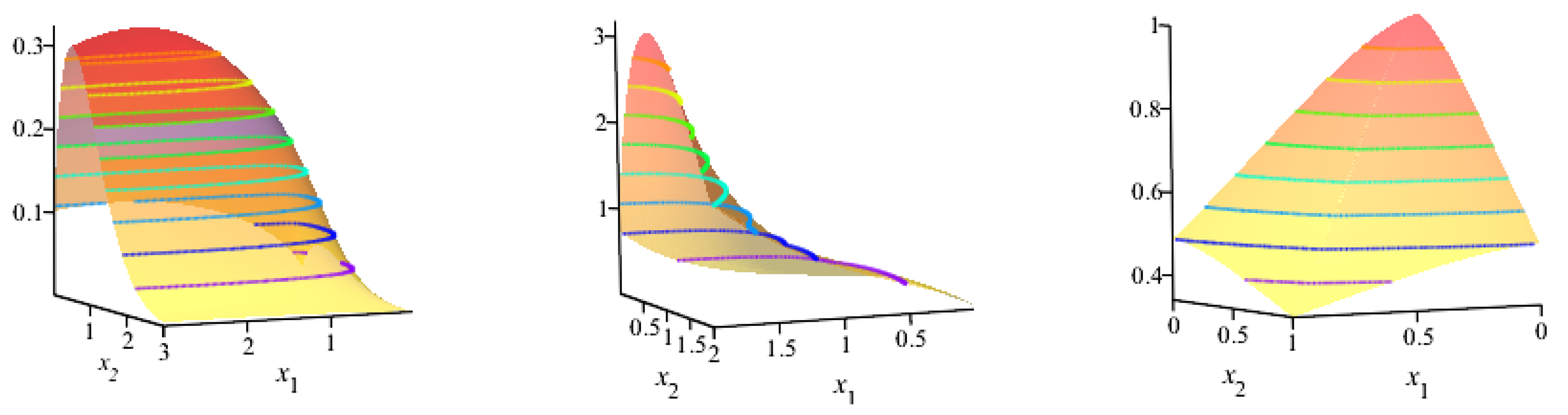
7. Bivariate New Kumaraswamy (BvNKw) G-Family

In this Section, we introduce a bivariate extension of the NKw-G univariate family by considering Marshall and Olkin shock model (see, Marshall and Olkin [23]). This approach has been adopted by Kundu and Gupta [24], Barreto-Souza and Lemonte [25], Ghosh and Hamedani [26], Eliwa and El-Morshedy [27], El-Morshedy et al. [28,29] etc. among others, for developing bivariate extensions of the well-known parent models. The BvNKw-G family is constructed from three independent NKw-G families using a minimization process. Assuming that the three independent rvs are $Z_1\sim \mathrm{NKw}-\mathrm{G}(b_1,a,\xi )$, $Z_2\sim \mathrm{NKw}-\mathrm{G}(b_2,a,\xi )$ and $Z_3\sim \mathrm{NKw}-\mathrm{G}(b_3,a,\xi )$. Define $X_1=min\{Z_1,Z_3\}$ and $X_2=min\{Z_2,Z_3\}$. Thus, the random vector $X=(X_1,X_2)$ is said to have the BvNKw-G family with parameters vector $\mathsf{\Omega }=(b_1,b_2,b_3,a,\xi$) if its joint reliability function (jrf) is given by

$${\overline{F}}_{X_1,X_2}(x_1,x_2)=\left\{\begin{array}{c}{S}_{\mathrm{NKw}-\mathrm{G}}(x_1;b_1,a,\xi )S_{\mathrm{NKw}-\mathrm{G}}(x_2;b_2+b_3,a,\xi )\mathrm{if}{x}_1\le x_2,\hfill \\ S_{\mathrm{NKw}-\mathrm{G}}(x_1;b_1+b_3,a,\xi )S_{\mathrm{NKw}-\mathrm{G}}(x_2;b_2,a,\xi )\mathrm{if}{x}_1>x_2.\hfill \end{array}\right.$$

(27)

The marginal rfs of the BvNKw-G family are

$${\overline{F}}_{X_i}\left(x_i\right)=Pr\left(min\{T_i,T_3\}>x_i\right)={\overline{F}}_{\mathrm{NKw}-\mathrm{G}}(x_i;b_i+b_3,a,\xi );i=1,2.$$

(28)

The joint pdf (jpdf) corresponding to Equation (27) is

$$f_{X_1,X_2}(x_1,x_2)=\left\{\begin{array}{c}{f}_{\mathrm{NKw}-\mathrm{G}}(x_1;b_1,a,\xi )f_{\mathrm{NKw}-\mathrm{G}}(x_2;b_2+b_3,a,\xi )\mathrm{if}0<x_1<x_2<\infty ,\hfill \\ f_{\mathrm{NKw}-\mathrm{G}}(x_1;b_1+b_3,a,\xi )f_{\mathrm{NKw}-\mathrm{G}}(x_2;b_2,a,\xi )\mathrm{if}0<x_2<x_1<\infty ,\hfill \\ \frac{b_3}{b_1+b_2+b_3}{f}_{\mathrm{NKw}-\mathrm{G}}(x;b_1+b_2+b_3,a,\xi )\mathrm{if}0<x_1=x_2=x<\infty .\hfill \end{array}\right.$$

(29)

The jpdf over the domains $0<x_1<x_2<\infty$ and $0<x_2<x_1<\infty$ can be obtained by differentiating Equation (27) with respect to $x_1$ and $x_2$, whereas the jpdf over the domain $0<x_1=x_2=x<\infty$ can be derived from a well-known formula (see Eliwa and El-Morshedy [27]). The marginal pdfs corresponding to Equation (28) can be proposed as

$$f_{X_i}\left(x_i\right)=f_{\mathrm{NKw}-\mathrm{G}}(x_i;b_i+b_3,a,\xi );i=1,2.$$

(30)

Using Equations (27) and (29), the joint hrf (jhrf) can easily be derived by using $h_{X_1,X_2}(x_1,x_2)=\frac{f_{X_1,X_2}(x_1,x_2)}{{\overline{F}}_{X_1,X_2}(x_1,x_2)}$. In Figure 3, Figure 4 and Figure 5, some plots of the jpdf, jhrf, and jrf are presented for selected values of the BvNKw-Weibull (BvNKwW) parameters.

If X have the BvNKw-G family, then the distributions of $max\{X_1,X_2\}$ and $min\{X_1,X_2\}$ are

$$F_{max\{X_1,X_2\}}\left(t\right)=\prod _{i=1}^3{F}_{NKw-G}(t;b_i,a,\xi )\mathrm{and}{F}_{min\{X_1,X_2\}}\left(t\right)=1-\prod _{i=1}^3{\overline{F}}_{NKw-G}(t;b_i,a,\xi ),$$

respectively. If $X_1\sim \mathrm{NKw}-G(b_1+b_3,a,\xi )$ and $X_2\sim \mathrm{NKw}-\mathrm{G}(b_2+b_3,a,\xi )$, then the qf for the marginals is

$$Q{\left(u\right)}_{X_i}=G^{-1}\left[W\left({\mathrm{e}}^{-1}{\left[1-{(1-u)}^{1/(b_i+b_3)}\right]}^{1/a}-1\right)+1\right];i=1,2.$$

(31)

Using (31), the coefficient of correlation between $X_1$ and $X_2$ is

$$Q{\left(u\right)}_{X_1,X_2}=\left\{\begin{array}{c}4F_{\mathrm{NKw}-\mathrm{G}}\left(Q{\left(u\right)}_{X_2};b_2+b_3,a,\xi \right)F_{\mathrm{NKw}-\mathrm{G}}\left(Q{\left(u\right)}_{X_1};b_1,a,\xi \right)-1\mathrm{if}{x}_1<x_2\hfill \\ 4F_{\mathrm{NKw}-\mathrm{G}}\left(Q{\left(u\right)}_{X_1};b_1+b_3,a,\xi \right)F_{\mathrm{NKw}-\mathrm{G}}\left(Q{\left(u\right)}_{X_2};b_2,a,\xi \right)-1\mathrm{if}{x}_1>x_2.\hfill \end{array}\right.$$

(32)

The coefficient of median correlation between $X_1$ and $X_2$ can be derived at $u=0.5$. The BvNKw-G family exhibits both characteristics such as absolute continuous as well as singular part likewise reported in Marshall and Olkin’s bivariate exponential model. Thus, the joint distribution function (jdf) of $X_1$ and $X_2$ exhibits a singular part along the line $x_1=x_2$ having weight $b_3/(b_1+b_2+b_3)$, and an absolute continuous part for $0<$$x_1\ne x_2$<∞ having weight $(b_1+b_2)/(b_1+b_2+b_3)$. If ${\gamma }_i={\overline{F}}_{X_i}\left(x_i\right)$ where $X_i\sim \mathrm{NKw}-\mathrm{G}(b_i+b_3,a,\xi );$$i=1,2$, then the jrf by utilizing the Marshall-Olkin copula will be as follows:

$${\overline{F}}_{X_1,X_2}(x_1,x_2)={\gamma }_1^{1-{\mathsf{\Omega }}_1}{\gamma }_2^{1-{\mathsf{\Omega }}_2}max\left({\gamma }_1^{{\mathsf{\Omega }}_1},{\gamma }_2^{{\mathsf{\Omega }}_2}\right),\mathrm{for}0<{\mathsf{\Omega }}_1,{\mathsf{\Omega }}_2<1,$$

where ${\mathsf{\Omega }}_i=\frac{b_3}{b_i+b_3}.$

7.1. The MLE for the BvNKw-G Parameters

Here we dealt with the estimation of BvNKw-G family parameters through maximum likelihood method. Suppose that $(x_{11},x_{21}),(x_{12},x_{22}),\dots ,(x_{1m},x_{2m})$ is a sample of size m from the BvNKw-G family where ${\mathsf{\Psi }}_1=\{x_{1i}<x_{2i}\}$, ${\mathsf{\Psi }}_2=\{x_{1i}>x_{2i}\}$, ${\mathsf{\Psi }}_3=\{x_{1i}=x_{2i}=x_i\}$, $\left|{\mathsf{\Psi }}_1\right|=m_1,$$\left|{\mathsf{\Psi }}_2\right|=m_2$, $\left|{\mathsf{\Psi }}_3\right|=m_3$ and $\left|\mathsf{\Psi }\right|={\sum }_{i=1}^3{m}_i=m$. Using Equation (29), the likelihood function $\ell \left(\mathsf{\Omega }\right)$ can be written as

$$\begin{array}{ccc}\hfill \ell \left(\mathsf{\Omega }\right)& =& \prod _{i=1}^{m_1}{f}_{\mathrm{NKw}-\mathrm{G}}(x_{1i};b_1,a,\xi )f_{\mathrm{NKw}-\mathrm{G}}(x_{2i};b_2+b_3,a,\xi )\prod _{i=1}^{m_2}{f}_{\mathrm{NKw}-\mathrm{G}}(x_{1i};b_1+b_3,a,\xi )\hfill \\ & & \times f_{\mathrm{NKw}-\mathrm{G}}(x_{2i};b_2,a,\xi )\prod _{i=1}^{m_3}\frac{b_3}{b_1+b_2+b_3}{f}_{\mathrm{NKw}-\mathrm{G}}(x_i;b_1+b_2+b_3,a,\xi ).\hfill \end{array}$$

(33)

Differentiating after taking logarithm of the above likelihood function with respect to parameters $b_1$, $b_2$, $b_3$, a and $\xi$, and then equating them equal to zero can help in obtaining estimates of the bivariate model. If the solution is not possible, then optimization methods can be adopted to obtain numerical results.

7.2. Kendall’s Rank Correlation ($\tau$)

Assume ($W_1,W_2$) and ($Z_1,Z_2$) are two independent and identically distributed random vectors, then the $\tau$ is defined as follows

$$\tau =P\left[\left(W_1-Z_1\right)\left(W_2-Z_2\right)>0\right]-P\left[\left(W_1-Z_1\right)\left(W_2-Z_2\right)<0\right].$$

(34)

Nelsen [30] has shown that the $\tau$ is also a copula property. The BvNKwW distribution can be obtained using the copula function also. For every bivariate distribution function, with continuous marginals $F_{X_1}\left(x_1\right)$ and $F_{X_2}\left(x_2\right)$, corresponds a unique function $C:{[0,1]}^2\to [0,1]$, called a copula such that

$$F_{X_1,X_2}(x_1,x_2)=C(F_{X_1}\left(x_1\right),F_{X_2}\left(x_2\right)),$$

where $C(.,.)$ is the Clayton copula (see Nelsen [30,31]). Thus, if $(Z_1,Z_2)$ has the BvNKwW family, the $\tau$ between $Z_1$ and $Z_2$ is given by

$$\tau ={\int }_0^1{\int }_0^{1}C(u,v)\frac{{\partial }^{2}C(u,v)}{\partial u\partial v}dudv-1.$$

(35)

7.3. Simulation for the BvNKw-G Family

In this section, the MLE method is used to estimate the parameters $b_1,b_2,b_3,\alpha ,\beta$ and a of the BvNKwW distribution. The population parameters are generated using software R package. The sampling distributions are obtained for different sample sizes $n=$ 50, 100, 200 from $N=$1000 replications. This study proposed an assessment of the properties of the MLE for the parameters.

Table 5. Simulation results for the BvNKwW model.

	$n=50$
	${\mathit{b}}_{\mathbf{1}}$	${\mathit{b}}_{\mathbf{2}}$	${\mathit{b}}_{\mathbf{3}}$	$\mathbf{\alpha }$	$\mathbf{\beta }$	$\mathit{a}$
Average	3.254	3.325	3.145	0.485	1.536	0.334
Bias	0.014	0.034	0.029	−0.015	0.085	0.074
MSE	0.024	0.037	0.019	0.018	0.035	0.085
SD	0.021	0.031	0.014	0.012	0.027	0.079
CP	0.857	0.967	0.898	0.923	0.991	0.935
LB	2.987	2.854	2.334	0.259	1.183	0.227
UP	4.117	4.598	4.969	0.743	1.887	0.633
	$\mathit{n}=\mathbf{100}$
	${\mathit{b}}_{\mathbf{1}}$	${\mathit{b}}_{\mathbf{2}}$	${\mathit{b}}_{\mathbf{3}}$	$\mathit{\alpha }$	$\mathit{\beta }$	$\mathit{a}$
Average	3.165	3.214	3.098	0.489	1.523	0.321
Bias	0.008	0.023	0.015	−0.011	0.049	0.036
MSE	0.008	0.017	0.012	0.012	0.024	0.056
SD	0.004	0.012	0.007	0.003	0.017	0.044
CP	0.998	0.876	0.964	0.876	0.910	0.962
LB	2.597	2.367	2.122	0.377	1.101	0.245
UP	3.911	3.637	3.876	0.864	2.018	0.886
	$\mathit{n}=\mathbf{200}$
	${\mathit{b}}_{\mathbf{1}}$	${\mathit{b}}_{\mathbf{2}}$	${\mathit{b}}_{\mathbf{3}}$	$\mathit{\alpha }$	$\mathit{\beta }$	$\mathit{a}$
Average	3.072	3.110	3.025	0.496	1.513	0.313
Bias	0.003	0.007	0.008	−0.007	0.013	0.022
MSE	0.006	0.009	0.008	0.007	0.014	0.037
SD	0.001	0.004	0.002	0.001	0.007	0.024
CP	0.931	0.894	0.910	0.883	0.905	0.899
LB	2.157	2.367	2.110	0.159	1.017	0.119
UP	4.336	4.980	4.730	0.969	2.340	0.887

reports the simulation results for the BvNKwW model for $b_1=3$, $b_2=3$, $b_3=3$, $\alpha =0.5$, $a=0.3$, $\beta =1.5$ with different sample sizes.

From Table 5, it is observed that the bias and MSE are reduced as the sample size is increased for the MLE. Further, the results of simulation indicate that the BvNKwW distribution works well under the situation where no censoring occurs.

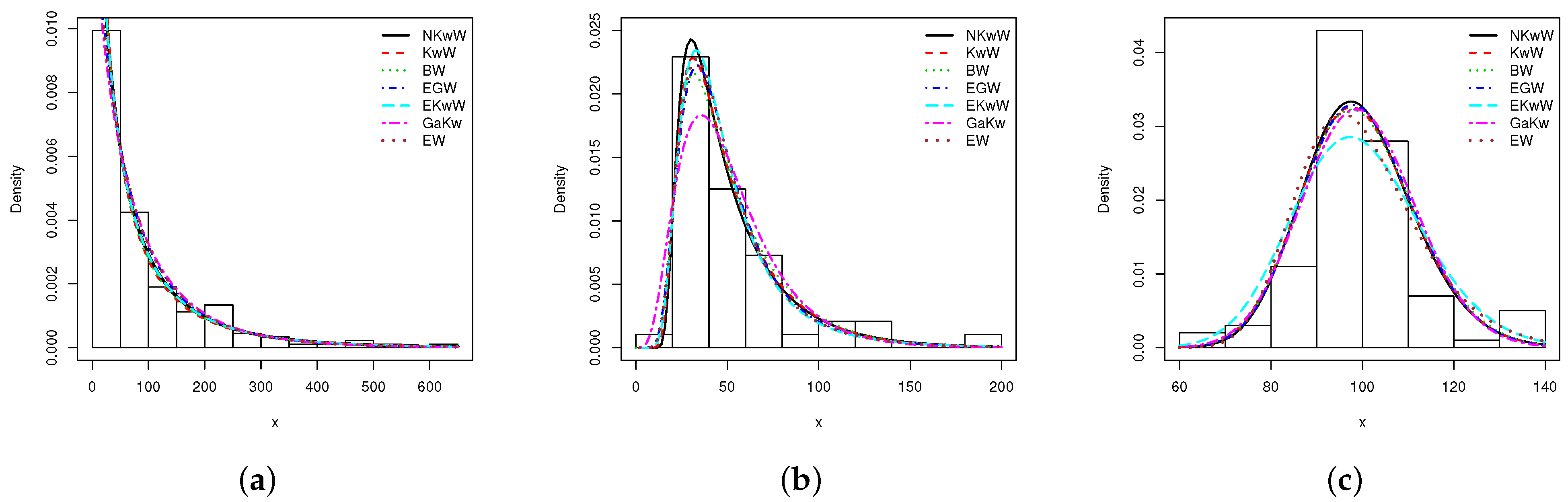
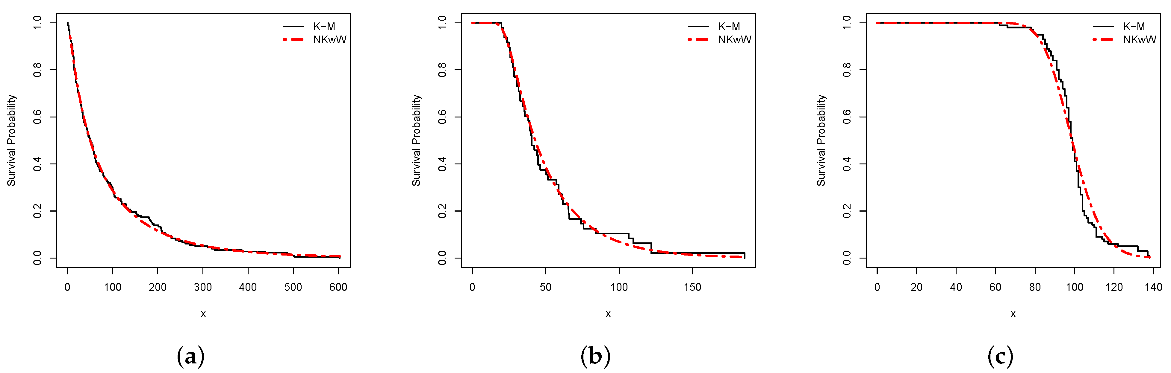
8. Empirical Illustrations of the Proposed Univariate Model

We compare the newly proposed 4-parameter model, NKwW distribution, with some well-established models viz. 4-parameter Kumaraswamy-Weibull [32], 4-parameter beta-Weibull [33], 4-parameter exponentiated-generalized Weibull [34], 5-parameter exponentiated Kumaraswamy-Weibull [35], 3-parameter gamma-Weibull [36], 3-parameter exponentiated-Weibull [37] and 2-parameter Weibull [38] distributions.

Table 6. Some well-established competitive models.

Some Well—Established Models	Abbrivations
Kumaraswamy-Weibull	KwW
Beta-Weibull	BW
Exponentiated-generalized Weibull	EGW
Exponentiated Kumaraswamy-Weibull	EKwW
Gamma-Weibull	GaW
Exponentiated-Weibull	EW
Weibull	W

shows the abbreviation of some well–established competitive models.

Three real-life data sets, namely, Air Conditioned Failures Data [39], Flood Data [40] and Breaking Strength Data [41] (see Appendix A for data sets) are used to compare and illustrate the potentiality of NKwW model.

The MLEs ($\widehat{\ell }$) and the standard errors (SEs) of the estimates, and the results of goodness-of-fit (GoF) criterion viz. Akaike information criterion (AIC), Bayesian Information Criterion (BIC), Hannan-Quinn Information Criterion (HQIC), Anderson-Darling (AD), Cramér–von Mises (CvM) and Kolmogrov-Smirnov (KS) are computed using AdequacyModel package in R-Statistical Computing Environment written by Marinho et al. [42]. Then, GoF values of all models are compared to search for the best model. The lower values of GoF statistics (GoFS) and high KS p-values indicate good fits.

In

Table 7. The MLEs and their SEs (in parentheses) of all competing models for Air Conditioned Failures Data set.

Model	a	b	$\mathit{\alpha }$	$\mathit{\beta }$	$\mathit{\theta }$
NKwW	1.4234	0.1476	0.1570	0.7035	-
	(0.3004)	(0.0123)	(0.0093)	(0.0059)	-
KwW	6.9878	0.1371	0.4437	0.6404
	(0.0674)	(0.0104)	(0.0033)	(0.0026)	-
BW	3.8696	0.1436	0.3662	0.6566	-
	(0.7402)	(0.0124)	(0.0047)	(0.0063)	-
EGW	1.3659	1.6063	0.0128	0.7089	-
	(0.8344)	(0.4839)	(0.0103)	(0.1106)	-
EKwW	3.5743	0.1525	0.1756	0.7516	0.8511
	(0.1978)	(0.0192)	(0.0165)	(0.0110)	(0.0888)
GaW	1.2854	-	0.0174	0.7854	-
	(0.3523)	-	(0.0082)	(0.1273)	-
EW	1.5398	-	0.0188	0.7278	-
	(0.4638)	-	(0.0068)	(0.1143)	-
W	-	-	0.0118	0.9057	-
	-	-	(0.0010)	(0.0512)	-

,

Table 8. The MLEs and their standard errors (in parentheses) for Flood Data set.

Model	a	b	$\mathit{\alpha }$	$\mathit{\beta }$	$\mathit{\theta }$
NKwW	47.4853	0.2245	0.2413	0.8860	-
	(1.2203)	(0.0747)	(0.0365)	(0.0898)	-
KwW	54.7825	0.2041	0.1609	1.0252	-
	(0.1358)	(0.0382)	(0.0153)	(0.0276)	-
BW	23.0602	0.1940	0.1320	1.1080	-
	(8.7941)	(0.0324)	(0.0073)	(0.0068)	-
EGW	5.5966	10.5493	0.0090	0.7774	-
	(2.0458)	(5.6821)	(0.0041)	(0.1370)	-
EKwW	13.5103	0.2625	1.0662	0.6682	10.4554
	(1.4869)	(0.0374)	(0.0114)	(0.0093)	(3.4956)
GaW	14.7225	-	4.6144	0.4983	-
	(1.7239)	-	(0.1518)	(0.0217)	-
EW	113.6840	-	0.7698	0.4651	-
	(142.9147)	-	(1.0663)	(0.1165)	-
W	-	-	0.0171	1.7719	-
	-	-	(0.0015)	(0.1776)	-

and

Table 9. The MLEs and their SEs (in parentheses) of all competing models for Breaking Strength Data set.

Model	a	b	$\mathit{\alpha }$	$\mathit{\beta }$	$\mathit{\theta }$
NKwW	10.3003	1.9955	0.0179	2.0187	-
	(5.5072)	(0.9568)	(0.0029)	(0.3505)	-
KwW	12.3850	1.4312	0.0143	2.7814	-
	(6.5412)	(0.8195)	(0.0018)	(0.6625)	-
BW	6.8561	0.6098	0.0133	4.1015	-
	(4.8522)	(0.3226)	(0.0016)	(1.0461)	-
EGW	0.4074	8.6459	0.0171	3.5077	-
	(0.2631)	(5.8742)	(0.0037)	(0.7875)	-
EKwW	1.1559	3.1680	0.0096	3.0390	6.7019
	(0.2743)	(1.4522)	(0.0013)	(0.4169)	(2.1035)
GaW	14.4806	-	0.0353	2.1128	-
	(2.5218)	-	(0.0050)	(0.1240)	-
EW	42.8741	-	0.0199	2.1092	-
	(21.3162)	-	(0.0026)	(0.2529)	-
W	-	-	0.0095	7.5137	-
	-	-	(0.0001)	( 0.5450)	-

, the values of MLEs and their SEs are listed for the NKwW, KwW, BW, EGW, EKwW, GaW, EW and W models, when applied to three real-life data sets. In

Table 10. The values of GoFS AIC, BIC, HQIC, AD, CvM, KS and KS p-value of all competing models for Air Conditioned Failures Data set.

								KS
Model	$-\widehat{\mathit{\ell }}$	AIC	BIC	HQIC	AD	CvM	KS	p-Value
NKwW	976.7081	1961.4160	1974.1660	1966.5860	0.1954	0.0238	0.0377	0.9615
KwW	978.2675	1964.5350	1977.2850	1969.7050	0.2925	0.0313	0.0388	0.9501
BW	977.0803	1962.1610	1974.9100	1967.3300	0.2001	0.0219	0.0391	0.9470
EGW	978.7362	1965.4720	1978.2220	1970.6420	0.5620	0.0878	0.0420	0.9100
EKwW	977.6941	1963.3880	1979.3250	1969.8510	0.1918	0.0229	0.0388	0.9505
GaW	979.8445	1965.6890	1975.2510	1969.5660	0.7633	0.1219	0.0504	0.7530
EW	978.8859	1963.7720	1974.3340	1967.6490	0.5957	0.0935	0.0440	0.8797
W	981.1477	1966.2950	1975.6700	1968.8800	0.9755	0.1577	0.0567	0.6123

,

Table 11. The values of GoFS AIC, BIC, HQIC, AD, CvM, KS and KS p-value of all competing models for Flood Data set.

								KS
Model	$-\widehat{\mathit{\ell }}$	AIC	BIC	HQIC	AD	CvM	KS	p-Value
NKwW	215.0072	438.0144	445.4992	440.8429	0.1725	0.0235	0.0691	0.9761
KwW	215.5195	439.0389	446.5238	441.8675	0.2495	0.0347	0.0834	0.8924
BW	216.1573	440.3147	447.7995	443.1432	0.3387	0.0477	0.0973	0.7538
EGW	218.1801	444.3601	451.8449	447.1887	0.6147	0.0913	0.0973	0.7543
EKwW	216.8837	443.7674	453.1234	447.3031	0.4183	0.0609	0.0893	0.8387
GaW	219.4700	444.9401	450.5537	447.0615	0.8278	0.1250	0.1176	0.5203
EW	216.1707	438.7413	445.9549	440.4627	0.3006	0.0430	0.0763	0.9428
W	225.7065	455.4131	459.1555	456.8273	1.7286	0.2765	0.1399	0.3048

and

Table 12. The values of GoFS AIC, BIC, HQIC, AD, CvM, KS and KS p-value of all competing models for Breaking Strength Data set.

								KS
Model	$-\widehat{\mathit{\ell }}$	AIC	BIC	HQIC	AD	CvM	KS	p-Value
NKwW	391.4242	790.8485	801.2692	795.0659	2.1765	0.3684	0.1349	0.0525
KwW	391.6541	791.3081	801.7288	795.5256	2.2478	0.3781	0.1372	0.0463
BW	392.1492	792.2985	802.7192	796.5159	2.3690	0.3983	0.1446	0.0305
EGW	391.8419	791.6838	802.1045	795.9012	2.3105	0.3878	0.1417	0.0361
EKwW	393.8688	797.7376	810.7635	803.0094	2.3206	0.3892	0.1544	0.0170
GaW	393.0037	792.0073	799.8228	795.1704	2.5727	0.4276	0.1511	0.0208
EW	393.8216	793.6431	801.6586	796.8062	2.4039	0.4211	0.1363	0.0505
W	404.7118	813.4235	818.6339	815.5323	4.7488	0.7985	0.1978	0.0008

, the numerical values of the GoFS are reported. It is observed from the results of Table 10, Table 11 and Table 12 that our proposed univariate model NKwW shows minimum value of GoFS in comparison to other competitive models. This superiority is valid for the three real-life data sets. The graphs presented in Figure 6, Figure 7 and Figure 8 also support that “the model NKwW is better as compared to other well-known and well-established models”.

9. Empirical Illustration of the Proposed Bivariate Model

In this section, we empirically show that our proposed bivariate NKwW (BvNKwW) model is better in performance in comparison to some selected bivariate models. The MLEs of bivariate models are computed and are then compared on the basis of GoFS viz. AIC, BIC and HQIC. The fitting of marginal of the BvNKwW distribution is assessed through KS GoFS and its p-value. The UEFA Champion’s League data (Meintanis, [43]) is considered for the empirical illustration of the proposed bivariate model. The proposed BvNKwW model and other bivariate models, bivariate exponentiated modified Weibull extension (BExMW) (El-Gohary et al. [44]), bivariate exponentiated Weibull-Gompertz (BvExWGz) (El-Bassiouny et al. [45]), bivariate Weibull (BvW) (Kundu and Dey, [24]), bivariate odd Weibull exponential (BvOWE) (Eliwa and El-Morshedy [46]), bivariate exponentiated Weibull (BvExW) (new), bivariate generalized power Weibull (BvGPW) (new) models are fitted to UEFA Champion’s League data. Firstly, we fit the marginals $X_1$, $X_2$ and $max(X_1,X_2)$ to the UEFA League data, and obtain the MLEs of the parameters (b, a, $\alpha$, $\beta$) of the corresponding NKwW distribution for $X_1$, $X_2$ and $max(X_1,X_2)$ yielding (124.9434, 16.3415, 2.8149, 0.1685), (123.7074, 3.4388, 0.0159, 0.2619) and (7.82 × 10${}^4$, 39.6294, 854.4094, 0.0780), respectively. The K-S and its corresponding p-values for the marginals are reported in

Table 13. The $-\widehat{\ell }$, KS and KS p-values for $X_1$, $X_2$ and $max(X_1,X_2)$.

	${\mathit{X}}_1$			${\mathit{X}}_2$			$max({\mathit{X}}_1,{\mathit{X}}_2)$
Model	$-\ell$	KS	KS p-Value	$-\ell$	KS	KS p-Value	$-\ell$	KS	KS p-Value
NKwW	164.7087	0.1037	0.8212	163.6799	0.1165	0.6973	166.1881	0.1288	0.5716

. It is evident from the graphs in Figure 9, Figure 10 and Figure 11, that our proposed model fits well on the basis of numerical values of Table 13.

The sample $\widehat{\tau }$ and the model-based $\tau$ are approximately equal where $\widehat{\tau }{\tau }_{sample}=0.505$ and ${\tau }_{BvNKwW}=0.513$ having p-value =0.879.

It is clear from the above plots that the BvNKwW distribution fits well to the UEFA Champion’s League data. In

Table 14. The MLEs with its SE and GoFS for UEFA Champion’s League data.

	Model
Statistic	BvNKwW	BvW	BvExW	BvGPW	BvExMW	BvOWE	BvExWGz
$\widehat{b_1}$	18.963	0.397	1.227	3.229	0.167	0.135	0.5474
SE	0.025	0.063	0.772	4.252	0.281	$1.4\times {10}^{-3}$	0.9043
$\widehat{b_2}$	17.646	0.274	0.382	1.983	0.061	0.302	0.1920
SE	0.635	0.066	0.356	2.580	0.101	0.0001	0.3137
$\widehat{b_3}$	37.392	0.339	0.661	4.084	0.139	0.265	0.4437
SE	0.985	0.067	0.454	5.340	0.227	$9.0\times {10}^{-4}$	0.7173
$\widehat{\alpha }$	4.689	0.083	0.012	0.037	85.918	0.025	0.4109
SE	0.098	0.025	0.033	0.048	33.829	$9.8\times {10}^{-3}$	1.9960
$\widehat{\beta }$	0.166	–	1.268	–	4.505	–	0.0797
SE	$0.007$	−	0.609	–	6.924	–	1.2465
$\widehat{a}$	14.473	–	–	–	0.025	1.094	0.0048
SE	0.743	–	–	–	0.054	$2.9\times {10}^{-5}$	0.0325
$\widehat{\vartheta }$	–	–	–	–	–	–	1.3582
SE	–	–	–	–	–	–	1.3611
$-\ell$	287.666	346.00	298.930	344.76	294.135	291.129	294.610
AIC	587.332	700.00	607.860	697.53	600.280	592.259	603.220
BIC	596.997	706.44	615.914	703.97	609.945	600.313	07.082
HQIC	590.739	702.27	610.699	699.79	603.687	595.099	607.195

, we report the MLEs, $-\widehat{\ell }$, AIC, BIC and HQIC values for the BvNKwW and some competitive bivariate models.

It is evident from the results of Table 14 that the proposed BvNKwW model provides a better goodness-of-fits results as compared to other competitive bivariate distributions.

10. Concluding Remarks

We considered Kumaraswamy distribution and proposed new univariate and bivariate Kumaraswamy-G family from a newly proposed generator $1-\overline{G}\left(x\right)exp\left[G\left(x\right)\right]$ for support (0, 1) with the objective to provide an alternative family in comparison to Kumaraswamy-G family of distributions already introduced in literature by Cordeiro and de-Castro in 2011. By using this new generator, alternative beta-G, Mc-G and TL-G families of distributions can also be developed. One can easily inspect that the proposed generator $1-\overline{G}\left(x\right)exp\left\{G\left(x\right)\right\}$ has a different functional form as compared the existing generator $G\left(x\right)$ for (0, 1). Some mathematical properties of the new univariate family are reported. Also, some structural properties of a special model of this class called the New Kumaraswamy-Weibull distribution were also obtained. After comparing the proposed special univariate model with some well-known extended Weibull models such as Kumaraswamy-Weibull, beta-Weibull, exponentiated-generalized Weibull, exponentiated Kumaraswamy-Weibull, gamma-Weibull and exponentiated-Weibull models, we observed that our proposed univariate model is better in performance as compared to all competitive models when applied to these three real-life data sets. Similarly, the BvNKwW distribution is proposed, and then compared with other well-known bivariate models such as bivariate exponentiated modified Weibull extension, bivariate exponentiated Weibull-Gompertz, bivariate Weibull, bivariate odd Weibull exponential, bivariate exponentiated Weibull (new) and bivariate generalized power Weibull (new) distributions. The results of some popular goodness-of-fit statistics showed that the proposed bivariate Kumaraswamy model is better in comparison to other bivariate models.

References

1. Eugene, N.; Lee, C.; Famoye, F. Beta-normal distribution and its applications. Commun. Stat. Theory Methods 2002, 31, 497–512. [Google Scholar] [CrossRef]
2. Cordeiro, G.M.; de-Castro, M. A new family of generalized distributions. J. Stat. Comput. Simul. 2011, 81, 883–898. [Google Scholar] [CrossRef]
3. Zografos, K.; Balakrishnan, N. On families of beta- and generalized gamma generated distributions and associated inference. Stat. Methodol. 2009, 6, 344–362. [Google Scholar] [CrossRef]
4. Shaw, W.T.; Buckley, I.R. The Alchemy of Probability Distributions: Beyond Gram-Charlier Expansions, and a Skew-Kurtotic-Normal Distribution from a Rank Transmutation Map. UCL Discovery Repository. 2009. Available online: http://discovery.ucl.ac.uk/id/eprint/643923 (accessed on 12 May 2022).
5. Alzaatreh, A.; Lee, C.; Famoye, F. A new method for generating families of continuous distributions. Metron 2013, 71, 63–79. [Google Scholar] [CrossRef] [Green Version]
6. Cordeiro, G.M.; Ortega, E.M.M.; Popović, B.V.; Pescim, R.R. The Lomax generator of distributions: Properties, minification process and regression model. Appl. Math. Comput. 2014, 247, 465–486. [Google Scholar] [CrossRef]
7. Al-Aqtash, R.; Famoye, F.; Lee, C. On generating a new family of distributions using the logit function. J. Probab. Stat. Sci. 2015, 13, 135–152. [Google Scholar]
8. Nasir, M.A.; Tahir, M.H.; Jamal, F.; Õzel, G. A new generalized Burr family of distributions for the lifetime data. J. Statist. Appl. Probab. 2017, 6, 401–417. [Google Scholar] [CrossRef]
9. Lee, C.; Famoye, F.; Alzaatreh, A. Methods for generating families of univariate continuous distributions in the recent decades. WIREs Comput Stat. 2013, 5, 219–238. [Google Scholar] [CrossRef]
10. Tahir, M.H.; Nadarajah, S. Parameter induction in continuous univariate distributions: Well-established G families. An. Acad. Bras. Ciênc. 2015, 87, 539–568. [Google Scholar] [CrossRef]
11. Tahir, M.H.; Cordeiro, G.M. Compounding of distributions: A survey and new generalized classes. J. Stat. Dist. Applic. 2016, 3, 35. [Google Scholar] [CrossRef] [Green Version]
12. Alexander, C.; Cordeiro, G.M.; Ortega, E.M.M.; Sarabia, J.M. Generalized beta-generated distributions. Comput. Stat. Data Anal. 2012, 56, 1880–1897. [Google Scholar] [CrossRef]
13. Rezaei, S.; Sadr, B.B.; Alizadeh, M.; Nadarajah, S. Topp-Leone generated family of distributions: Properties and applications. Commun. Stat. Theory Methods 2017, 46, 2893–2909. [Google Scholar] [CrossRef]
14. Cordeiro, G.M.; Carrasco, J.M.F.; Ortega, E.M.M. A generalized modified Weibull distribution for lifetime modeling. Comput. Stat. Data Anal. 2008, 53, 450–462. [Google Scholar]
15. Rocha, R.; Nadarajah, S.; Tomazella, V.; Louzada, F.; Eudes, A. New defective models based on the Kumaraswamy family of distributions with application to cancer data sets. Stat. Methods Med. Res. 2017, 26, 1737–1755. [Google Scholar] [CrossRef] [PubMed]
16. Handique, L.; Chakraborty, S. A new four-parameter extension of Burr-XII distribution: Its properties and applications. Jpn. J. Stat. Data Sci. 2018, 1, 271–296. [Google Scholar] [CrossRef]
17. Klakattawi, H.S. The Weibull-gamma distribution: Properties and applications. Entropy 2019, 21, 438. [Google Scholar] [CrossRef] [Green Version]
18. Tahir, M.H.; Hussain, M.A.; Cordeiro, G.M.; El-Morshedy, M.; Eliwa, M.S. A new Kumaraswamy generalized family of distributions with properties, applications, and bivariate extension. Mathematics 2020, 8, 1989. [Google Scholar] [CrossRef]
19. Kumaraswamy, P. Generalized probability density function for double bounded random processes. J. Hydrol. 1980, 46, 79–88. [Google Scholar] [CrossRef]
20. Corless, R.M.; Gonnet, G.H.; Hare, D.E.G.; Jeffrey, D.J.; Knuth, D.E. On the Lambert W function. Adv. Comput. Math. 1996, 5, 329–359. [Google Scholar] [CrossRef]
21. Benkhelifa, L. The Marshall-Olkin extended generalized Lindley distribution: Properties and applications. Commun. Stat. Simul. Comput. 2017, 46, 8306–8330. [Google Scholar] [CrossRef]
22. MacDonald, I.L. Does Newton-Raphson really fail? Stat. Methods Med. Res. 2014, 23, 308–311. [Google Scholar] [CrossRef]
23. Marshall, A.W.; Olkin, I. A multivariate exponential distribution. J. Am. Statist. Assoc. 1967, 62, 30–44. [Google Scholar] [CrossRef]
24. Kundu, D.; Gupta, R.D. Bivariate generalized exponential distribution. J. Multivar. Anal. 2009, 100, 581–593. [Google Scholar] [CrossRef] [Green Version]
25. Barreto-Souza, W.; Lemonte, A.J. Bivariate Kumaraswamy distribution: Properties and a new method to generate bivariate classes. Statistics 2013, 47, 1321–1342. [Google Scholar] [CrossRef]
26. Ghosh, I.; Hamedani, G.G. On the Ristic-Balakrishnan distribution: Bivariate extension and characterizations. J. Statist. Theory Prac. 2018, 12, 436–449. [Google Scholar] [CrossRef] [Green Version]
27. Eliwa, M.S.; El-Morshedy, M. Bivariate Gumbel-G family of distributions: Statistical properties, Bayesian and non-Bayesian estimation with application. Ann. Data Sci. 2019, 6, 39–60. [Google Scholar] [CrossRef]
28. El-Morshedy, M.; Alhussain, Z.A.; Atta, D.; Almetwally, E.M.; Eliwa, M.S. Bivariate Burr X generator of distributions: Properties and estimation methods with applications to complete and type-II censored samples. Mathematics 2020, 8, 264. [Google Scholar] [CrossRef] [Green Version]
29. El-Morshedy, M.; Eliwa, M.S.; El-Gohary, A.; Khalil, A.A. Bivariate exponentiated discrete Weibull distribution: Statistical properties, estimation, simulation and applications. Math. Sci. 2020, 14, 29–42. [Google Scholar] [CrossRef] [Green Version]
30. Nelsen, R.B. An Introduction to Copulas; Springer: New York, NY, USA, 1999. [Google Scholar]
31. Nelsen, R.B. An Introduction to Copulas, 2nd ed.; Springer: New York, NY, USA, 2006. [Google Scholar]
32. Cordeiro, G.M.; Ortega, E.M.M.; Nadarajah, S. The Kumaraswamy Weibull distribution with application to failure data. J. Franklin Inst. 2010, 347, 1399–1429. [Google Scholar] [CrossRef]
33. Lee, C.; Famoye, F.; Olumolade, O. Beta-Weibull distribution: Some properties and applications to censored data. J. Mod. Appl. Stat. Methods. 2007, 6, 173–186. [Google Scholar] [CrossRef]
34. Oguntunde, P.E.; Odetunmibi, O.A.; Adejum, A.O. On the exponentiated generalized Weibull distribution: A generalization of the Weibull distribution. Indian J. Sci. Tech. 2015, 8. [Google Scholar] [CrossRef]
35. Eissa, F.H. The exponentiated Kumaraswamy-Weibull distribution with application to real data. Int J. Stat. Prob. 2017, 6, 167–182. [Google Scholar] [CrossRef]
36. Cordeiro, G.M.; Aristizábal, W.D.; Suárez, D.M.; Lozano, S. The gamma modified Weibull distribution. Chilean J. Statist. 2011, 6, 37–48. [Google Scholar]
37. Pal, M.; Ali, M.M.; Woo, J. Exponentiated Weibull distribution. Statistica 2006, 2, 139–147. [Google Scholar]
38. Weibull, W. A statistical distribution function of wide applicability. J. Appl. Mech. 1951, 18, 293–297. [Google Scholar] [CrossRef]
39. Kus, C. A new lifetime distribution. Comput. Stat. Data Anal. 2007, 51, 4497–4509. [Google Scholar] [CrossRef]
40. Asgharzadeh, A.; Bakouch, H.S.; Habibi, M. A generalized binomial exponential 2 distribution: Modeling and applications to hydrologic events. J. Appl. Statist. 2017, 44, 2368–2387. [Google Scholar] [CrossRef]
41. Duncan, A.J. Quality Control and Industrial Statistics; Irwin: Homewood, IL, USA, 1974. [Google Scholar]
42. Marinho, P.R.D.; Bourguignon, M.; Dias, C.R.B. Adequacy Model 1.0.8: Adequacy of Probabilistic Models and Generation of Pseudo-Random Numbers. 2013. Available online: http://cran.rproject.org/web/packages/AdequacyModel/AdequacyModel.pdf (accessed on 12 December 2013).
43. Meintanis, S.G. Test of fit for Marshall-Olkin distributions with applications. J. Stat. Plann. Infer. 2007, 137, 3954–3963. [Google Scholar] [CrossRef]
44. El-Gohary, A.; El-Bassiouny, A.H.; El-Morshedy, M. Bivariate exponentiated modified Weibull extension distribution. J. Stat. Appl. Probab. 2016, 5, 67–78. [Google Scholar] [CrossRef]
45. El-Bassiouny, A.H.; EL-Damcese, M.; Abdelfattah, M.; Eliwa, M.S. Bivariate exponentaited generalized Weibull-Gompertz distribution. J. Appl. Probab. Stat. 2016, 11, 25–46. [Google Scholar]
46. Eliwa, M.S.; El-Morshedy, M. Bivariate odd Weibull-G family of distributions: Properties, Bayesian and non-Bayesian estimation with bootstrap confidence intervals and application. J. Taibah Uni. Sci. 2020, 14, 331–345. [Google Scholar] [CrossRef] [Green Version]
Figure 1. Plots of the (a) densities, and (b) hazard rate of the NKwW model.
Symmetry 14 01040 g001
Figure 2. Plots of the skewness and kurtosis of NKwW model for different parametric values.
Symmetry 14 01040 g002
Figure 3. The surface plots of the jpdf, jhrf and the jrf of the BvNKwW model for b 1 = 3 , b 2 = 3 , b 3 = 3 , a = 0.5 , α = 0.3 and β = 1.5 .
Symmetry 14 01040 g003
Figure 4. The surface plots of the jpdf, jhrf and the jrf of the BvNKwW model for b 1 = 0.3 , b 2 = 0.3 , b 3 = 0.3 , a = 1.5 , α = 0.3 and β = 0.5 .
Symmetry 14 01040 g004
Figure 5. The surface plots of the jpdf, jhrf and the jrf of the BvNKwW model for b 1 = 7 , b 2 = 7 , b 3 = 7 , a = 2 , α = 2.3 and β = 0.5 .
Symmetry 14 01040 g005
Figure 6. The plots of estimated densities for the (a) Air Conditioned Failures Data (b) Flood Data (c) Breaking Strength Data sets.
Symmetry 14 01040 g006
Figure 7. The plots of the estimated sf for the (a) Air Conditioned Failures Data (b) Flood Data (c) Breaking Strength Data sets.
Symmetry 14 01040 g007
Figure 8. The plots of estimated hazard rate for the (a) Air Conditioned Failures Data (b) Flood Data (c) Breaking Strength Data sets.
Symmetry 14 01040 g008
Figure 9. Fitted density plots for X 1 , X 2 and max ( X 1 , X 2 ) .
Symmetry 14 01040 g009
Figure 10. Estimated CDFs plots for X 1 , X 2 and max ( X 1 , X 2 ) .
Symmetry 14 01040 g010
Figure 11. pp-plots for X 1 , X 2 and max ( X 1 , X 2 ) .
Symmetry 14 01040 g011