Abstract
As data volumes have increased and difficulty in tackling vast and complicated problems has emerged, the need for innovative and intelligent solutions to handle these difficulties has become essential. Data clustering is a data mining approach that clusters a huge amount of data into a number of clusters; in other words, it finds symmetric and asymmetric objects. In this study, we developed a novel strategy that uses intelligent optimization algorithms to tackle a group of issues requiring sophisticated methods to solve. Three primary components are employed in the suggested technique, named GNDDMOA: Dwarf Mongoose Optimization Algorithm (DMOA), Generalized Normal Distribution (GNF), and Opposition-based Learning Strategy (OBL). These parts are used to organize the executions of the proposed method during the optimization process based on a unique transition mechanism to address the critical limitations of the original methods. Twenty-three test functions and eight data clustering tasks were utilized to evaluate the performance of the suggested method. The suggested method’s findings were compared to other well-known approaches. In all of the benchmark functions examined, the suggested GNDDMOA approach produced the best results. It performed very well in data clustering applications showing promising performance.
1. Introduction
Meta-heuristic optimization is a sophisticated problem-based algorithmic design that creates optimization methods by combining multiple operators and search techniques [1,2]. The heuristic is a strategy that tries to find the best solution (optimal) [3]. In the cost estimating and artificial intelligence disciplines, meta-heuristics are used to solve difficult real-world issues, such as data clustering challenges, and other classic optimization problems [4,5]. Any optimization issue is unique, and thus necessitates a variety of meta-heuristic approaches to deal with the circumstances, constraints, and variables of the problem at hand [6,7]. To find the best approach, such challenges necessitate the development of a sophisticated meta-heuristic optimizer that can handle each problem and usage separately [8,9,10]. Meta-heuristic optimization is now in demand for various uses, including designing a microgrid with an energy system [11], data mining [12,13], wind power forecasting [14], structural engineering [15], biological sequences [16], parameter extraction for photovoltaic cells [17], transportation, and finance [18,19,20,21]. There is a need to reduce decision values, especially in structures with parameters.
Some examples of these algorithms are the Dwarf Mongoose Optimization Algorithm (DMOA) [22], Generalized Normal Distribution Optimization (GND) [23], Arithmetic Optimization Algorithm (AOA) [24], Aquila Optimizer (AO) [25], Group Search Optimizer (GSO) [26], Reptile Search Algorithm (RSA) [27], Gradient-based Optimizer (GBO) [28], Ebola Optimization Search Algorithm (EOSA) [29], Bird Mating Optimizer (BMO) [30], Flower Pollination Algorithm (FPA) [31], Lion Pride Optimizer (LPO) [32], Darts Game Optimizer (DGO) [33], Multi-level Cross Entropy Optimizer (MCEO) [34], Crystal Structure Algorithm (CSA) [35], Stochastic Paint Optimizer (SPO) [36], Golden Eagle Optimizer (GEO) [37], Avian Navigation Optimizer (ANO) [38], Crow Search Algorithm (CSA) [39], Grey Wolf Optimizer (GWO) [40], Fitness Dependent Optimizer (FDO) [41], Artificial Hummingbird Algorithm (AHA) [42], Dice Game Optimizer (DGO) [43], Political Optimizer (PO) [44], Flying Squirrel Optimizer (FSO) [45], Cat and Mouse Based Optimizer (CMBO) [46], Starling Murmuration Optimizer (SMO) [47], Orca Predation Algorithm (OPA) [48], and others [49,50].
Creating a collection of clusters from supplied data items is known as data clustering—one of the most typical data analyses and statistic approaches [51,52]—in other words, how to find symmetric and asymmetric objects [53]. Classifiers, diagnostic imaging, time series, computer vision, data processing, market intelligence, pattern classification, image classification, and data mining are just a few of the clustering applications [54,55]. The clustering procedure aims to divide the provided objects into a predetermined number of clusters with related members belonging to the same group (maximization) [56,57,58]. Dissimilar individuals in multiple groupings, on the other hand, belong to separate groups (minimization). Partitional clustering, the method employed in this research, aims to divide a large number of data items into a collection of non-overlapping clusters without using nested structures. The cluster’s heart is the centroid, and each data object is initially assigned to the centroid that is closest to it [59,60]. Centroids are adjusted based on existing assignments and by tweaking a few parameters. Some examples of data clustering applications that use optimization methods [61,62] are described below.
A thorough overview of meta-heuristic techniques for clustering purposes is presented in the literature as in [63], highlighting their methods in particular. Due to their adequate capacity to address machine learning challenges, particularly text clustering difficulties, the artificial intelligence (AI) techniques are acknowledged as excellent swarm-based technologies. For example, a unique heuristic technique based on the Moth-Flame Optimization (MFO) is proposed in [64] to handle data clustering difficulties. Various tests have been undertaken from Irvine Machine Learning Repository benchmark datasets to verify the effectiveness of the suggested method. Over twelve datasets, the suggested method was compared to five state-of-the-art techniques. The suggested technique outperformed the competition on ten datasets and was equivalent to the other two. An examination of experimental outcomes confirmed the efficacy of the recommended strategy. Moreover, a unique technique was presented in [65] based on data clustering efficiency envelopes (EDCO). Regardless of whether or not the camera model was in the database, the new EDCO technique was able to recognize it. The results showed that the EDCO method effectively differentiated unidentified source photos from known image data. The query image classified as known was linked to the origin sensor. The proposed technique was able to efficiently discriminate between photos from past and present camera models, even in severe instances.
A novel data clustering technique was proposed in [66] based on the Whale Optimization Algorithm (WOA). The effectiveness of the proposed approach was verified using 14 UCI machine learning library sample datasets. Experimental data and numerous statistical tests have validated the efficacy of the recommended technique. A simplex technique to increase bacterial colony optimization (BCO) exploring capacity called SMBCO was described in [67]. The suggested SMBCO method was utilized to tackle the data clustering challenge. Efficient machine learning datasets were used to examine the superiority of the proposed SMBCO approach. The outcomes of the clustering technique were evaluated using objective value and computing time. Compared to a traditional method with a convergence rate, the SMBCO model achieved excellent accuracy, according to the findings of trials. In [68], a beneficial approach called SIoMT was presented for regularly identifying, aggregating, evaluating, and maintaining essential data on possible patients. The SIoMT approach, in particular, is commonly utilized with dispersed nodes for data group analysis and management. The capacity and effectiveness of the suggested SIoMT technique have been well-established compared to equivalent techniques after assessing different aspects by solution of various IoMT scenarios.
According to the literature [69], the existing procedures can provide good outcomes in certain circumstances but not in others. As a result, there is a pressing need for a new strategy capable of dealing with a wide range of complicated issues. The “no free lunch theorem” inspired us to look for and develop a new approach to dealing with such complex challenges. This work provides a novel optimization approach for solving optimization issues. The suggested approach is known as GNDDMOA, and is based on the use of the fundamental methods of the Generalized Normal Distribution Optimization (GND) and Dwarf Mongoose Optimization Algorithm (DMOA), followed by the Opposition-based Learning Mechanism (OBL). The proposed methods follow the transition techniques by defining a condition that determines which technique will be used. This design is recommended to prevent the problem of rapid convergence while maintaining the diversity of potential solutions. The Opposition-based Learning (OBL) Mechanism is then activated in response to a transition technique circumstance. This phase is used to look for a new search area in order to prevent being stuck in the local search region. To validate the efficiency of the suggested strategy, two sets of experiments are used: twenty-three benchmark functions and eight data clustering challenges. The suggested methods’ outcomes on the studied issues are compared to those of other well-known optimization approaches, including the Aquila Optimizer (AO), Ebola Optimization Search Algorithm (EOSA), Whale Optimization Algorithm (WOA), Sine Cosine Optimizer (SCA), Dragonfly Algorithm (DA), Grey Wolf Optimizer (GWO), Particle Swarm Optimizer (PSO), Reptile Search Algorithm (RSA), Arithmetic Optimization Algorithm (AOA), Generalized Normal Distribution (GND), and Dwarf Mongoose Optimization Algorithm (DMOA). The results showed that the suggested technique can identify new optimal solutions for both tested issues. It produced good results in terms of global search capabilities and convergence speed in all of the situations studied. The main contributions of this paper are given as follows.
- A novel hybrid method is proposed to tackle the weaknesses of the original search methods, and is applied to solve various complicated optimization problems.
- The proposed method is called GNDDMOA, which is based on using the original Generalized Normal Distribution Optimization (GND) and Dwarf Mongoose Optimization Algorithm (DMOA), followed by the Opposition-based Learning Mechanism (OBL).
- The proposed GNDDMOA method was tested to solve twenty-three benchmark mathematical problems. Moreover, a set of eight data clustering problems was used to validate the performance of the GNDDMOA.
The remainder of this paper is organized as follows: The background and techniques of the algorithm are provided in Section 2. The suggested Generalized Normal Distribution Dwarf Mongoose Optimization Algorithm is demonstrated in Section 3. Section 4 contains the experimental details and analysis. The conclusion and future work direction are described in Section 5.
2. Background and Algorithms
2.1. Generalized Normal Distribution Optimization (GND)
The following is the architecture of the classic Generalized Normal Distribution Optimization (GND) [23].
2.1.1. Inspiration
The standard distribution rule, which is a crucial mechanism for representing natural phenomena, was motivated by GNDO. The value of the distribution is calculated as follows: x performs a possibility distribution with area factor () and balance parameter (), and its potential weight function is:
Figure 1 shows the potential values for the utilized parameters (i.e., mu and delta) in Equation (1).
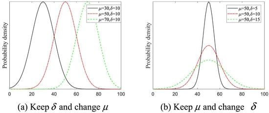
Figure 1.
Distribution values of and .
2.1.2. Local Search (Exploitation)
Based on the present placements of all solutions, local search contributes to positive solutions nearby the search space. Equation (2) represents the generalized distribution optimal for development.
where is the direction of monitoring of the ith solution at the tth iteration, is the average value of the ith solution, is the standard deviation value and is the portion of the punishment. The values of , and can be determined as follows.
where a, b, and are random numbers, is the best obtained values, and M is the average of the candidate solutions. M is determined using Equation (6).
2.1.3. Global Search (Exploration)
Global search is a technique for exploring a search space worldwide in order to find promising locations, as seen below.
where and are handled by the normal distribution, is random value, and and are two areas of values determined by Equation (8).
where , , and are three random numbers [1 N], which meet ≠≠≠i.
2.1.4. The Updating Mechanism of GND
The following mathematical depicts the GND’s update process.
The GND technique is described in Algorithm 1.
| Algorithm 1: Pseudo-code of the GND. |
|
2.2. Dwarf Mongoose Optimization Algorithm (DMOA)
The original Dwarf Mongoose Optimization Algorithm (DMOA) design is presented [22]. The suggested DMOA replicates the dwarf mongoose’s compensating behavioral response, which is modeled as follows.
2.2.1. Alpha Group
The efficiency of each solution is calculated after the population has been initiated. Equation (11) calculates the likelihood value, and the alpha female is chosen based on this likelihood.
The relates to the number of mongooses in the . Where, is the number of babysitters, is the vocalization of the dominant female that maintains the family on track [22]. The solutions updating mechanism is given as follows.
where is a distributed random number. The sleeping mound is as provided in Equation (13) but after every repetition, where phi is a uniformly distributed random integer [1, 1].
Equation (14) gives the average number of the sleeping mound discovered.
Once the babysitting exchange criterion is fulfilled, the algorithm advances to the scouting stage, when the next food supply or resting mound is considered.
2.2.2. Scout Group
In the scout group part, if the family forages quite far, they will come across a good sleeping mound. The scout mongoose is simulated by Equation (15).
where, is a random value in range [0, 1], value is calculated by Equation (16), and value is calculated by Equation (17).
Babysitters are generally inferior group members that stay with the youngsters and are cycled on a routine basis to enable the alpha female (mother) to conduct the rest of the squad on daily hunting expeditions.
The DMOA technique is described in Algorithm 2.
| Algorithm 2: Pseudo-code of the DMOA. |
|
2.3. Opposition-Based Learning (OBL) Mechanism
This section introduces the Opposition-based Learning Algorithm (OBL). It is utilized to create a new opposing solution based on the previous one [70].
In the OBL, an opposite solution () is presented as a real number. X∈ [,] is determined by Equation (18).
Opposite value: X = (, , …, ) is a within the given range, {} and [], j∈ 1, 2, …, D. This mathematical is utilized by Equation (19).
The fitness function evaluates the two solutions ( and X) during the optimization process. The best solution is identified, and the other solution is disregarded.
3. The Proposed Method (GNDDMOA)
This section introduces the suggested GNDDMOA (Generalized Normal Distribution Dwarf Mongoose Optimization Algorithm). Three basic search processes are employed to upgrade the alternatives in the suggested technique procedures. As a result of this strategy, the optimal solution will be more effective in locating a new search area and avoiding local optimum issues, such as premature, rapid, and sluggish convergence. Generalized Normal Distribution Optimization (GND), Dwarf Mongoose Optimization Algorithm (DMOA), and Opposition-based Learning (OBL) Strategies are the key procedures employed. The Standard Generalized Normal Distribution Optimization (GND) and Dwarf Mongoose Optimization Algorithm are used to discovering the best solution and improve their performance.
The Generalized Normal Distribution Optimization search methods are used in the first initialization step, followed by the Dwarf Mongoose Optimization Algorithm (DMOA) in the second initialization step, and the Opposition-based Learning (OBL) technique in the third iteration process. The Dwarf Mongoose Optimization Algorithm is put up in the second optimization period to ensure the GND by regulating the diversity of solutions and the consistency of the search methods (exploration and exploitation). The Opposition-based Learning mechanism aids the GND in the third iteration process, avoids the local optimum conundrum, and strengthens the suggested method’s ability to uncover new search regions.
The primary techniques used in the proposed GNDDMOA method, which employs integrated search techniques, are depicted in Figure 2. The main proposed conditions are used to help handle the search process and avoid the main weaknesses of the original methods, such as being trapped in local optima and the balance between the optimization processes. The number of fitness evaluations is the same as the first method’s criteria. Therefore one fitness evaluation is conducted per iteration. As a result, the suggested GNDDMOA performs one search for every repeat from the used technicians: GND, DMOA, or OBL. As a result, the suggested GNDDMOA is intended to address the core approaches’ major flaws and inadequacies in order to identify plausible solutions to the presented optimization and data clustering challenges.
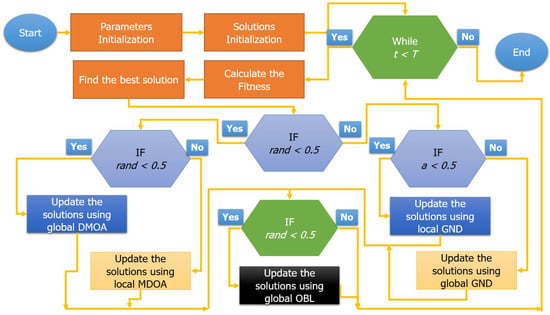
Figure 2.
The proposed GNDDMOA method.
Complexity of the Proposed GGNDDMOA
The complexity of the proposed GGNDDMOA depends on the complexity of traditional GGN, DMOA, and OBL. The total complexity is given as:
Therefore, the complexity of GGNDDMOA is given as:
The best case of the proposed GGNDDMOA is as follows:
The worst case of the proposed GGNDDMOA is as follows:
where is the number of solutions.
4. Experiments and Results
This section presents the experiments that were conducted to test the performance of the proposed method and to compare it with other methods. The experiments are divided into two main parts: benchmark functions and data clustering problems.
4.1. Experiments 1: Benchmark Functions Problems
The findings of the functions that were tested, as well as their explanations, are presented in this section. The obtained GNDDMOA findings were compared to those of well-known optimization methods, such as Aquila Optimizer (AO) [25], Salp Cosine Algorithm (SSA) [71], Particle Swarm optimizer (PSO) [72], Generalized Normal Distribution (GND) [23], Ebola Optimization Search Algorithm (AOSA) [29], Dragonfly Algorithm (DA) [73], Reptile Search Algorithm (RSA) [27], Whale Optimization Algorithm (WOA) [74], Grey Wolf Optimizer (GWO) [75], Arithmetic Optimization Algorithm [24], and Dwarf Mongoose Optimization Algorithm (DMOA) [22]. The suggested method’s performance was validated using the Friedman ranking test and the Wilcoxon ranking test. Using the Matlab program, Windows 10, and 16 GB RAM, all tests were performed 20 times [76] with the same number of iterations (1000).
4.1.1. Details of the Tested Benchmark Function Problems
Table 1 shows the system parameters for the algorithms that were tested. Table 2 shows the outcomes of the test functions that were tested.

Table 1.
Parameter values of the tested algorithms.
Table 2.
Details of the tested benchmark functions.
4.1.2. Test Function Problems
Figure 3 shows the research function issues’ qualitative findings (F1–F13). Each row has four key sub-figures: function topology, first-dimension trajectory, average fitness values, and convergence curves. In virtually all of the examined scenarios, it is evident that the recommended strategy provided the optimum result. The optimization technique is quite efficient, as evidenced by the trajectory of the selected dimension, which alters the position values substantially.
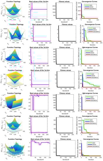
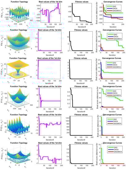
Figure 3.
Qualitative results for the tested 13 problems (F1–F13).
The population size is examined in Table 3 to determine the appropriate number of solutions to employ in the suggested technique. The best size was 50 since it received the highest ranking. As indicated in Table 4, the first 13 benchmark functions (F1–F13) were assessed using ten dimensions. Compared to existing comparable methodologies, the suggested GNDDMOA method yielded better results in this table. AO, EO, AOA, GWO, PSO, WOA, GND, SCA, SSA, ALO, and DA were placed second and third, respectively. Almost all of the examined functions yielded promising results using the suggested technique. We examined the first of the 13 benchmark functions and compared them to previous approaches—the suggested GNDDMOA method yielded more accurate results. The GNDDMOA suggested approach produced excellent or outstanding results in virtually all of the high-dimensional functions examined. Table 5 shows the results of the second ten benchmark functions (F14–F23). The suggested GNDDMOA approach also outperformed other comparable methods in this table. PSO, SSA, GWO, ALO, EO, AO, GND, DA, WOA, SCA, and AOA were placed second and third, respectively. In practically every function examined, the recommended technique yielded the best results. Furthermore, the suggested strategy outperformed the SSA, DA, and EO methods in the Wilcoxon ranking test. The Wilcoxon ranking test revealed that the suggested technique outperformed SSA, DA, EO, and GND in the first benchmark case (F1). The final ranking is presented in Figure 4.
Table 3.
The effect of the number of solutions (N) on the performance of the proposed method.
Table 4.
The results of the comparative algorithms using 13 problems, where the dimension was 10.
Table 5.
The results of the comparative algorithms using 10 problems.
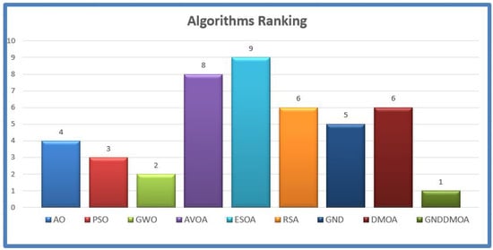
Figure 4.
The ranking results of the tested methods overall for the tested functions.
The convergence behavior of the comparison approaches is shown in Figure 5 to depict the performance curves clearly. Specifically, the suggested GNDDMOA approach smoothly accelerated the best solutions ahead. It definitely found the best solution in all of the challenges it was tested on (F1–F23). Furthermore, most test scenarios indicated that the proposed GNDDMOA avoided the primary flaws previously identified, such as premature convergence. In addition, as in the previous four test instances, the convergence stability was clearly visible. As a consequence of the acquired data, we determined that the suggested approach functioned very well and produced highly comparable outcomes to those of traditional techniques and other well-established approaches.
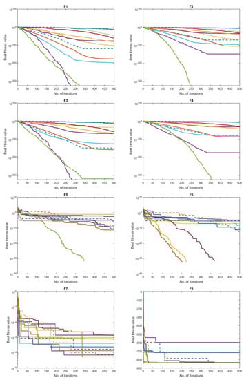
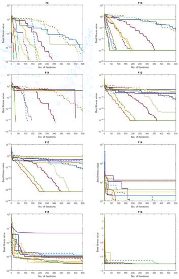
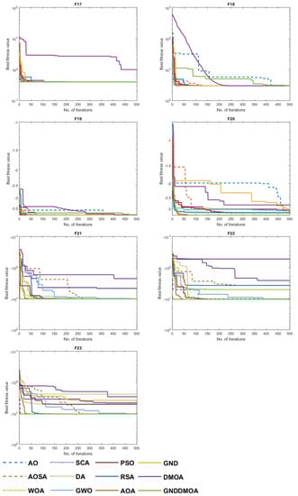
Figure 5.
Convergence behaviour of the comparative optimization algorithms on the test functions (F1–F23).
4.2. Experiments 2: Data Clustering Problems
A second phase of experiments was carried out to tackle eight data clustering difficulties and is described in this section. Table 6 contains explanations of the data clustering challenges that were evaluated. The suggested GNDDMOA’s findings were compared to those of well-known optimization methods, such as Aquila Optimizer (AO) [25], Particle Swarm optimizer (PSO) [72], Artificial Gorilla Troops Optimizer (AGTO) [77], Ebola Optimization Search Algorithm (EOSA) [29], Reptile Search Algorithm (RSA) [27], Generalized Normal Distribution (GND) [23], and Dwarf Mongoose Optimization Algorithm (DMOA) [22]. The suggested method’s performance was validated using the Friedman ranking test and the Wilcoxon ranking test. Using Matlab software, Windows 10, and 16 GB RAM, all tests were performed 20 times with the same number of iterations (1000).
Table 6.
UCI benchmark datasets.
Results and Discussion
The results of the proposed GNDDMOA on data clustering issues are reported in this section. The results of the methods compared employing eight data clustering tasks are shown in Table 7. In solving real-world data clustering challenges, the suggested technique showed promising results. In all of the scenarios that were examined, it yielded the best outcomes. The suggested GNDDMOA was ranked #1 in the Friedman ranking test, followed by PSO, GWO, AO, AOA, AGTO, GND, WOA, and AOVA. Furthermore, the Wilcoxon ranking test revealed that the suggested technique outperformed AO, PSO, GWO, AVOA, WOA, and GND in the first dataset (Cancer). Table 8, Table 9, Table 10, Table 11, Table 12, Table 13, Table 14 and Table 15 demonstrate the best values for the centroids achieved using the suggested approach.
Table 7.
The results of the comparative algorithms using eight data clustering problems.
Table 8.
Determining centroid of each cluster for the Cancer dataset.
Table 9.
Determining centroid of each cluster for the CMC dataset.
Table 10.
Determining centroid of each cluster for the Glass dataset.
Table 11.
Determining centroid of each cluster for the Iris dataset.
Table 12.
Determining centroid of each cluster for the Seeds dataset.
Table 13.
Determining centroid of each cluster for the Statlog (Heart) dataset.
Table 14.
Determining centroid of each cluster for the Vowel dataset.
Table 15.
Determining centroid of each cluster for the Wine dataset.
The convergence behavior of the comparison algorithms employing the investigated data clustering issues is depicted in Figure 6. Specifically, the suggested GNDDMOA approach smoothly accelerated the best solutions ahead. It clearly achieved the best solution in all of the tested problems. In addition, the majority of the test scenarios showed that the proposed GNDDMOA avoided prior fundamental flaws, such as premature convergence. Convergence stability was also observed, just as it was in the initial test scenarios. As a consequence of the obtained findings, we determined that the proposed approach performed admirably and generated comparable outcomes to the original techniques and other well-established methods. The clustering plot pictures produced by the proposed GNDDMOA are shown in Figure 7, where each dataset was examined using a different number of clusters (i.e., K 2, 4, and 8).
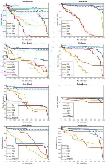
Figure 6.
Convergence behaviour of the tested methods for the data clustering applications.
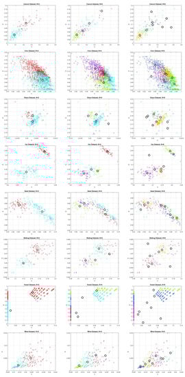
Figure 7.
Clustering plot images; each color presents a cluster (A group of data objects), and each cycle is a cluster centroid.
We chose this original method in this study as it has demonstrated its search ability in solving many challenging optimization problems. This is one of the most recent proposed methods not investigated in this domain. The main motivation bind using a new operator in the proposed method was to avoid the observed weaknesses in the original method and to make it more efficient during the optimization process.
The suggested GNDDMOA approach has a strong capacity to discover an appropriate solution to different optimization issues and data clustering, as evidenced by the previous findings and discussion. When the performance of GNDDMOA was compared to that of the classic DMOA approach, it was clear that GND and OBL had a significant impact on the capacity to balance exploration and exploitation, as seen by the excellent quality of the final solution. However, because it relies on OBL to boost processing time, the created approach still needs considerable refinement, particularly in time computation.
5. Conclusions and Potential Future Work
Recent advances in data volumes and the growth of complexity in tackling vast and complicated problems have necessitated advanced and intelligent technologies to address these issues. These approaches are usually modified procedures that enable them to cope with complex issues. Data clustering is one of the most frequent applications in the data mining industry. It is used to split a large number of data items into numerous clusters, each with several instances. The clustering method’s fundamental goal is to discover coherent clusters, with each group containing related items.
This research offers a fresh and inventive way of solving a collection of issues that require sophisticated methods to solve, based on a set of operators from several intelligent optimization algorithms. Three primary components are employed in the suggested technique (GNDDMOA) based on a unique transition mechanism to organize the executions of the used methods throughout the optimization process to address the significant flaws of the original methods. Dwarf Mongoose Optimization Algorithm (DMOA), Generalized Normal Distribution Optimization (GNF), and Opposition-based Learning Strategy are three of these strategies (OBL). The suggested transition method is utilized to implement the primary components that have been used. The suggested strategy is intended to solve the issue of premature coverage and unbalanced search strategies. The suggested method’s performance was validated using twenty-three benchmark functions and eight data clustering challenges. The proposed method’s results were compared to several other well-known methods. The suggested GNDDMOA approach produced the best results in benchmark functions and data clustering challenges in all of the evaluated scenarios. In comparison to the previous comparative methodologies, it produced good results.
The proposed method can solve other complex optimization problems in the future, such as condition monitoring, classification tasks, parameter selection, extraction of features, design issues, text grouping problems, packet headers, repairs and rehabilitation planning, and extensive medical data scheduling. In addition, a thorough examination of the suggested approach may be carried out to determine the primary reasons for the failure to identify the best solution in all circumstances.
Author Contributions
F.A.: Conceptualization, supervision, methodology, formal analysis, resources, data curation, writing–original draft preparation; L.A.: conceptualization, supervision, writing–review and editing, project administration; K.H.A.: conceptualization, supervision, methodology, formal analysis, resources, data curation, writing–original draft preparation. All authors have read and agreed to the published version of the manuscript.
Funding
The authors would like to thank the Deanship of Scientific Research at Umm Al-Qura University for supporting this work by Grant Code: (22UQU4210128DSR01).
Institutional Review Board Statement
Not Applicable.
Informed Consent Statement
Not Applicable.
Data Availability Statement
Data is available from the authors upon reasonable request.
Conflicts of Interest
The authors declare no conflict of interest.
References
- Fakhouri, H.N.; Hudaib, A.; Sleit, A. Multivector particle swarm optimization algorithm. Soft Comput. 2020, 24, 11695–11713. [Google Scholar] [CrossRef]
- Jouhari, H.; Lei, D.; Al-qaness, M.A.; Elaziz, M.A.; Damaševičius, R.; Korytkowski, M.; Ewees, A.A. Modified Harris Hawks optimizer for solving machine scheduling problems. Symmetry 2020, 12, 1460. [Google Scholar] [CrossRef]
- Abualigah, L.M.Q. Feature Selection and Enhanced Krill Herd Algorithm for Text Document Clustering; Springer: Berlin/Heidelberg, Germany, 2019. [Google Scholar]
- Abualigah, L.; Diabat, A.; Elaziz, M.A. Improved slime mould algorithm by opposition-based learning and Levy flight distribution for global optimization and advances in real-world engineering problems. J. Ambient. Intell. Humaniz. Comput. 2021, 1–40. [Google Scholar] [CrossRef]
- Abu Khurma, R.; Aljarah, I.; Sharieh, A.; Abd Elaziz, M.; Damaševičius, R.; Krilavičius, T. A review of the modification strategies of the nature inspired algorithms for feature selection problem. Mathematics 2022, 10, 464. [Google Scholar] [CrossRef]
- Hassan, M.H.; Kamel, S.; Abualigah, L.; Eid, A. Development and application of slime mould algorithm for optimal economic emission dispatch. Expert Syst. Appl. 2021, 182, 115205. [Google Scholar] [CrossRef]
- Wang, S.; Liu, Q.; Liu, Y.; Jia, H.; Abualigah, L.; Zheng, R.; Wu, D. A Hybrid SSA and SMA with Mutation Opposition-Based Learning for Constrained Engineering Problems. Comput. Intell. Neurosci. 2021, 2021, 6379469. [Google Scholar] [CrossRef]
- Attiya, I.; Abd Elaziz, M.; Abualigah, L.; Nguyen, T.N.; Abd El-Latif, A.A. An Improved Hybrid Swarm Intelligence for Scheduling IoT Application Tasks in the Cloud. IEEE Trans. Ind. Inform. 2022. [Google Scholar] [CrossRef]
- Wu, D.; Jia, H.; Abualigah, L.; Xing, Z.; Zheng, R.; Wang, H.; Altalhi, M. Enhance Teaching-Learning-Based Optimization for Tsallis-Entropy-Based Feature Selection Classification Approach. Processes 2022, 10, 360. [Google Scholar] [CrossRef]
- Damaševičius, R.; Maskeliūnas, R. Agent State Flipping Based Hybridization of Heuristic Optimization Algorithms: A Case of Bat Algorithm and Krill Herd Hybrid Algorithm. Algorithms 2021, 14, 358. [Google Scholar] [CrossRef]
- Kharrich, M.; Abualigah, L.; Kamel, S.; AbdEl-Sattar, H.; Tostado-Véliz, M. An Improved Arithmetic Optimization Algorithm for design of a microgrid with energy storage system: Case study of El Kharga Oasis, Egypt. J. Energy Storage 2022, 51, 104343. [Google Scholar] [CrossRef]
- Abualigah, L.; Almotairi, K.H.; Abd Elaziz, M.; Shehab, M.; Altalhi, M. Enhanced Flow Direction Arithmetic Optimization Algorithm for mathematical optimization problems with applications of data clustering. Eng. Anal. Bound. Elem. 2022, 138, 13–29. [Google Scholar] [CrossRef]
- Ezugwu, A.E.; Ikotun, A.M.; Oyelade, O.O.; Abualigah, L.; Agushaka, J.O.; Eke, C.I.; Akinyelu, A.A. A comprehensive survey of clustering algorithms: State-of-the-art machine learning applications, taxonomy, challenges, and future research prospects. Eng. Appl. Artif. Intell. 2022, 110, 104743. [Google Scholar] [CrossRef]
- Al-qaness, M.A.; Ewees, A.A.; Fan, H.; Abualigah, L.; Abd Elaziz, M. Boosted ANFIS model using augmented marine predator algorithm with mutation operators for wind power forecasting. Appl. Energy 2022, 314, 118851. [Google Scholar] [CrossRef]
- Mahajan, S.; Abualigah, L.; Pandit, A.K.; Altalhi, M. Hybrid Aquila optimizer with arithmetic optimization algorithm for global optimization tasks. Soft Comput. 2022, 26, 4863–4881. [Google Scholar] [CrossRef]
- Hussein, A.M.; Rashid, N.A.; Abdulah, R. Parallelisation of maximal patterns finding algorithm in biological sequences. In Proceedings of the 2016 3rd International Conference on Computer and Information Sciences (ICCOINS), Kuala Lumpur, Malaysia, 15–17 August 2016; pp. 227–232. [Google Scholar]
- Abbassi, A.; Ben Mehrez, R.; Bensalem, Y.; Abbassi, R.; Kchaou, M.; Jemli, M.; Abualigah, L.; Altalhi, M. Improved Arithmetic Optimization Algorithm for Parameters Extraction of Photovoltaic Solar Cell Single-Diode Model. Arab. J. Sci. Eng. 2022, 1–17. [Google Scholar] [CrossRef]
- De la Torre, R.; Corlu, C.G.; Faulin, J.; Onggo, B.S.; Juan, A.A. Simulation, optimization, and machine learning in sustainable transportation systems: Models and applications. Sustainability 2021, 13, 1551. [Google Scholar] [CrossRef]
- Hussein, A.M.; Abdullah, R.; AbdulRashid, N.; Ali, A.N.B. Protein multiple sequence alignment by basic flower pollination algorithm. In Proceedings of the 2017 8th International Conference on Information Technology (ICIT), Amman, Jordan, 17–18 May 2017; pp. 833–838. [Google Scholar]
- Nadimi-Shahraki, M.H.; Taghian, S.; Mirjalili, S.; Ewees, A.A.; Abualigah, L.; Abd Elaziz, M. MTV-MFO: Multi-Trial Vector-Based Moth-Flame Optimization Algorithm. Symmetry 2021, 13, 2388. [Google Scholar] [CrossRef]
- Fan, C.L. Evaluation of Classification for Project Features with Machine Learning Algorithms. Symmetry 2022, 14, 372. [Google Scholar] [CrossRef]
- Agushaka, J.O.; Ezugwu, A.E.; Abualigah, L. Dwarf mongoose optimization algorithm. Comput. Methods Appl. Mech. Eng. 2022, 391, 114570. [Google Scholar] [CrossRef]
- Zhang, Y.; Jin, Z.; Mirjalili, S. Generalized normal distribution optimization and its applications in parameter extraction of photovoltaic models. Energy Convers. Manag. 2020, 224, 113301. [Google Scholar] [CrossRef]
- Abualigah, L.; Diabat, A.; Mirjalili, S.; Abd Elaziz, M.; Gandomi, A.H. The arithmetic optimization algorithm. Comput. Methods Appl. Mech. Eng. 2021, 376, 113609. [Google Scholar] [CrossRef]
- Abualigah, L.; Yousri, D.; Abd Elaziz, M.; Ewees, A.A.; Al-qaness, M.A.; Gandomi, A.H. Aquila Optimizer: A novel meta-heuristic optimization Algorithm. Comput. Ind. Eng. 2021, 157, 107250. [Google Scholar] [CrossRef]
- He, S.; Wu, Q.H.; Saunders, J. Group search optimizer: An optimization algorithm inspired by animal searching behavior. IEEE Trans. Evol. Comput. 2009, 13, 973–990. [Google Scholar] [CrossRef]
- Abualigah, L.; Abd Elaziz, M.; Sumari, P.; Geem, Z.W.; Gandomi, A.H. Reptile Search Algorithm (RSA): A nature-inspired meta-heuristic optimizer. Expert Syst. Appl. 2022, 191, 116158. [Google Scholar] [CrossRef]
- Ahmadianfar, I.; Bozorg-Haddad, O.; Chu, X. Gradient-based optimizer: A new metaheuristic optimization algorithm. Inf. Sci. 2020, 540, 131–159. [Google Scholar] [CrossRef]
- Oyelade, O.N.; Ezugwu, A.E.S.; Mohamed, T.I.; Abualigah, L. Ebola Optimization Search Algorithm: A New Nature-Inspired Metaheuristic Optimization Algorithm. IEEE Access 2022, 10, 16150–16177. [Google Scholar] [CrossRef]
- Askarzadeh, A. Bird mating optimizer: An optimization algorithm inspired by bird mating strategies. Commun. Nonlinear Sci. Numer. Simul. 2014, 19, 1213–1228. [Google Scholar] [CrossRef]
- Hussein, A.M.; Abdullah, R.; AbdulRashid, N. Flower Pollination Algorithm With Profile Technique For Multiple Sequence Alignment. In Proceedings of the 2019 IEEE Jordan International Joint Conference on Electrical Engineering and Information Technology (JEEIT), Amman, Jordan, 9–11 April 2019; pp. 571–576. [Google Scholar]
- Wang, B.; Jin, X.; Cheng, B. Lion pride optimizer: An optimization algorithm inspired by lion pride behavior. Sci. China Inf. Sci. 2012, 55, 2369–2389. [Google Scholar] [CrossRef]
- Dehghani, M.; Montazeri, Z.; Givi, H.; Guerrero, J.M.; Dhiman, G. Darts game optimizer: A new optimization technique based on darts game. Int. J. Intell. Eng. Syst 2020, 13, 286–294. [Google Scholar] [CrossRef]
- MiarNaeimi, F.; Azizyan, G.; Rashki, M. Multi-level cross entropy optimizer (MCEO): An evolutionary optimization algorithm for engineering problems. Eng. Comput. 2018, 34, 719–739. [Google Scholar] [CrossRef]
- Khodadadi, N.; Azizi, M.; Talatahari, S.; Sareh, P. Multi-Objective Crystal Structure Algorithm (MOCryStAl): Introduction and Performance Evaluation. IEEE Access 2021, 9, 117795–117812. [Google Scholar] [CrossRef]
- Kaveh, A.; Talatahari, S.; Khodadadi, N. Stochastic paint optimizer: Theory and application in civil engineering. Eng. Comput. 2020, 1–32. [Google Scholar] [CrossRef]
- Pan, J.S.; Lv, J.X.; Yan, L.J.; Weng, S.W.; Chu, S.C.; Xue, J.K. Golden eagle optimizer with double learning strategies for 3D path planning of UAV in power inspection. Math. Comput. Simul. 2022, 193, 509–532. [Google Scholar] [CrossRef]
- Zamani, H.; Nadimi-Shahraki, M.H.; Gandomi, A.H. QANA: Quantum-based avian navigation optimizer algorithm. Eng. Appl. Artif. Intell. 2021, 104, 104314. [Google Scholar] [CrossRef]
- Zamani, H.; Nadimi-Shahraki, M.H.; Gandomi, A.H. CCSA: Conscious neighborhood-based crow search algorithm for solving global optimization problems. Appl. Soft Comput. 2019, 85, 105583. [Google Scholar] [CrossRef]
- Nadimi-Shahraki, M.H.; Taghian, S.; Mirjalili, S. An improved grey wolf optimizer for solving engineering problems. Expert Syst. Appl. 2021, 166, 113917. [Google Scholar] [CrossRef]
- Abdullah, J.M.; Ahmed, T. Fitness dependent optimizer: Inspired by the bee swarming reproductive process. IEEE Access 2019, 7, 43473–43486. [Google Scholar] [CrossRef]
- Zhao, W.; Wang, L.; Mirjalili, S. Artificial hummingbird algorithm: A new bio-inspired optimizer with its engineering applications. Comput. Methods Appl. Mech. Eng. 2022, 388, 114194. [Google Scholar] [CrossRef]
- Dehghani, M.; Montazeri, Z.; Malik, O.P. DGO: Dice game optimizer. Gazi Univ. J. Sci. 2019, 32, 871–882. [Google Scholar] [CrossRef] [Green Version]
- Askari, Q.; Younas, I.; Saeed, M. Political Optimizer: A novel socio-inspired meta-heuristic for global optimization. Knowl.-Based Syst. 2020, 195, 105709. [Google Scholar] [CrossRef]
- Azizyan, G.; Miarnaeimi, F.; Rashki, M.; Shabakhty, N. Flying Squirrel Optimizer (FSO): A novel SI-based optimization algorithm for engineering problems. Iran. J. Optim. 2019, 11, 177–205. [Google Scholar]
- Dehghani, M.; Hubálovskỳ, Š.; Trojovskỳ, P. Cat and Mouse Based Optimizer: A New Nature-Inspired Optimization Algorithm. Sensors 2021, 21, 5214. [Google Scholar] [CrossRef] [PubMed]
- Zamani, H.; Nadimi-Shahraki, M.H.; Gandomi, A.H. Starling murmuration optimizer: A novel bio-inspired algorithm for global and engineering optimization. Comput. Methods Appl. Mech. Eng. 2022, 392, 114616. [Google Scholar] [CrossRef]
- Jiang, Y.; Wu, Q.; Zhu, S.; Zhang, L. Orca predation algorithm: A novel bio-inspired algorithm for global optimization problems. Expert Syst. Appl. 2021, 188, 116026. [Google Scholar] [CrossRef]
- Sharma, B.; Hashmi, A.; Gupta, C.; Khalaf, O.I.; Abdulsahib, G.M.; Itani, M.M. Hybrid Sparrow Clustered (HSC) Algorithm for Top-N Recommendation System. Symmetry 2022, 14, 793. [Google Scholar] [CrossRef]
- Alotaibi, Y. A New Meta-Heuristics Data Clustering Algorithm Based on Tabu Search and Adaptive Search Memory. Symmetry 2022, 14, 623. [Google Scholar] [CrossRef]
- Ahmadi, R.; Ekbatanifard, G.; Bayat, P. A Modified Grey Wolf Optimizer Based Data Clustering Algorithm. Appl. Artif. Intell. 2021, 35, 63–79. [Google Scholar] [CrossRef]
- Esmin, A.A.; Coelho, R.A.; Matwin, S. A review on particle swarm optimization algorithm and its variants to clustering high-dimensional data. Artif. Intell. Rev. 2015, 44, 23–45. [Google Scholar] [CrossRef]
- Vats, S.; Sagar, B.B.; Singh, K.; Ahmadian, A.; Pansera, B.A. Performance evaluation of an independent time optimized infrastructure for big data analytics that maintains symmetry. Symmetry 2020, 12, 1274. [Google Scholar] [CrossRef]
- Abualigah, L. Group search optimizer: A nature-inspired meta-heuristic optimization algorithm with its results, variants, and applications. Neural Comput. Appl. 2021, 33, 2949–2972. [Google Scholar] [CrossRef]
- Abualigah, L.; Gandomi, A.H.; Elaziz, M.A.; Hussien, A.G.; Khasawneh, A.M.; Alshinwan, M.; Houssein, E.H. Nature-inspired optimization algorithms for text document clustering—A comprehensive analysis. Algorithms 2020, 13, 345. [Google Scholar] [CrossRef]
- Jung, Y.; Park, H.; Du, D.Z.; Drake, B.L. A decision criterion for the optimal number of clusters in hierarchical clustering. J. Glob. Optim. 2003, 25, 91–111. [Google Scholar] [CrossRef]
- Huang, D.; Wang, C.D.; Lai, J.H.; Kwoh, C.K. Toward multidiversified ensemble clustering of high-dimensional data: From subspaces to metrics and beyond. IEEE Trans. Cybern. 2021, 1–14. [Google Scholar] [CrossRef] [PubMed]
- Huang, D.; Wang, C.D.; Peng, H.; Lai, J.; Kwoh, C.K. Enhanced ensemble clustering via fast propagation of cluster-wise similarities. IEEE Trans. Syst. Man, Cybern. Syst. 2018, 51, 508–520. [Google Scholar] [CrossRef]
- Steinbach, M.; Ertöz, L.; Kumar, V. The challenges of clustering high dimensional data. In New Directions in Statistical Physics; Springer: Berlin/Heidelberg, Germany, 2004; pp. 273–309. [Google Scholar]
- Steinley, D. K-means clustering: A half-century synthesis. Br. J. Math. Stat. Psychol. 2006, 59, 1–34. [Google Scholar] [CrossRef] [Green Version]
- Guo, W.; Xu, P.; Dai, F.; Hou, Z. Harris hawks optimization algorithm based on elite fractional mutation for data clustering. Appl. Intell. 2022, 1–27. [Google Scholar] [CrossRef]
- Almotairi, K.H.; Abualigah, L. Hybrid Reptile Search Algorithm and Remora Optimization Algorithm for Optimization Tasks and Data Clustering. Symmetry 2022, 14, 458. [Google Scholar] [CrossRef]
- Abualigah, L.; Gandomi, A.H.; Elaziz, M.A.; Hamad, H.A.; Omari, M.; Alshinwan, M.; Khasawneh, A.M. Advances in meta-heuristic optimization algorithms in big data text clustering. Electronics 2021, 10, 101. [Google Scholar] [CrossRef]
- Singh, T.; Saxena, N.; Khurana, M.; Singh, D.; Abdalla, M.; Alshazly, H. Data clustering using moth-flame optimization algorithm. Sensors 2021, 21, 4086. [Google Scholar] [CrossRef]
- Wang, B.; Wang, Y.; Hou, J.; Li, Y.; Guo, Y. Open-Set source camera identification based on envelope of data clustering optimization (EDCO). Comput. Secur. 2022, 113, 102571. [Google Scholar] [CrossRef]
- Singh, T. A novel data clustering approach based on whale optimization algorithm. Expert Syst. 2021, 38, e12657. [Google Scholar] [CrossRef]
- Babu, S.S.; Jayasudha, K. A Simplex Method-Based Bacterial Colony Optimization for Data Clustering. In Innovative Data Communication Technologies and Application; Springer: Berlin/Heidelberg, Germany, 2022; pp. 987–995. [Google Scholar]
- Huang, S.; Kang, Z.; Xu, Z.; Liu, Q. Robust deep k-means: An effective and simple method for data clustering. Pattern Recognit. 2021, 117, 107996. [Google Scholar] [CrossRef]
- Deeb, H.; Sarangi, A.; Mishra, D.; Sarangi, S.K. Improved Black Hole optimization algorithm for data clustering. J. King Saud. Univ. Comput. Inf. Sci. 2020; in press. [Google Scholar] [CrossRef]
- Tizhoosh, H.R. Opposition-based learning: A new scheme for machine intelligence. In Proceedings of the International Conference on Computational Intelligence for Modelling, Control and Automation and International Conference on Intelligent Agents, Web Technologies and Internet Commerce (CIMCA-IAWTIC’06), Vienna, Austria, 28–30 November 2005; Volume 1, pp. 695–701. [Google Scholar]
- Mirjalili, S. SCA: A sine cosine algorithm for solving optimization problems. Knowl.-Based Syst. 2016, 96, 120–133. [Google Scholar] [CrossRef]
- Shi, Y.; Eberhart, R. A modified particle swarm optimizer. In Proceedings of the 1998 IEEE International Conference on Evolutionary Computation Proceedings, IEEE World Congress on Computational Intelligence (Cat. No. 98TH8360), Anchorage, AK, USA, 4–9 May 1998; pp. 69–73. [Google Scholar]
- Mirjalili, S. Dragonfly algorithm: A new meta-heuristic optimization technique for solving single-objective, discrete, and multi-objective problems. Neural Comput. Appl. 2016, 27, 1053–1073. [Google Scholar] [CrossRef]
- Mirjalili, S.; Lewis, A. The whale optimization algorithm. Adv. Eng. Softw. 2016, 95, 51–67. [Google Scholar] [CrossRef]
- Mirjalili, S.; Mirjalili, S.M.; Lewis, A. Grey wolf optimizer. Adv. Eng. Softw. 2014, 69, 46–61. [Google Scholar] [CrossRef] [Green Version]
- Jäntschi, L. A test detecting the outliers for continuous distributions based on the cumulative distribution function of the data being tested. Symmetry 2019, 11, 835. [Google Scholar] [CrossRef] [Green Version]
- Abdollahzadeh, B.; Soleimanian Gharehchopogh, F.; Mirjalili, S. Artificial gorilla troops optimizer: A new nature-inspired metaheuristic algorithm for global optimization problems. Int. J. Intell. Syst. 2021, 36, 5887–5958. [Google Scholar] [CrossRef]
Publisher’s Note: MDPI stays neutral with regard to jurisdictional claims in published maps and institutional affiliations. |
© 2022 by the authors. Licensee MDPI, Basel, Switzerland. This article is an open access article distributed under the terms and conditions of the Creative Commons Attribution (CC BY) license (https://creativecommons.org/licenses/by/4.0/).