Article

The Application of the Modified Prim’s Algorithm to Restore the Power System Using Renewable Energy Sources

Electrical Power Engineering Institute, Warsaw University of Technology, Koszykowa Street 75, 00-662 Warsaw, Poland
*
Author to whom correspondence should be addressed.
Symmetry 2022, 14(5), 1012; https://doi.org/10.3390/sym14051012
Submission received: 10 March 2022 / Revised: 18 April 2022 / Accepted: 12 May 2022 / Published: 16 May 2022

Abstract

:
The recent trends in the development of power systems are focused on the Self-Healing Grid technology fusing renewable energy sources. In the event of a failure of the power system, automated distribution grids should continue to supply energy to consumers. Unfortunately, there are currently a limited number of algorithms for rebuilding a power system with renewable energy sources. This problem is possible to solve by implementing restoration algorithms based on graph theory. This article presents the new modification of Prim’s algorithm, which has been adapted to operate on a power grid containing several power sources, including renewable energy sources. This solution is unique because Prim’s algorithm is ultimately dedicated to single-source graph topologies, while the proposed solution is adapted to multi-source topologies. In the algorithm, the power system is modeled by the adjacency matrices. The adjacency matrixes for the considered undirected graphs are symmetric. The novel logic is based on the original method of determining weights depending on active power, reactive power and active power losses. The developed solution was verified by performing a simulation on a test model of the distribution grid powered by a renewable energy source. The control logic concept was compared with the reference algorithms, which were chosen from the ideas representing available approaches based on graph theory present in the scientific publications. The conducted research confirmed the effectiveness and validity of the novel restoration strategy. The presented algorithm may be applied as a restoration logic dedicated to power distribution systems.

1. Introduction

The presence of renewable energy sources in the power system and the requirements of reliability in electrical energy supply imply the need for continuous development in the area of automation [1]. In addition to innovative solutions in the field of equipment and controllers, algorithms are extremely important, as they are responsible for the process of reconnecting consumers to the grid after a failure [2].
In electrical engineering, graph theory has a special place. This theory is applied not only in the field of electrical circuit analysis, but also in the power grid restoration algorithms [3]. Strategies based on graph theory can be divided into two types [4,5,6,7]. The first solution uses sectioning of grid topology into smaller fragments connected with power sources. In the second group of algorithms, there are logics using greedy algorithms, especially Prim’s algorithm [8].
As an example of the methods mentioned in the previous paragraph, the algorithm from [9] is used, which works in a hybrid way. This logic determines the skeleton of the network in the first stage through Prim’s algorithm, and in the second stage the power subsystems are determined. Prim’s algorithm is based on assigning weights to each power line, and the approach to this problem is contained in [10]. The application of the algorithm responsible for dividing the reconstructed network into feeder islands is possible by a logic based on a fuzzy neural network [11]. This method creates subnetworks characterized by stable operation. One of the less popular solutions is the logic using parallel systematic resampling [12]. This logic, resulting from graph theory based on graph convolutional network algorithms, can be applied to power system reconstruction [13]. The main disadvantage of this solution is its high complexity. There are also available solutions that have limited applications in the real world and this is, for example, the algorithm from [14], which is dedicated only to radial networks. The calculation efficiency is the only advantage of the logic. The main goal of the algorithms responsible for the restoration of power systems after a failure is to provide reliable access to the electricity.
The power system restoration methods developed so far [1,2,3,4,5,6,7,8,9,10,11,12,13,14,15,16,17] are dedicated to grids equipped with non-renewable energy sources. The presence of renewable energy sources in power systems requires the preparation of algorithms enabling network restoration that also take into account the kind of electricity generators [18]. Unfortunately, the number of publications dealing with the issue of logics dedicated to the restoration of a power grid supplied from renewable energy sources after a failure is limited. In [19], the algorithm designed to rebuild a power system after an islanding work, in which the loads receive electrical power also from renewable energy sources, is designed. A different approach to the problem is presented in [20], where a particle swarm optimalization algorithm is used to rebuild the grid. A similar solution is also presented in the article [21]. Furthermore, the use of energy storage systems in combination with PV power plants is studied [22]. Unfortunately, due to the significant cost of building this type of infrastructure, it is currently a theoretical issue with no prospects for application in the near future [23]. The limited number of publications in the field of restoration algorithms dedicated to cooperation with grids equipped with renewable energy sources is due to the lack of stable power supply by PV power stations or wind power plants [24].
The method of grid sectioning used for the restoration of power grids is characterized by high complexity as well as the use of additional algorithms supporting the decision-making process, including greedy algorithms [25]. In the first stage, the logic divides the existing topology into substructures related to the load, and then creates smaller power grids powered independently from separate energy sources. The resulting topologies are not interconnected. The logic based on Prim’s algorithm is characterized by a simpler methodology of operation than the method using sectioning; however, it requires appropriate adjustment to cooperate with power systems. This is due to the fact that in its original form, Prim’s algorithm is dedicated to single-source grids. As this algorithm is to be used in the power system topology supplied by more than one source, it is necessary to generalize this logic. Nevertheless, the speed of Prim’s algorithm is an extremely important advantage.
Another problem is the cooperation of the restoration algorithms with power grids powered by renewable energy sources [26]. These sources do not guarantee the access to constant power and their efficiency depends on the weather conditions [27]. This fact needs to be taken into consideration when using logics cooperating with such sources.
Technological development and the increasing presence of renewable energy sources in the power system demand the development of algorithms responsible for its restoration after emergencies. These algorithms should be characterized by reliability and short execution time. The performed operations through the control logic should guarantee the fastest possible delivery of electricity to consumers and should assure the stability of the restored power system.
The issues mentioned in the previous paragraphs imply the necessity to adapt the restoration algorithms to the cooperation with renewable energy sources through their appropriate modification. The proposal of logic applying a properly modified Prim’s algorithm is presented in the article. Additionally, the new method of calculating weights has been proposed. This method depends on the parameters characterizing power grids, i.e., active power, reactive power and active power losses. The prepared concept was verified during simulation studies. The proposed solution was compared with the reference logic, which was chosen on the basis of the analysis of the published algorithms in available scientific articles. The logic from [8] was considered the reference algorithm due to the fact that it is characterized by the advantages of solutions from [1,2,3,4,5,6,7,8,9,10,11,12,13,14,15,16,17,18,19,20,21,22,23,24,25,26,27,28,29,30,31,32,33].

2. The Presentation of the Problem

Prim’s algorithm is a logic using graph theory, which operates on the concepts of E edges and V vertices [34]. In mathematics, an undirected graph is defined as a pair: G = ( V , E ) . Mapping of the power system in the form of a graph can be realized in two ways. The first one consists of assigning the busbars to the vertices of the graph and the transmission lines to the edges. The second solution is adapted to the presence of switches in the power system, which are represented by the edges of the graph. In this case, the transmission lines are identical with vertices [35]. The presented methods of mapping the power supply grid as graphs are shown in Figure 1. In the paper, the scheme from Figure 1b is analyzed and developed.
The edges of E of graph G are assigned numerical values called weights w, which in science are related to the physical phenomenon under consideration. In the case of Prim’s algorithm used for the purposes of the power grid restoration strategy, these weights are the indicators depending on active power and reactive power. In [8], there are various mathematical dependencies that allow us to count the weights. One of the applied formulas is as follows [8]:
w k = P P S 0 + P k + P k P s
Equation (1) is related to the active power of the loads and losses of active power in the grid under the consideration. The advantage of using this equation in the modified Prim’s algorithm is its low mathematical complexity, which guarantees time-efficient calculations. The disadvantage of using this equation includes its low flexibility, which results from not taking into account the presence of reactive power in the power system. Thus, the grid topologies obtained by means of (1), are identical each time assuming that all power lines in the considered grid are technically efficient and there is no failure, e.g., short circuit.
Otherwise, the weights are expressed as the correlation between active and reactive power in the considered topology of the power system through [7]:
w k = w 1 k b 1 · p + w 2 k b 2 · ( 1 p )
Parameters w 1 k and w 2 k are expressed in the following formulas [7]:
w 1 k = P P S 0 + P k
w 2 k = | Q P S 0 + Q k |
The values of b 1 and b 2 are calculated by [7]:
b 1 = min   ( P P S 0 + P k )
b 2 = min   | Q P S 0 + Q k |
Using calculations (2) requires the specifying parameter p . For this purpose, a particle swarm optimalization (PSO) can be used, which operates according to the predefined indicators [36]. These indicators have to be adapted to the guidelines for the given restoration algorithm [37].
The disadvantages of the solution based on (2) are the lack of consideration of active power loss and high mathematical complexity compared to (1). The advantages include the relative influence of reactive power on the value of the weight representing the power line. Thanks to the presence of parameter p , it is possible to obtain different grid topologies, which indicate flexibility in applying Formula (2).
Prim’s algorithm used for the power system restoration is a modified logic in relation to its classical version [35]. The need to change this algorithm results from the fact that it has to be adapted to the topology of the power grid, which has more than one power source. Prim’s algorithm caters for a predefined set of edges with assigned weights and vertices; this generates the smallest possible sum of the edge weights with all vertices connected to each other. The resulting topology is called a minimal spanning tree. Prim’s algorithm starts with a vertex defined as a “root”. In each step, edges with the lowest possible weight are added to the structure starting from this point. An example of how Prim’s algorithm works is shown in Figure 2.
The minimum spanning tree can be determined using Kruskal’s algorithm. However, it is not applicable to power systems, because Kruskal’s algorithm starts from the node to which the line with the lowest weight is connected. As a result, Kruskal’s algorithm can connect transmission lines in such a way that they will not be energized (there will be islands of interconnected transmission lines not supplied by the power source). In the case of Prim’s algorithm, it is possible to define the node (root) from which the edges are connected, and each connected transmission line is always energized by the power source.
The other restoration algorithms based on graph theory use the method of sectioning grid topology into smaller sub-topologies that are related to energy sources. There are three phases of operation in these logics. In the first phase, called the coarsening phase, the G 0 graph is converted into smaller graphs G 1 , G 2 , , G k . The second stage, the partitioning phase, consists of assigning weights to the edges in the G k sub-graphs. In the uncoarsening and refinement phase, which is the last phase of the network topology partitioning method, the subnetwork system supplied from independent energy sources is rebuilt by merging the G k 1 , G k 2 , , G 1 , G 0 subgraphs [7]. The idea of the algorithm is presented in Figure 3.
Each of the logics described in the previous paragraphs has its advantages and disadvantages. The advantage of Prim’s algorithm over the method of grid sectioning into smaller topologies is a small complexity of logic and a fast calculation by digital systems. The complexity of the Prim’s algorithm is O ( V 2 ) , where V is the number of vertices in a graph. Prim’s algorithm complexity can be improved up to O ( E   log V )   using the Fibonacci heap, where E is number of edges. The complexity of Prim’s algorithm using the Fibonacci heap is the same as in the case of Kruskal’s algorithm. The main advantage of the sectioning method is the possibility of creating subsystems which are powered from independent energy sources.
The development of a Smart Grid technology in connection with renewable energy sources implies the emergence of novel restoration algorithms creating micro-grids [38]. The most optimal solution is to combine the advantages of Prim’s algorithm and logic based on the power system sectioning. Implementation of this type of logic is possible by introducing the generalization of Prim’s algorithm, which is applicable to multi-source systems. These modifications require dealing with several problems.
First, it is necessary to develop a mathematical dependence expressing the weights which will reflect the operation of the power system and the presence of such parameters as active power, reactive power, and active power losses in it. The second problem is the preparation of logical conditions that will allow Prim’s algorithm to cooperate with the power grid supplied from several energy sources. The last issue that has to be taken into consideration in the algorithm is the specificity of the renewed energy sources, i.e., periodical generation of electric power by them, and thus the possibility of switching between the sources supplying the loads in the microgrids.

3. The Motivation and the Article’s Contribution

The previously described facts have motivated the authors of this paper to develop a new restoration algorithm that meets the previously mentioned conditions. This publication contains the following new contributions:
(1)
The new resuscitation algorithm for power systems based on a modification of Prim’s algorithm has been developed.
(2)
The prepared logic is adapted to work with a power system that has renewable energy sources in its topology.
(3)
For the developed algorithm, the authors have prepared a new method for determining the weights, which represent the power flows in the grid.
The proposed solutions were confirmed in simulation calculations. The simulations were performed on a modified model of the New England IEEE 39-bus system and power system model prepared by the authors.

4. The Restoration Algorithm—The Assumptions and the Control Logic

The algorithm must be adapted to the grid topology in which there are renewable energy sources and more than one electricity generator. The implementation of the control logic is based on the assumptions and conditions such as permissible voltage values on the busbars, permissible values of the current transmitted by power lines, etc.

4.1. Generation Capacity of Power Plants

For each of the electricity sources, there is a mathematical description that defines the limits of the generated power to the grid. Today in the existing topologies, nuclear power plants, coal power plants, wind farms and solar power plants are the most popular energy sources.
In the case of the power plants equipped with steam turbines, the power generated by them is limited by the rules of mechanics and thermodynamics. In the case of this type of energy source, the produced electric power is determined using the following formulas [39]:
P 2 + Q 2 = S 2 ( V · I M A X ) 2
P 2 + ( Q + V 2 x d ) 2 ( E q · V x d ) 2
P ( Q + V 2 x d ) · t a n δ M A X
P G m i n P P G m a x
In the case of renewable energy sources, the power they generate depends on the weather conditions, e.g., the power produced by a solar power plant depends on the cloud cover and the power generated by a wind power plant depends on the wind speed. For a single wind turbine, the following equations and inequalities are relevant to determine the power it generates [40,41]:
P W T = { 0     i f     v v c i     P r · v v c i v r v c i       i f     v c i v v r P r     i f     v r v v c o 0     i f     v v c o
P r = 1 2 · A W T · c p · ρ a · η r · η W T · v r 3

4.2. Power System Components’ Current and Voltage Limits

In the documentation, the operator of the power system defines the permissible voltage levels on the busbars, which result directly from the technological solutions used in the considered grid [42]. In the case of currents in transmission lines, the permissible values depend on the type of line [43].
For the analyses carried out in the article, it was assumed that the permissible voltage on the busbars ranged from 0.90 p.u. to 1.05 p.u. of the rated value for a given type of grid [7]. In the case of lines, the permissible current value cannot exceed their rated value [44].

4.3. A New Approach to Weights’ Calculations for Power System Representation as a Graph

In addition to the implementation of individual transmission lines and busbars in a matrix form, the use of graph algorithms requires the assignment of numerical values to the edges called weights. For the purposes of the implemented control logic, Formula (2) was modified, assuming that the weights are determined for the modified Prim’s algorithm, which connects the edges corresponding to the loads with the greatest demand for active power. The advantage of the presented formula in comparison to Equation (2) is considering the take-off of active power occurring in the power system. The formula used to calculate the weights is as follows:
w k = w 1 * k c 1 · p 1 + w 2 * k c 2 · p 2 + w 3 * k c 3 · p 3
Parameters w 1 * k , w 2 * k , w 3 * k , c 1 , c 2 , and c 3 are determined from the following equations:
w 1 * k = P P S 0 + P k
w 2 * k = 1     | Q P S 0 + Q k + Q k |  
w 3 * k = 1 P k
c 1 = max ( P P S 0 + P k )
c 2 = 1   min   | Q P S 0 + Q k + Q k |
c 3 = 1 min   P k
In the case of parameters p 1 , p 2 , and p 3 , a simplifying equation can be used that links these quantities with each other:
p 1 + p 2 + p 3 = 1
Applying Equation (20) reduces the Formula (13) to the form:
w k = w 1 * k c 1 · p 1 + w 2 * k c 2 · p 2 + w 3 * k c 3 · ( 1 p 1 p 2 )  
The following conditions must be met by p 1 , p 2 , and p 3 :
p 1 > 0
p 2 > 0  
p 2 > 0
The determination of the numerical value for the parameters p 1 , p 2 , and p 3 is possible using optimization algorithms. In this case, an effective approach is to use the PSO method with predefined conditions such as minimization of the time needed to connect all loads or connecting all loads while minimizing active power losses in the considered power system.
The method of calculating weights according to Equation (13) is applied to find the maximum spanning tree for the analyzed graph. The maximum spanning tree and the minimum spanning tree are the structures obtained by applying Prim’s algorithm. The relation (13) was adjusted in such a way that for the created maximum spanning tree, the active power losses were minimized, or the absolute value of the reactive power consumed by the grid created in this way was as close to zero as possible. The method for obtaining the maximum spanning tree consists of connecting the edges with the highest value of weights to the nodes (in the case of determining the minimum spanning tree Prim’s algorithm connects the edges with the highest value of weights to the nodes).
The rationale for using Prim’s algorithm for determining the maximum spanning tree and Formula (13) are discussed in the example used in Figure 4. In the considered topology, the following simplifying assumptions are made:
(1)
The DC grid is the considered topology, hence in Formula (13) p 2 = 0 .
(2)
There are no active power losses in the considered grid, hence in Formula (13) p3 = 0.
The application of Prim’s algorithm determining the minimum spanning tree and Equation (13) lead to the topology of Figure 4a, where loads with the total power of 0.8 p.u. are connected to the source with the power equal to 1.0 p.u. In the case of Figure 4b, the application of Prim’s algorithm for determining the maximum spanning tree allowed the connection of loads with the power of 1.0 p.u. From the economic point of view, the largest possible sale of electrical energy is the optimal solution. In the analyzed example, the effectiveness program applying Prim’s algorithm, which creates maximal spanning tree topology, and the use of the Formula (13) was shown.

4.4. Assumptions for the Logic of the Modified Prim’s Algorithm

Prim’s algorithm is dedicated to graph structures with a single power source. Its application in the logic responsible for the reconstruction of a power system requires appropriate modifications in the following aspects:
(1)
Adaptation of Prim’s algorithm to multi-source topologies.
(2)
Implementation of logical conditions responsible for the selection of the source for which a new supply line (edge) is to be connected at a given moment.
Obtaining the grid topology in which all the loads have been powered [29] is the reason to solve the previously mentioned dilemmas. This problem is discussed on the basis of Figure 5, where it is assumed that the transmission lines do not generate power losses. A DC grid is the considered grid, and the values of the weights are calculated using Formula (13). In case where there is no predefined logic responsible for the selection of the source to which the power line is to be connected and the sources are switched in the order of their numbering, as was realized in [8], the result is a tree topology where not all sources have been supplied. The example of such a topology obtained by Prim’s algorithm, responsible for the creation of maximum spanning tree, is shown in Figure 5a, where the applied Prim’s algorithm is not optimal (one source remains unpowered).
The elimination of the tree microgrids, where the loads remain unconnected to the energy source, is possible by using the following formulas described in [45]:
n j = n a l l j n c y c l e j
α j = P s j P P S 0 j
Formula (25) is used to select the power source to which the next power line is to be connected. The connection is made to the source for which the value of the n j coefficient is as small as possible. If two or more identical, and simultaneously smallest, values of n j are obtained, then the source is selected on the basis of the n j coefficient. The power line is first connected to the source for which the largest possible value from Equation (26) was obtained. In the case where the same value has been obtained for several sources, which is at the same time the largest value of the α j , the source to which the power line should be connected is selected according to the assigned numbering, i.e., the first source in the order implemented in the program is selected. An example of the application of logic using Formulas (25) and (26) from [45] gained by the Prim’s algorithm responsible for the creation of the maximum spanning tree is presented in Figure 5b, where the obtained grid has all loads powered.
The assumptions presented in [45] are valid for the grids with non-renewable energy sources. In the case of renewable energy sources, the modified Prim’s algorithm from [45] does not allow for the proper connection of all loads to sources that do not depend on the weather conditions. The example of inappropriate and appropriate operations of the modified Prim’s algorithms is shown in Figure 6, where the considered grid is equipped with two energy sources (renewable source WT1 and non-renewable source G1). The analyses do not take into account the presence of reactive power and the power losses associated with the transmission lines. The modified Prim’s algorithm from [45] based on Equation (13) considered p 1 = 1 and p 2 = p 3 = 0 , which is used to obtain the topology of Figure 6a. The topology of Figure 6a guarantees reliable power delivery only to the loads connected to busbars BB2 and BB4. The loads from busbars BB3 and BB5 are supplied from a renewable source which depends on the weather conditions. The reduction in energy delivery at the output of the wind turbine may result in the disconnection of loads in order to ensure grid operation conditions in terms of frequency and power.
The right approach to solve this problem is to power the loads with non-renewable energy sources. This is possible because of the assumption that the renewable sources are considered by the logic in the same way as the loads nodes. This can be realized by using the numbers in the adjacency matrix. This matrix is a mathematical representation in the graphical form of a given topology that specifies what type of node the program is dealing with. Figure 6b shows the example of the obtained grid where each of the loads, as well as the renewable energy sources, are connected to each other.
The example of an adjacency matrix that is the representation of the case in Figure 6 is as follows:
L = [ 0 2 0 2 0 0 2 0 1 0 0 0 0 1 0 0 1 1 2 0 0 0 1 0 0 0 1 1 0 1 0 0 1 0 1 0 ]
In the matrix L , the number 0 indicates no transmission line between the pair of nodes; number 1 indicates the transmission line which may be connected to the nodes with loads and the transmission line which may be connected to the renewable source. The number 2 indicates the transmission line which may be connected directly to the non-renewable power sources and thus identifies the location of non-renewable power source nodes in the grid topology.
The last stage is the connection process between the microgrids obtained by using the modified Prim’s algorithm, and then connecting the other transmission lines. The order of connections is to be done according to the numbering of individual nodes. At the same time, it is necessary to check the power conditions for non-renewable power sources (it is not allowed to exceed the limits of operation power ranges for each power source).
It should be emphasized that the connections of the transmission lines occur in a predefined order that depends on the voltage level. The priority is always given to making connections for the highest voltage level and then it is done for structures with the lower voltage values.

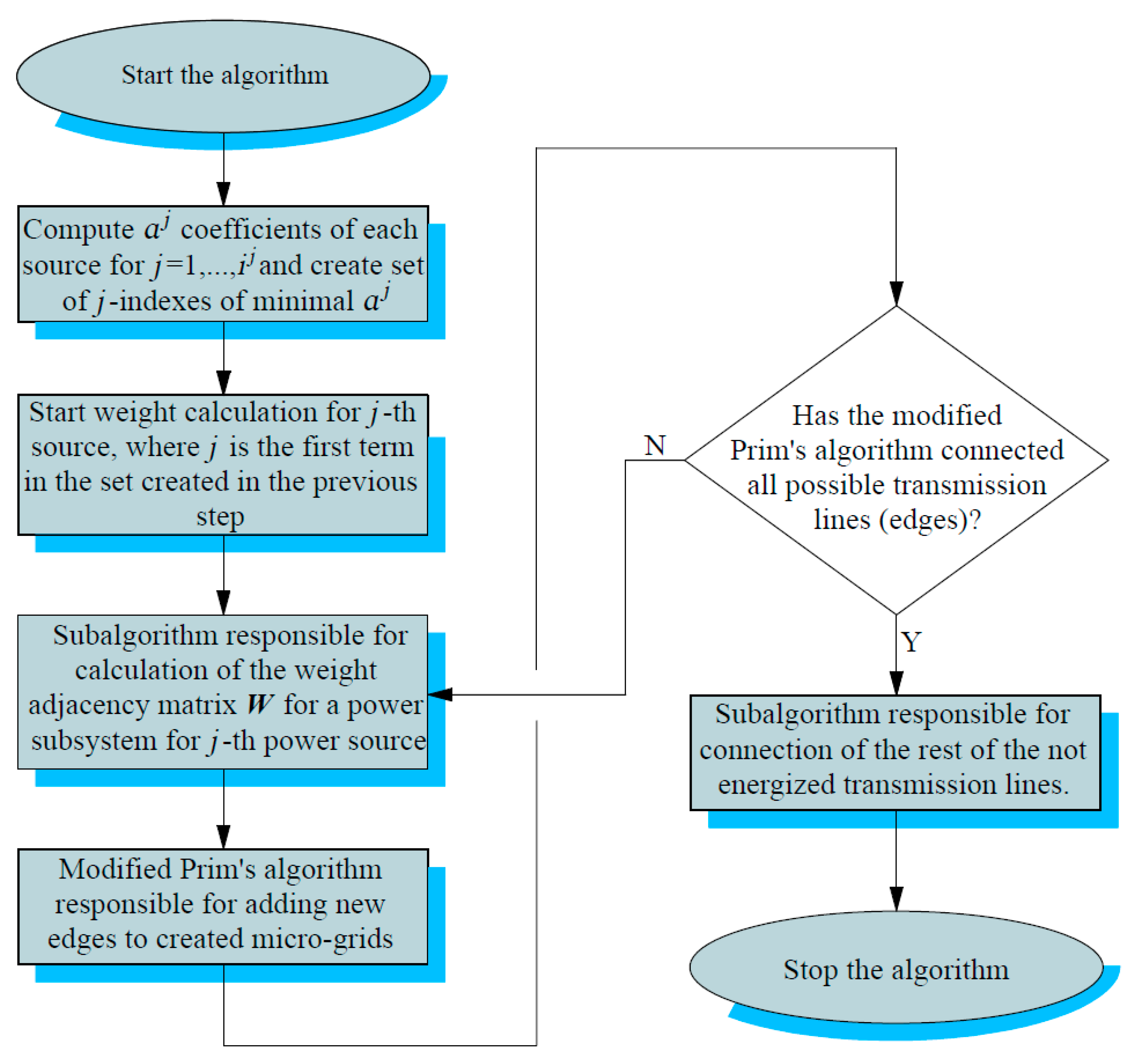
4.5. The New Power System Restoration Logic Applying the Modified Prim’s Algorithm

The logic using the modified Prim’s algorithm for the restoration of the power system is based on the assumptions presented in the previous part of the article and operates on the following matrices: α , P , Q , I P S , I r , I W , J , J * , J * * , J m i n , k w , N , Q , Q P S , P , P P S , T , V P S , V r , V W , W , W 1 , W 2 , W 3 , and Z . The structure of the developed Algorithm 1 consists of Algorithms 2–5. At the start of the algorithm, the supply nodes are energized, i.e., the supply node is understood as the connection between the generator and the transformer. The logic in the graphical form is shown in Figure 7.
Algorithm 1.Algorithm dedicated to the restoration of the power system based on the modified Prim’s algorithm.
BEGIN
VARIABLES :   α j , α j 1 ,   e ,   i j ,   j ,   j c ,   n J *   P P S 0 j ,     P s j ,     J *
e : = 0
j : = 1
n J * : = 0
J * : = [ ]
FOR   j = 1 TO   j = i j  DO
  Calculate   P s j   and   P P S 0 j
  α j : = P s j P P S 0 j
  IF   j = 1   OR   ( j > 1   AND   α j < α j 1 ) THEN
  α j 1 : = α j
  j c : = j
    END IF
  j : = j + 1
   END FOR
WHILE   e = 0
    Algorithm 1
    Algorithm 2
    Algorithm 3
   END WHILE
WHILE   e = 1
    Algorithm 4
   END WHILE
END
Algorithm 2.Algorithm responsible for weight’s calculations.
BEGIN
  VARIABLES: c 1 ,   c 2 ,   c 3 ,     P k ,     Q k ,     k ,   i j ,   i c ,     i n , i s ,   p 1 ,   p 2 , p 3 ,   P s j ,   P P S k ,   Q s j ,     Q P S k ,   v n ,   v c ,   v s ,
   P , Q , I W , k W ,   P P S , Q P S , V W , W , W 1 , W 2 , W 3 ,
   k : = 1
   c 1 : = 1
   c 2 : = 1
   c 3 : = 1
   P : = [ ]
   Q : = [ ]
   P P S : = [ ]
   Q P S : = [ ]
   W : = [ ]
   W 1 : = [ ]
   W 2 : = [ ]
   W 3 : = [ ]
  FOR  k = 1  TO  k = i j  DO
     V W : = [ ]
     I W : = [ ]
     v s : = 0
     v c : = 1
     i s : = 0
     i c : = 1
    Calculate P P S k ,     Q P S k ,     P k ,     Q k ,     V W , I W
    IF P P S k 2 + Q P S k 2 < ( P s j ) + ( Q s j )  THEN
      Q [ k ] : = Q k
      P P S [ k ] : = P P S k
      Q P S [ k ] : = Q P S k
     FOR v c = 1  TO  v n  DO
      IF V W [ v c ] < 0.9   p . u .  OR V [ v c ] > 1.05   p . u . THEN
        v s : = 1
        v c = v n + 1
      END IF
     END FOR
     IF v s = 0  THEN
      FOR i c = 1  AND i s = 0  TO  i n  DO
       IF I W [ i c ] > 1.0   p . u .  THEN
         i s : = 1
         i c = i n + 1
       END IF
      END FOR
      IF i s = 0  THEN
        P [ k ] : = P k
      ELSE
        P [ k ] : = 1
      END IF
     ELSE
        P [ k ] : = 1
     END IF
    ELSE
      P [ k ] : = 1
    END IF
    IF P k = 1  THEN
      W 1 [ k ] : = 1
      W 2 [ k ] : = 1
      W 3 [ k ] : = 1
    ELSE
      W 1 [ k ] : = P P S k P k
      W 2 [ k ] : = 1   | Q P S k |
      W 3 [ k ] : = 1 P k
    END IF
     k W [ k ] : = k
     k : = k + 1
  END FOR
   k : = 1
  FOR  k = 1  TO  i j  DO
    IF W 1 [ k ] > c 1   THEN
      c 1 : = W 1 [ k ]
    END IF
    IF W 2 [ k ] > c 1   THEN
      c 2 : = W 2 [ k ]
    END IF
    IF W 3 [ k ] > c 1   THEN
      c 3 : = W 3 [ k ]
    END IF
     k : = k + 1
  END FOR
   k : = 1
  FOR  k = 1  TO  i j  DO
    IF c 1 = 1   OR   c 2 = 1   OR   c 3 = 1  THEN
      W [ k ] : = 1
    ELSE
      W [ k ] : = W 1 [ k ] c 1 p 1 + W 2 [ k ] c 2 p 2 + W 3 [ k ] c 3 p 3
    END IF
     k : = k + 1
  END FOR
   k : = 1
END
Algorithm 3.The modified Prim’s algorithm.
BEGIN
   VARIABLES :   i j ,   j c ,   k ,   k m a x ,   n J * ,   Q ,   u ,   v ,   w ,   w m a x ,   w s ,     J * ,   T ,   W
   w s : = 0
     w m a x : = 0
   k m a x : = 0
  FOR k = 1  TO i j  DO
    IF W [ k ] > w m a x  THEN
      w m a x : = W [ k ]
      k m a x : = k
      w s : = 1
   END IF
  END FOR
  IF w s = 1  THEN
     Connect   the   k m a x -th transmission line by updating T
  ELSE
     n J * : = n J * + 1
     J * [ n J * ] = j c
  END IF
END
Algorithm 4.Algorithm responsible for the verification of a possible connection to Algorithm 2 already not energized by transmission lines.
BEGIN
   VARIABLES :   α ,   J ,   J * ,   J * * ,   J m i n ,   N ,   e ,   l 1 , l 2 ,   l 3 , l 4 ,   l 5 ,   l 6 ,   l 7 ,   α m a x ,   m ,   m J , n , n J * ,   n m i n ,
   P P S 0 j ,   P s j ,   z  
   N : = [ ]
   α : = [ ]
   m : = 1
   n : = 1
   n m i n : = 1
   α m a x : = 1
   l 1 : = 0
   l 3 : = 0
   l 4 : = 1
   l 5 : = 0
   l 6 : = 1
   l 7 : = 1
   FOR   m = 1   TO   m = m J    DO
     z : = 0
     FOR   n = 1   TO   n = n J *  DO
       IF   J [ m ] = J * [ n ]  THEN
         z : = 1
      END IF
       n : = n + 1
    END FOR
      m : = m + 1
     IF   z = 0  THEN
       l 1 : = l 1 + 1
       J * * [ l 1 ] : = J [ m ]
    END IF
  END FOR
   IF   l 1 = 0  THEN
     e : = 1
  ELSE
     FOR   l 2 = 1 TO   l 1  DO
      Calculate n j for J * * [ l 2 ]
       l 3 : = l 3 + 1
       N [ l 3 ] : = n j
       l 2 : = l 2 + 1
    END FOR
     FOR   l 4 = 1   TO   l 1  DO
       IF   n m i n = 1   A N D   N [ l 4 ] > 0 THEN
          n m i n : = N [ l 4 ]
          J m i n [ 1 ] : = J * * [ l 4 ]
       ELSE   IF   N [ l 4 ] n m i n   A N D   n m i n 0   A N D   N [ l 4 ] > 0   THEN
          n m i n : = N [ l 4 ]
          J m i n : = [ ]
            J m i n [ 1 ] : = J * * [ l 4 ]
         l 5 : = 1
       ELSE   IF   N [ l 4 ] = n m i n   THEN
          l 5 : = l 5 + 1
          J m i n [ l 5 ] = J * * [ l 4 ]
      END IF
       l 4 : = l 4 + 1
     END FOR
      IF   J m i n = [ ]  THEN
       e : = 1
      ELSE   IF   l 5 = 1   THEN
       j c = J m i n [ 1 ]
      ELSE   IF   l 5 > 1  THEN
       FOR   l 6 = 1   TO   l 5  DO
         Calculate α j for J m i n [ l 6 ]
          α [ l 6 ] : = α j
          l 6 : = l 6 + 1
      END FOR
       FOR   l 7 = 1   TO   l 5  DO
         IF α [ l 7 ] > α m a x  THEN
            α m a x : = α [ l 7 ]
            j c J m i n [ l 7 ]
            l 7 : = l 7 + 1
         END IF
      END FOR
    END IF
  END IF
END
Algorithm 5.Algorithm responsible for connection transmission lines not energized by Algorithm 4.
BEGIN
   VARIABLES :   b P Q ,   i c ,   i n ,   i s ,   j ,   j a l l , n c ,   n a l l ,   n n e ,   v c ,   v n ,   v s ,   P s j ,   P P S j ,   Q s j , Q P S j , I P S ,   V P S
   n n e : = 1
   n c : = 0
  Calculate n a l l
   IF   n a l l 0  THEN
     FOR n n e = 1   TO   n n e = n a l l  DO
        b P Q : = 0
        v s : = 1
        i s : = 1
        j : = 1
       FOR j = 1   A N D   b P Q = 0 TO j = j a l l  DO
          Calculate   P P S j   and Q P S j
         IF ( P P S j ) + ( Q P S j ) < ( P s j ) + ( Q s j )  AND b P Q = 0  THEN
            b P Q : = 0
            j : = j + 1
         ELSE
            b P Q : = 1
         END IF
       END FOR
       IF b P Q = 0  THEN
         Calculate V P S
          v s : = 0
          v c : = 1
         FOR v c = 1   A N D   v s = 0   T O   v n   D O
           IF V P S [ v c ] < 0.9   p . u .  OR V P S [ v c ] > 1.05   p . u .  THEN
              v s : = 1
              v c : = v n + 1
           END IF
            v c : = v c + 1
         END FOR
       END IF
       IF v s = 0  THEN
         Calculate I P S
          i s = 0
          i c : = 1
         FOR i c = 1  TO  i n  DO
           IF I P S [ i c ] > 1.0   p . u .  AND i s = 0 THEN
              i s : = 1
              i c : = i n + 1
           END IF
            i c : = i c + 1
         END FOR
       END IF
       IF i s = 0  THEN
         Connect the n n e -th transmission line by updating T
          n c : = n c + 1
       END IF
        n n e : = n n e + 1
       IF n a l l = n c  OR  n c = 0  THEN
          n n e : = n a l l + 1
       ELSE IF n n e = n a l l  THEN
          n n e : = 1
          n c : = 0
         Calculate n a l l
       END IF
    END FOR
  END IF
END

5. The Test of the Logic Based on the Modified Prim’s Algorithm

The logic based on the modified Prim’s algorithm dedicated to the restoration of the power system after a malfunction was verified on test benchmarks. The solution described in [8] was used as the reference logic to compare with the presented control algorithm in the paper. The first reference logic was considered to be the study from [8] due to the significant recognition of this article through the citations currently amounting to over 90 cross-references in the various publications. The second reference logic is from the recent research article [45].

5.1. Power System Test Benchmarks

The tests of the designed restoration logic using the modified Prim’s algorithm were conducted on two test power system benchmarks. The first topology dedicated to computer simulations is a modified IEEE 39-bus system known as 10-machine New-England Power System, and the second case is a power system topology prepared by the authors of this article.

5.1.1. Modified IEEE 39-Bus System

The electrical power system used for simulation purposes has been modified to perform a simulation to verify the applicability of the prepared algorithm [46]. The scope of the changes to the IEEE 39-bus system is as follows [46]:
(1)
Transmission lines L06–07, L16–19, L16–24, L21–22, L22–23, L23–24 are redefined from single lines to two parallel lines with type and length according to the standard from [30]. The purpose of the change is to increase the transmission capacity of the mentioned lines in case of switching off, e.g., in line L21–22, a part of the energized lines (L16–24, L22–23, L23–24) is overloaded (transmitted current is higher than the rated value for a transmission line).
(2)
A renewable energy source in the form of wind power plants with the rated apparent power of 600 MVA, a power factor of 0.85 and a nominal voltage of 345 kVA are connected to the following busbars: BB14, BB17, and BB28.
The modified IEEE 39-bus system is shown in Figure 8.

5.1.2. Power System Test Topology Designed by the Authors

The power system used for the tests is shown in Figure 9. It consists of 27 transmission lines, 3 non-renewable energy sources, 3 renewable energy sources, 20 buses, and 17 loads. The benchmark is the topology operating at 20 kV. The data adopted for the transmission lines and loads are gathered in Table 1 and Table 2, respectively. The following assumptions were made for the test model:
(1)
All supply lines have the cross-section equal to 240 mm2, their rated current is 425 A, resistance per unit R L = 0.1292   Ω / km , reactance per unit X L = 0.1099   Ω / km , and susceptance per unit B L = 97.3894   μ S / km .
(2)
Power losses in transformers are omitted and are thus not included in the grid topology.
(3)
The rated apparent power of each renewable source is 8 MVA.
(4)
The renewable energy sources in the test power system are wind turbines with the rated apparent power equal to 5 MVA each.

5.2. Results

The simulation calculations were performed for the two power grids, i.e., the grids in Figure 8 and Figure 9. The results of the tests were collected for different values of p 1 , p 2 , and p 3 in Table 3 and Table 4, respectively. The algorithm from [45] was executed for p 1 = 1 , p 2 = 0 , and p 3 = 0 .
In the case of the simulation studies for the modified IEEE 39-bus system model, they were carried out under the assumption that the BB19 bus is a single power node which consists of connected transformers T19–20, T19–33, T20–34, and generators PS04, PS05, and load LB20. The need for this assumption arises from the requirement specified in Algorithm 1, where power nodes that consist of connected energy sources and transformers must be defined at the start of the computational process.
The efficiency of the algorithm was verified by using quality factors defined as the following parameters:
the maximum load of the restored power system calculated by the modified Prim’s algorithm (before the start of the Algorithm 4):
M L R P A = P p P p P L
the minimum real power loss of the restored power system calculated by the modified Prim’s algorithm (before the start of the Algorithm 4):
M L R P L P A = P p M L R P A
the maximum load of the restored power system by Algorithm 1:
M L R A = P p A P p A P L
The M L R P A parameter enables the verification of the number of loads connected to the power source through the modified Prim’s algorithm just before the start of Algorithm 4. The higher the value obtained from Formula (28), the more power is delivered to the customers. In casee where, for a larger number of computational variants depending on the p -parameters, an identical M L R P A value is obtained, Formula (28) should be used as an additional indicator. This formula allows the identification of the case for which power losses in the topology created by the simulations are the lowest.
Based on the MLRPA and MRPLPA parameters, the optimal tree grid can be defined. This occurs for the case that is characterized by the largest possible value (maximum that can be equal to 1.00) for Equation (28) and the minimum value for Equation (29).
The effectiveness of Algorithm 1 is verified by checking whether all the loads that may not have been connected to the energy source through the operation of Algorithm 4 are powered. For this purpose, the M L R A parameter is used, which is 1.00 in the case when electricity is supplied to each of the loads. For the analyzed topologies in Figure 8 and Figure 9, Algorithm 1 has connected all of the available lines.
In the case of a test model of the IEEE 39-bus system type, identical tree topologies were obtained both for the algorithm prepared by the authors of this paper with parameters p 1 = 1 , p 2 = 0 , p 3 = 0 , and for the reference logic from [8]. This situation is due to the network topology for the IEEE 39-bus system benchmark, which consists predominantly of power sources, transformers, and constraints because of the physical values characterizing the transmission lines. For the other considered parameter settings p 1 , p 2 , and p 3 shown in Table 3, identical tree topologies were obtained, characterized by the same values of the determined M L R P A and M R P L P A coefficients. The algorithm in [8] and the algorithm in [45] do not have the implemented procedures that allow the rebuilding the power system in the case when the tree topologies obtained with the modified Prim’s algorithm did not supply all the loads. Thus, ultimately, the reference logics were not able to ensure a power supply to all of the customers. In the case of the solution proposed by the authors of this paper, eventually, Algorithm 4 made power to all the power lines present in the considered model, as evidenced by the M L R A quality factor value of 1.00.
For the results obtained in Table 4 for the test model constituting the author’s study, it was found that in contrast to the new resuscitation logic, the reference algorithm from [8] did not make the power supply through the tree topology to all loads. This is due to the obtained M L R P A values, which is 0.73 for the solution from [8], 0.65 for the algorithm from [45] and 1.00 for the other considered cases. In addition, the developed Algorithm 4 makes it possible to make the connection to the remaining transmission lines that are not energized by the modified Prim’s algorithm.
Formula (13) for the calculation of the weights is dedicated to the determination of the maximum spanning trees. The presence of the parameters p 1 , p 2 , and p 3 in this equation influences the obtained power topologies. According to [29], the obtained spanning tree networks for p 1 = 0 , p 2 = 0 , and p 3 = 1 will not necessarily be characterized by the minimum value of P p . This is directly due to the influence of the order of the transmission lines attached by the greedy algorithm, which is Prim’s algorithm. This is confirmed by the results in Table 4, where the lowest value of P p was obtained for, e.g., p 1 = 0.250 , p 2 = 0.500 , and p 3 = 0.250 .
Another indicator of the usability of the prepared algorithm is its execution time. Two times were distinguished in the analysis, i.e., the time to obtain the tree topology using Prim’s modified algorithm t P A and the time to energize all the transmission lines t A . The obtained values of t P A and t A depend on the network topology with which they work. For the IEEE 39-bus system, the value of t P A did not exceed 400 ms, while did not exceed 525 ms. For the model used in Figure 9, t P A did not exceed 300 ms, while t A did not exceed 340 ms. The performance times of the algorithms from [8,45] are similar to those in Algorithm 1. The execution times of the simulation calculations prove the effectiveness of the proposed solution.

5.3. Dicussion

The problem of power supply reliability is an important subject of research in the field of electric power engineering [47], especially in the area of smart-grid technology [48]. The main objective of this paper was to prepare a control logic based on Prim’s algorithm that enables power system restoration after a fault. This goal is fulfilled.
The performed simulation studies showed that the prepared logic is adapted to work with the grids equipped with renewable energy sources. This is an advantage of the new solution in comparison to the algorithms of [8], as well as of [45], which are not dedicated to this kind of topology.
The research has shown that the algorithm allows the connection of all power lines present in the considered power grid. The reference solutions in [8,45] did not guarantee the delivery of electricity to all loads. Another advantage of the presented solution is the possibility to have an influence on the sequence of power line connections. This property results from the use of (13) to determine the weights and it is further discussed in [11].
The disadvantages of the presented algorithm include its high complexity compared to the solution in [8] or [45]. Nevertheless, this drawback is compensated by the previously mentioned advantages of the developed restoration logic.

6. Conclusions

This article presents a new control logic, which is a modification of Prim’s algorithm. The designed algorithm enables the effective reconstruction of the power system after the failure and disconnection of electricity receipts. The elaborated method has the following advantages:
(1)
The use of multi-parameter weights modeling power lines allows the loads to be powered in different orders of connection.
(2)
In comparison to the reference logic from [8,45], the algorithm provides the reconstruction of the power grid in which electrical energy is delivered to each of the loads.
(3)
The algorithm is fully adapted to the power grid, which has many sources that generate electricity, including topologies equipped with renewable energy sources.
The simulation tests have proven that the prepared algorithm is logically consistent and reliable. In the first phase of the operation of the designed Prim’s algorithm, islands powered solely by renewable energy sources were not formed. The advantage of this solution is that the priority is to ensure a s 23.2 supply of electricity to consumers. In addition, in contrast to the solution in [8], the developed control logic in an efficient way resulted in supplying the power to all loads in the considered test power systems. The justification of using Formula (13) for calculating the weights was also proved. Prim’s algorithm was adapted by this formula to generate grids based on the maximum spanning tree, while optimizing the start of active power. This feature also provides a significant advantage over the solution described in [8,45].

Author Contributions

Conceptualization, A.Ł.; methodology, A.Ł.; software, A.Ł.; validation, A.Ł.; formal analysis, A.Ł.; investigation, A.Ł.; resources, A.Ł.; data curation, A.Ł.; writing—original draft preparation, A.Ł.; writing—review and editing, A.Ł., Ł.N. and M.J.; visualization, A.Ł.; supervision, Ł.N. and M.J.; funding acquisition, Ł.N. All authors have read and agreed to the published version of the manuscript.

Funding

This research received no external funding. The APC was funded by Electrical Power Engineering Institute (Warsaw University of Technology).

Institutional Review Board Statement

Not applicable.

Informed Consent Statement

Not applicable.

Conflicts of Interest

The authors declare no conflict of interest. The funders had no role in the design of the study; in the collection, analyses, or interpretation of data; in the writing of the manuscript, or in the decision to publish the results.

Nomenclature

α j j -th power source capacity coefficient
α j 1 ( j 1 ) -th power source capacity coefficient
α m a x Maximal value in α
δ M A X Maximal power angle of synchronous generator guaranteeing its stability
η r A reducer efficiency
ρ a The air density
P k Total real power losses of grid topology T k   or T k j
P p Total real power losses for topology created before start of the Algorithm 4
P p A Total real power losses for topology created after the execution of the Algorithm 1
Q k Reactive power losses for grid topology T k   or T k j
A W T Total area sept by a wind turbine generator blades
b 1 Minimum real power in a set P P S 0 + P k
b 2 Minimum real power in a set | Q P S 0 + Q k |
b P Q Binary variable which represents status of the defined condition
c 1 Maximum real power in set { P P S 0 + P k }
c 2 Reverse value of minimum reactive power in set { | Q P S 0 + Q k + Q k | }
c 3 Reverse value of minimum real power loss in set { P k }
c p A wind turbine power coefficient
e A variable identifying whether all power lines have been connected
E q q -axis component of the steady-state internal electro-motive force proportional to the field winding self-flux linkages
i c Index of the term from I W
i e Number of edges, which can be connected to a grid topology and do not create cycle subgraphs in a topology
i j Number of edges, which can be connected to a grid topology and do not create cycle subgraphs in a topology for j -th source
i n Number of all terms in I W
i s Binary variable which represents status of the defined condition
I M A X Maximum value of generator stator current
j Power source number for which a weight or a capacity factor are calculated
j a l l Number of all non-renewable power sources
j c j -index for which the algorithm is executed
l 1 Index of the term in J * *
l 2 Index of the term in J * * for which is calculated n j
l 3 Index of the term in N
l 4 Index of the term for which is identified n m i n in N
l 5 Index of the term in J m i n
l 6 Index of the term in α
l 7 Index of the term for which is proceeded identification process of the α m a x and j c
k Edge/transmission line number for which the weight is calculated
k m a x Index for which was identified the maximal value of term in W
M L R A Maximum load of restored power system by Algorithm 1
M L R P A Maximum load of restored power system calculated by the modified Prim’s algorithm (before start of the Algorithm 4)
M R P L P A Minimum real power loss of restored power system calculated by the modified Prim’s algorithm (before start of the Algorithm 4)
m Index of a term from J
m J Number of terms in J
n Index of a term from J *
n c Counter of already connected lines (edges)
n n e Index of Edge/transmission line which is not energized
n j Effective number of all possible to connection lines (edges)
n J * Number of terms in J *
n a l l Number of all not energized transmission lines (edges)
n a l l j Number of all possible to connection lines (edges)
n c y c l e s j Number of all possible to connection lines (edges) creating cycle graphs in a considered topology
O ( ) The complexity of the algorithm
p Impact coefficient of total real and total reactive power on calculated weight of an edge
p 1 Impact coefficient of real power on weight
p 2 Impact coefficient of reactive power on weight
p 3 Impact coefficient of real power losses on weight
P Total real power output of a synchronous generator
P G m i n Minimal power generated by turbine
P G m a x Maximal power generated by turbine
P k Real power at the receiving end of k -th transmission line
P L Real power sum of all loads present in the considered grid
P p Total real power for topology created before start of the Algorithm 4
P p A Total real power for topology created after the execution of the algorithm 1
P P S 0 Total real power of loads for topology T 0
P P S k   Total real power for topology T k j
P P S j   Total real power for j -th non-renewable power source
P P S 0 j Total real power of topology T 0 j
P r A wind generator rated power
P s j Rated real power output of j -th non-renewable power source
P S Rated real power output of an energy source
P W T Output power of a wind generator
Q Total reactive power output of a synchronous generator
Q k Reactive power at the receiving end of k -th transmission line
Q p Total reactive power for topology created before start of the Algorithm 4
Q P S 0 Total reactive power of loads for topology T 0
Q P S k Total reactive power for topology T k j
Q P S j Total reactive power for j -th non-renewable power source
Q s j Rated reactive power output of j -th non-renewable power source
S Total apparent power output of a synchronous generator
S p Total apparent power for topology created before start of the Algorithm 4
t P A Simulation time before start of the Algorithm 4
t A Total simulation time of the Algorithm 1
T 0 Power grid topology considered before connection of k -th transmission line to non-renewable power source
T 0 j Topology considered before connection of k -th transmission line to a microgrid created for j -th non-renewable power source
T k Power grid topology considered after connection of k -th transmission line to T 0 to non-renewable power source
T k 1 Power grid topology considered after connection of k 1 -th transmission line to T 0 to non-renewable power source
T k j Topology considered after connection of k -th transmission line to a microgrid created for j -th non-renewable power source
v The wind speed
V Output voltage of a synchronous generator
v c Index of the term from V W
v c i Cut-in speed of a wind turbine
v c o Cut-out speed of a wind turbine
v n Number of all terms in V W
v r Rated speed of a wind turbine
v s Binary variable which represents status of the defined condition
w 1 k Weight element bounded with real power, with not included losses, calculated for k-th graph edge for T k
w 2 k Weight element bounded with reactive power, with not included losses, calculated for k-th graph edge for T k
w 1 * k Weight element bounded with real power, with not included losses, calculated for k -th graph edge for T k
w 2 * k Weight element bounded with reactive power, with included losses, calculated for k -th graph edge for T k
w 3 * k Weight element bounded with real power losses calculated for k -th graph edge for T k
w k Weight calculated for k -th graph edge for topology T k
w m a x Maximal value of weight in W
w s Binary variable which represents status of the defined condition
x d total d -axis synchronous reactance between a generator and an infinite busbar
z Binary variable which represents status of the defined condition
α Matrix of calculated values of α j for j   indexes for which were obtained the same minimal values of n j retained in N
P Active power losses matrix for j -th source for all values of k which create T k j
Q Reactive power losses matrix for j -th source for all values of k which create T k j
I P S Adjacency matrix of calculated for transmission lines rated currents
I r Adjacency matrix of transmission lines rated currents
I W Adjacency matrix of currents transmitted by lines for considered grid topology T k j
J Matrix of all j indexes of non-renewable power sources
J * Matrix of j indexes of non-renewable power sources for which it is not possible to create W
J * * Matrix of j indexes of non-renewable power sources for which it is possible to create W
J m i n Matrix of all j indexes for which was identified a minimal value of n m i n
k w Matrix of k indexes for which are proceeded calculations
L An adjacency matrix that identifies the type of the edge (transmission line), i.e., an edge which may be connected to a renewable source or an edge which may be connected to a renewable source/a load
N Matrix of calculated values of n j for j   indexes which are in J * *
Q Adjacency matrix of reactive powers’ loads connected grid to nodes
Q P S Total reactive power matrix for j -th source for all values of k which create T k j
P Adjacency matrix of active powers’ loads connected grid to nodes
P P S Total active power matrix for j -th source for all values of k which create T k j
T Adjacency matrix/Topology matrix of connected transmission lines being result of algorithm computation
V P S Adjacency matrix of busbars calculated voltages
V r Adjacency matrix of busbars rated voltages
V W Voltage nodal matrix for considered topology T k j
W Adjacency matrix of weights for lines, which can be connected to topology T 0 j and do not lead to creation of a cycle subgraph in the structure
W 1 Matrix of calculated weights w 1 * k
W 2 Matrix of calculated weights w 2 * k
W 3 Matrix of calculated weights w 3 * k
Z Bus impedance matrix of power system

References

  1. Quiros-Tortos, J.; Panteli, M.; Wall, P.; Tereija, V. Sectionalising methodology for paraller system restoration based on graph theory. IET Gener. Transm. Distrib. 2015, 9, 1216–1225. [Google Scholar] [CrossRef]
  2. Golshani, A.; Sun, W.; Sun, K. Advanced power system partitioning method for fast and reliable restoration: Toward self healing grid. IET Gener. Transm. Distrib. 2018, 12, 45–52. [Google Scholar] [CrossRef]
  3. Liserre, M.; Reveendran, V.; Andresen, M. Graph-Theory-Based Modeling and Control for System-Level Optimization of Smart Transformers. IEEE Trans. Ind. Electron. 2020, 67, 8910–8920. [Google Scholar] [CrossRef]
  4. Elgenedy, M.A.; Massoud, A.M.; Ahmed, S. Smart grid self-healing: Functions, applications, and developments. In Proceedings of the 2015 First Workshop on Smart Grid and Renewable Energy (SGRE), Doha, Quatar, 22–23 March 2015. [Google Scholar]
  5. Zhao, Y.; Lin, Z.; Ding, Y.; Liu, Y.; Sun, L.; Yan, Y. A Model Predictive Control Based Generator Start-Up Optimization Strategy for Restoration with Microgrids as Black-Start Resources. IEEE Trans. Power Syst. 2018, 33, 7189–7203. [Google Scholar] [CrossRef]
  6. Wang, Z.; Wang, J. Self-Healing Resilient Distribution Systems Based on Sectionalization Into Microgrids. IEEE Trans. Power Syst. 2015, 30, 3139–3149. [Google Scholar] [CrossRef]
  7. Li, J. Reconfiguration of Power Network Based on Graph-Theoretic Algorithms. Ph.D. Thesis, Iowa State University, Ames, IA, USA, 2010. Available online: https://lib.dr.iastate.edu/etd/11671 (accessed on 20 February 2022).
  8. Eriksson, M.; Armendariz, M.; Vasilenko, O.; Saleem, A.; Nordström, L. Multi-Agent Based Distribution Automation Solution for Self-Healing Grids. IEEE Trans. Ind. Electron. 2015, 62, 2620–2628. [Google Scholar] [CrossRef]
  9. Changcheng, L.; Jinghan, H.; Pei, Z.; Xu, Y. A Novel Sectionizing Method for Power System Parallel Restoration Based on Minimum Spanning Tree. Energies 2017, 10, 948. [Google Scholar]
  10. Ou, T.; Lu, K.; Huang, C. Improvement of transient stability in a hybrid power multi-system using a designed NIDC (Novel Intelligent Damping Controller). Energies 2017, 10, 488. [Google Scholar] [CrossRef] [Green Version]
  11. Łukaszewski, A.; Nogal, Ł.; Robak, S. Weight Calculation Alternative Methods in Prim’s Algorithm Dedicated for Power System Restoration Strategies. Energies 2020, 13, 6063. [Google Scholar] [CrossRef]
  12. Weijia, L.; Junpeng, Z.; Chung, C.Y.; Lei, S. Availability Assessment Based Case-Sensitive Power System Restoration Strategy. IEEE Trans. Power Syst. 2020, 35, 1432–1445. [Google Scholar]
  13. Tianqiao, Z.; Jianhui, W. Learning Sequential Distribution System Restoration via Graph-Reinforcement Learning. IEEE Trans. Power Syst. 2022, 37, 1601–1611. [Google Scholar]
  14. Hafez, A.A.; Omran, W.A.; Hegazy, Y.G. A decentralized technique for autonomous service restoration in active radial distribution networks. IEEE Trans. Smart Grid 2018, 9, 1911–1919. [Google Scholar] [CrossRef]
  15. Alnujaimi, A.; Abido, M.; Almuhaini, M. Distribution power system reliability assessment considering cold load pickup events. IEEE Trans. Power Syst. 2018, 33, 4197–4206. [Google Scholar] [CrossRef]
  16. Xiao, J.; Li, Y.; Tan, Y.; Chen, C.; Cao, Y.; Lee, K.Y. A robust mixed-integer second-order cone programming for service restoration of distribution network. In Proceedings of the 2018 IEEE Power & Energy Society General Meeting (PESGM), Portland, OR, USA, 5–10 August 2018; pp. 1–5. [Google Scholar]
  17. Zhao, J.; Wang, H.; Liu, Y.; Wu, Q.; Wang, Z.; Liu, Y. Coordinated restoration of transmission and distribution system using decentralized scheme. IEEE Trans. Power Syst. 2019, 34, 3428–3442. [Google Scholar] [CrossRef]
  18. Poudel, S.; Dubey, A. Critical load restoration using distributed energy resources for resilient power distribution system. IEEE Trans. Power Syst. 2019, 34, 52–63. [Google Scholar] [CrossRef] [Green Version]
  19. Jiang, Y.; Liu, C.; Xu, Y. Smart Distribution Systems. Energies 2016, 9, 297. [Google Scholar] [CrossRef] [Green Version]
  20. Jian, X.; Boyu, X.; Siyang, L.; Zhiyong, Y.; Deping, K.; Yuanzhang, S.; Xiong, L.; Xiaotao, P. Load Shedding and Restoration for Intentional Island with Renewable Distributed Generation. J. Mod. Power Syst. Clean Energy 2021, 9, 612–624. [Google Scholar]
  21. Kai, Z.; Mohy-ud-din, G.; Agalgaonkar, A.P.; Muttaqi, K.M. Distribution System Restoration with Renewable Resources for Reliability Improvement Under System Uncertainties. IEEE Trans. Ind. Electron. 2019, 67, 8438–8449. [Google Scholar]
  22. Li, H.; Abinet, T.E.; Zhang, J.; Zheng, D. Optimal energy management for industrial microgrids with high-penetration renewables. Prot. Control. Mod. Power. Syst. 2017, 2, 12. [Google Scholar] [CrossRef] [Green Version]
  23. Xu, Z.; Yang, P.; Zeng, Z.; Peng, J.; Zhao, Z. Black start strategy for PV-ESS multi-microgrids with three-phase/single-phase architecture. Energies 2016, 9, 372. [Google Scholar] [CrossRef] [Green Version]
  24. Xi, Z.; Bo, Z.; Yonggang, L.; Jiaomin, L. Co-Optimization of Supply and Demand Resources for Load Restoration of Distribution System Under Extreme Weather. IEEE Access. 2021, 9, 122907–122923. [Google Scholar]
  25. Biswas, R.S.; Pal, A.; Werho, T.; Vittal, V. A Graph Theoretic Approach to Power System Vulnerability Identification. IEEE Trans. Power Syst. 2021, 36, 923–935. [Google Scholar] [CrossRef]
  26. Chen, B.; Chen, C.; Wang, J.; Butler-Purry, K.L. Sequential Service Restoration for Unbalanced Distribution Systems and Microgrids. IEEE Trans. Power Syst. 2018, 33, 1507–1520. [Google Scholar] [CrossRef]
  27. Lei, S.; Wang, J.; Hou, Y. Remote-Controlled Switch Allocation Enabling Prompt Restoration of Distribution Systems. IEEE Trans. Power Syst. 2018, 33, 3129–3142. [Google Scholar] [CrossRef]
  28. Yu, Q.; Jiang, Z.; Liu, Y.; Li, L.; Long, G. Optimization of an Offshore Oilfield Multi-Platform Interconnected Power System Structure. IEEE Access. 2021, 9, 5128–5139. [Google Scholar] [CrossRef]
  29. Arefifar, S.A.; Mohamed, Y.A.-R.I.; El-Fouly, T.H.M. Comprehensive Operational Planning Framework for Self-Healing Control Actions in Smart Distribution Grids. IEEE Trans. Power Syst. 2013, 28, 4192–4200. [Google Scholar] [CrossRef]
  30. Golshani, A.; Sun, W.; Zhou, Q.; Zheng, Q.P.; Tong, J. Two-Stage Adaptive Restoration Decision Support System for a Self-Healing Power Grid. IEEE Trans. Ind. Inform. 2017, 13, 2802–2812. [Google Scholar] [CrossRef]
  31. Li, Z.; Shahidehpour, M.; Aminifar, F.; Alabdulwahab, A.; Al-Turki, Y. Networked microgrids for enhancing the power system resilence. Proc. IEEE 2017, 105, 1289–1310. [Google Scholar] [CrossRef]
  32. Eissa, M.; Ali, A.; Abdel-Latif, K.; Al-Kady, A. A frequency control technique based on decision tree concept by managing thermostatically controllable loads at smart grids. Int. J. Electr. Power Energy Syst. 2019, 108, 40–51. [Google Scholar] [CrossRef]
  33. Jayawardene, I.; Herath, P.; Venayagamoorthy, G.K. A Graph Theory-Based Clustering Method for Power System Networks. In Proceedings of the 2020 Clemson University Power Systems Conference (PSC), Clemson, SC, USA, 10–13 March 2020. [Google Scholar]
  34. Wilson, R.J. Introduction to Graph Theory, 5th ed.; Pearson Education Limited: Edinburgh, UK, 2010; pp. 8–79. [Google Scholar]
  35. Cormen, T.H.; Leiserson, C.E.; Rivest, R.L.; Stein, C. Section 23.2: The algorithms of Kruscal and Prim. In Introduction to Algorithms, 3rd ed.; MIT Press: Cambridge, MA, USA, 2009; pp. 631–638. [Google Scholar]
  36. Wang, Z.; Wang, J. A delay-adaptive control scheme for enhancing smart grid stability and resilence. Int. J. Electr. Power Energy Syst. 2019, 110, 477–486. [Google Scholar] [CrossRef]
  37. Lin, H.; Chen, C.; Wang, J.; Qi, J.; Jin, D.; Kalbarczyk, Z.T.; Iyer, R.K. Self-Healing Attack-Resilient PMU Network for Power System Operation. IEEE Trans. Smart Grid 2018, 9, 1551–1565. [Google Scholar] [CrossRef]
  38. Shi, J.; Oren, S.S. Stochastic Unit Commitment with Topology Control Recourse for Power Systems with Large-Scale Renewable Integration. IEEE Trans. Power Syst. 2018, 33, 3315–3324. [Google Scholar] [CrossRef]
  39. Machowski, J.; Bialek, J.W.; Bumby, J.R. Power System Dynamics: Stabilty and Control, 2nd ed.; John Wiley & Sons, Ltd.: Hoboken, NJ, USA, 2008; pp. 89–99. [Google Scholar]
  40. Bin, L.; Pan, H.; He, L.; Lian, J. An Importance Analysis–Based Weight Evaluation Framework for Identifying Key Components of Multi-Configuration Off-Grid Wind Power Generation Systems under Stochastic Data Inputs. Energies 2019, 12, 4372. [Google Scholar] [CrossRef] [Green Version]
  41. Liu, W.-J.; Chi, M.; Liu, Z.-W.; Guan, Z.-H.; Chen, J.; Xiao, J.-W. Distributed optimal active power dispatch with energy storage units and power flow limits in smart grids. Int. J. Electr. Power Energy Syst. 2019, 105, 420–428. [Google Scholar] [CrossRef]
  42. Arif, A.; Ma, S.; Wang, Z.; Wang, J.; Ryan, S.M.; Chen, C. Optimizing Service Restoration in Distribution Systems With Uncertain Repair Time and Demand. IEEE Trans. Power Syst. 2018, 33, 6828–6838. [Google Scholar] [CrossRef] [Green Version]
  43. Shi, T.; Mei, F.; Lu, J.; Lu, J.; Pan, Y.; Zhou, C.; Wu, J.; Zheng, J. Phase Space Reconstruction Algorithm and Deep Learning-Based Very Short-Term Bus Load Forecasting. Energies 2019, 12, 4349. [Google Scholar] [CrossRef] [Green Version]
  44. Vazinram, F.; Effatnejad, R.; Hedayati, M.; Hajihosseini, P. Decentralised self-healing model for gas and electricity distribution network. IET Gener. Transm. Distrib. 2019, 13, 4451–4463. [Google Scholar] [CrossRef]
  45. Łukaszewski, A.; Nogal, Ł. Multi-sourced power system restoration strategy based on modified Prim’s algorithm. Bull. Pol. Acad. Sci. Tech. Sci. 2021, 69, e137942. [Google Scholar]
  46. Athay, T.; Podmore, R.; Virmani, S. A Practical Method for the Direct Analysis of Transient Stability. IEEE Trans Power Appar. Syst. 1979, 2, 573–584. [Google Scholar] [CrossRef]
  47. Ali, M.; Adnan, M.; Tariq, M. Optimum control strategies for short term load forecasting in smart grids. Int. J. Electr. Power Energy Syst. 2019, 113, 792–806. [Google Scholar] [CrossRef]
  48. Dietmannsberger, M.; Wang, X.; Blaabjerg, F.; Schulz, D. Restoration of Low-Voltage Distribution Systems with Inverter-Interfaced DG Units. IEEE Trans. Ind. Appl. 2017, 54, 5377–5386. [Google Scholar] [CrossRef] [Green Version]
Figure 1. Power grid modeling as a graph; (a) power grid topology with transmission lines (L) and busbars (BB); (b) graph representation of the grid from (a); (c) power grid topology with transmission lines (L), circuit breakers (CB), and busbars (BB); (d) graph representation of the grid from (c).
Symmetry 14 01012 g001
Figure 2. The example of the spanning tree obtained as a result of Prim’s algorithm application (the spanning tree is marked in red; the nodes are marked by letters; the weights are assigned to the edges; the steps of adding the edges to the obtained spanning tree is in the brackets).
Symmetry 14 01012 g002
Figure 3. Graph partitioning scheme; (a) Stages of a graph partitioning process; (b) Example of the micro-grids obtained as a result of a graph partitioning process.
Symmetry 14 01012 g003
Figure 4. The example application of (a) Prim’s algorithm responsible for the creation of the minimal spanning tree topology (2); (b) Prim’s algorithm responsible for creation of the maximal spanning tree topology (in the brackets is written the order of connection of transmission lines).
Symmetry 14 01012 g004
Figure 5. The example of a power system with (a) suboptimal transmission line connections gained by Prim’s algorithm responsible for creation of a maximum spanning tree topology (based on assumptions from [8]); (b) optimal transmission line connections gained by Prim’s algorithm responsible for the creation of a maximum spanning tree topology based on assumptions from [29] (blue color for G1 and red color for G2; in the brackets is written the order of connection of transmission lines).
Symmetry 14 01012 g005
Figure 6. The example application of Prim’s algorithm responsible for the creation of maximum spanning tree structures (a) based on assumptions from [29]; (b) based on assumptions presented in the contribution of the recent article (in the brackets is written the order of connection of transmission lines).
Symmetry 14 01012 g006
Figure 7. The structure of the power system restoration logic applying the modified Prim’s algorithm.
Symmetry 14 01012 g007
Figure 8. The modified IEEE 39-bus system with transmission lines (L), non-renewable power sources (PS), a wind power plant (WT), transformers (T), busbars (BB), and loads (LB). Modifications of the IEEE 39-bus system are marked in red (modified transmission lines from single lines to two parallel lines) and blue (added to the basic topology of a renewable power plant).
Symmetry 14 01012 g008
Figure 9. The power system test topology designed by the authors with transmission lines (L), non-renewable power sources (PS), a wind power plant (WT), transformers (T), busbars (BB), and loads (LB).
Symmetry 14 01012 g009
Table 1. Line lengths of the power system model.
Tag of LineLength of
Line (km)
Tag of LineLength of
Line (km)
Tag of LineLength of
Line (km)
L19L1121L217
L216L1214L2218
L313L1310L238
L422L1418L2412
L519L1513L2515
L616L168L2611
L711L1712L2712
L86L187L287
L917L199L2918
L1012L2015
Table 2. Loads of the power system model.
Tag of LoadActive
Power of Load (MW)
Reactive Power of Load (MVar)Tag of LoadActive
Power of Load (MW)
Reactive Power of Load (MVar)
LB10.650.25LB101.550.65
LB20.750.45LB111.951.25
LB32.100.85LB120.750.35
LB42.150.95LB130.650.35
LB50.700.55LB140.850.55
LB60.550.35LB150.450.25
LB73.101.95LB160.750.45
LB80.750.45LB170.250.15
LB90.950.35---
Table 3. Simulation results for the modified IEEE 39-bus system.
The Algorithm Presented in the PaperSp
(MVA)
Pp
(MW)
Qp
(MVar)
Pp
(MW)
MLRPA
(−)
MRPLPA
(−)
tPA
(ms)
MLRA
(−)
tA
(ms)
p1p2p3
0.3330.3330.3334873.654212.86767.3818.760.68827,.2723511.000505
0.5000.2500.2504873.654212.86767.3818.760.68827.2723651.000511
0.2500.5000.2504873.654212.86767.3818.760.68827.2723991.000525
0.2500.2500.5004873.654212.86767.3818.760.68827.2723491.000501
0.1660.3330.5014873.654212.86767.3818.760.68827.2723661.000515
0.1660.5010.3334873.654212.86767.3818.760.68827.2723551.000522
0.3330.1660.5014873.654212.86767.3818.760.68827.2723821.000499
0.5010.1660.3334873.654212.86767.3818.760.68827.2723761.000511
0.3330.5010.1664873.654212.86767.3818.760.68827.2723681.000524
0.5010.3330.1664873.654212.86767.3818.760.68827.2723701.000506
1.0000.0000.0005179.645082.071000.5921.770.83026.2303771.000513
0.0001.0000.0004873.654212.86767.3818.760.68827.2723521.000507
0.0000.0001.0004873.654212.86767.3818.760.68827.2723781.000512
The algorithm from the paper [8]5179.645082.071000.5921.770.83026.230380--
The algorithm from the paper [45]4158.294095.19721.6626.090.66639.174371--
Table 4. Simulation results for the test system designed by the authors of the paper.
The Algorithm Presented in the PaperSp
(MVA)
Pp
(MW)
Qp
(MVar)
Pp
(MW)
MLRPA
(−)
MRPLPA
(−)
tPA
(ms)
MLRA
(−)
tA
(ms)
p1p2p3
0.3330.3330.33319.3919.390.180.491.000.492911.00322
0.5000.2500.25019.3419.34−0.330.441.000.442881.00319
0.2500.5000.25019.3419.34−0.330.441.000.442841.00335
0.2500.2500.50019.3419.34−0.330.441.000.442921.00333
0.1660.3330.50119.3419.34−0.330.441.000.442841.00331
0.1660.5010.33319.3419.34−0.330.441.000.442901.00325
0.3330.1660.50119.3419.34−0.330.441.000.442841.00321
0.5010.1660.33319.3419.34−0.330.441.000.442831.00330
0.3330.5010.16619.3419.34−0.330.441.000.442851.00318
0.5010.3330.16619.3419.34−0.330.441.000.442921.00325
1.0000.0000.00019.3419.34−0.330.441.000.442871.00321
0.0001.0000.00019.5319.52−0.480.621.000.622931.00326
0.0000.0001.00019.3519.350.230.451.000.452881.00317
The algorithm from the paper [8]14.1214.651.460.400.730.55202--
The algorithm from the paper [45]12.4812.341.860.190.650.29210--
Publisher’s Note: MDPI stays neutral with regard to jurisdictional claims in published maps and institutional affiliations.

