Multistability Dynamics Analysis and Digital Circuit Implementation of Entanglement-Chaos Symmetrical Memristive System

Abstract

Aiming at an entangled-chaos system with a memristor, the dynamic analysis and circuit realization are studied. Combining with the quadratic flux-controlled memristor, a memristive chaotic system is constructed, and the multistable behavior of the system when the initial value of the system changes is studied by using the system phase diagram, bifurcation diagram, and Lyapunov exponent spectrum (LE). Spectral entropy (SE), C0, and SampEn are used to describe the complexity of the memristive entanglement-chaos system. Finally, the multistable behavior of the system is realized by the digital circuit chip STM32. The experimental results are consistent with the system analysis and the numerical simulation of the MATLAB software. The experimental results of the circuit provide a foundation for the engineering application of the system.

1. Introduction

The mathematical model of a memristor can express the relationship between flux and charge. A memristor is the fourth basic circuit element besides the capacitance, resistance, and inductance. Its appearance increases the number of basic circuit elements to four, which provides a new development opportunity and challenge for nonlinear circuit design and neural network circuits [1,2]. In 2008, Hewlett-Packard Company reported for the first time in Nature that it developed a solid-state memristor with typical memristor characteristics [1], which proved the existence of the fourth basic circuit element of the memristor predicted by Chua in 1971. Since then, many scholars have devoted themselves to the research of memristors, and it has become a research hotspot in many fields such as circuit and computer science [3,4]. Many scientists have found that embedding memristors into analog circuits can easily lead to complex oscillation behaviors such as chaos [5,6,7,8,9,10], the multistable attractor of the Chua memristive system [10,11,12,13], regulation and control of attractors [14,15], no equilibrium point or stable equilibrium point of systems [16,17,18,19,20], and high-dimensional systems [21]. Some scholars have also studied discrete memristor chaotic systems [22].

In recent years, the research of memristor circuits, hidden attractors, and multistability has become a hot topic in the direction of nonlinear chaos dynamics [10,11,12,13,14,15,23]. Multistability means that the phase diagram of the system shows the coexistence of multiple attractors when the initial conditions of the nonlinear chaotic system are changed without changing any other parameters. Multistability is an inherent property of a nonlinear dynamic system, and it is also the result of the coexistence of multiple attractors. In short, if a system has multiple attractors, then it is multistable and the external excitation is strong enough to switch between the stable states. Lai et al. [23] proposed the attractors’ coexistence behavior of the new 4D autonomous chaotic system under different initial conditions and parameter values, such as the coexistence of four limit cycles and two two-scroll attractors with limit cycles. References [24,25,26] are all based on the existing 3D complexity system, which makes the system have multistable characteristics by adding the memristor nonlinear term. This kind of system obviously has different chaotic characteristics from the three-dimensional system. In addition, many scholars have also studied the multistability of fractional chaotic systems. For example, Reference [27] analyzed the system with a linear equilibrium point with ADM; Reference [28] analyzed and studied the multistability of a fractional power system. Many literature works have also studied the extreme multistability characteristics of chaotic systems [29,30,31].

Most systems use classical chaotic systems to construct new chaotic systems. However, Zhang et al. put forward a new method of constructing chaos systems called the entanglement-chaos system [32]. The basic principle of the entanglement-chaos system is to use a bounded function as the entanglement term and couple two or more stable linear systems together through the entanglement term to form a new chaotic system. Reference [33] studied the fractional-order entanglement-chaos system and designed an adaptive sliding mode controller to realize the synchronous control of two entanglement-chaos systems. Can we combine entangled chaos with memristor characteristics to study whether the memristor entanglement-chaos system has different characteristics from the entangled chaotic system?

In this work, a kind of memristive chaotic system is proposed by combining entanglement-chaos with the basic model of a memristor. This chaotic system shows multistable characteristics. In Section 2, the chaotic characteristics of the entangled system are analyzed by using basic dynamics tools. In Section 3, we analyze the basic nonlinear characteristics and multistable characteristics of the entanglement-chaos symmetrical memristive system. The nonlinear dynamic system is analyzed from three aspects: the coexistence of attractors, multistability, and complexity under the change of the parameters and initial values. In Section 4, the complexity of the system under the change of the initial values is studied by using complexity tools such as SE and C0. Subsequently, we use the C language to write programs in the keil software and use STM32 as the core controller to realize the memristive entanglement-chaos system. The simulation results in MATLAB are highly consistent with the phase diagram output by the oscilloscope. Finally, the relevant conclusions are given.

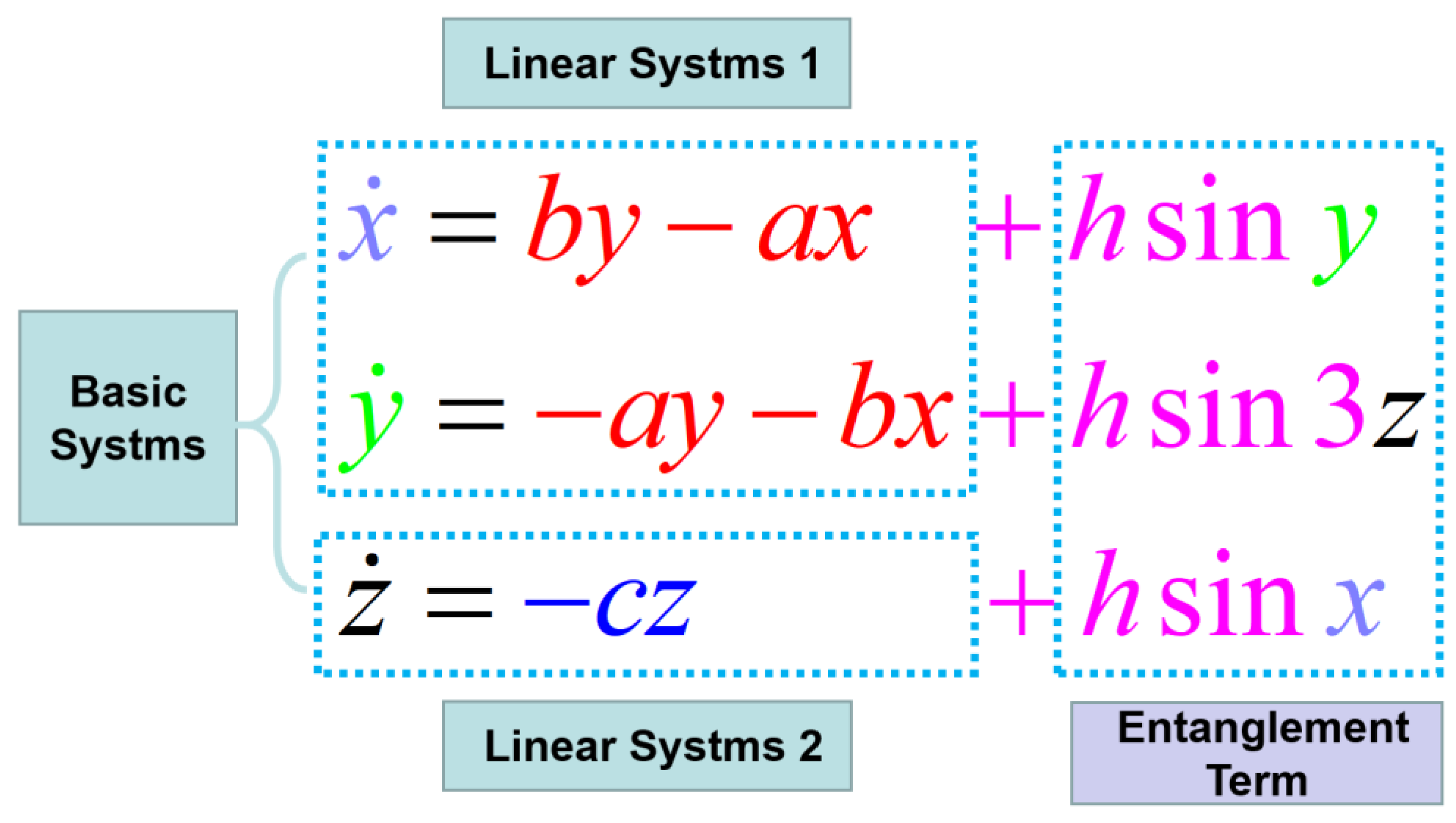
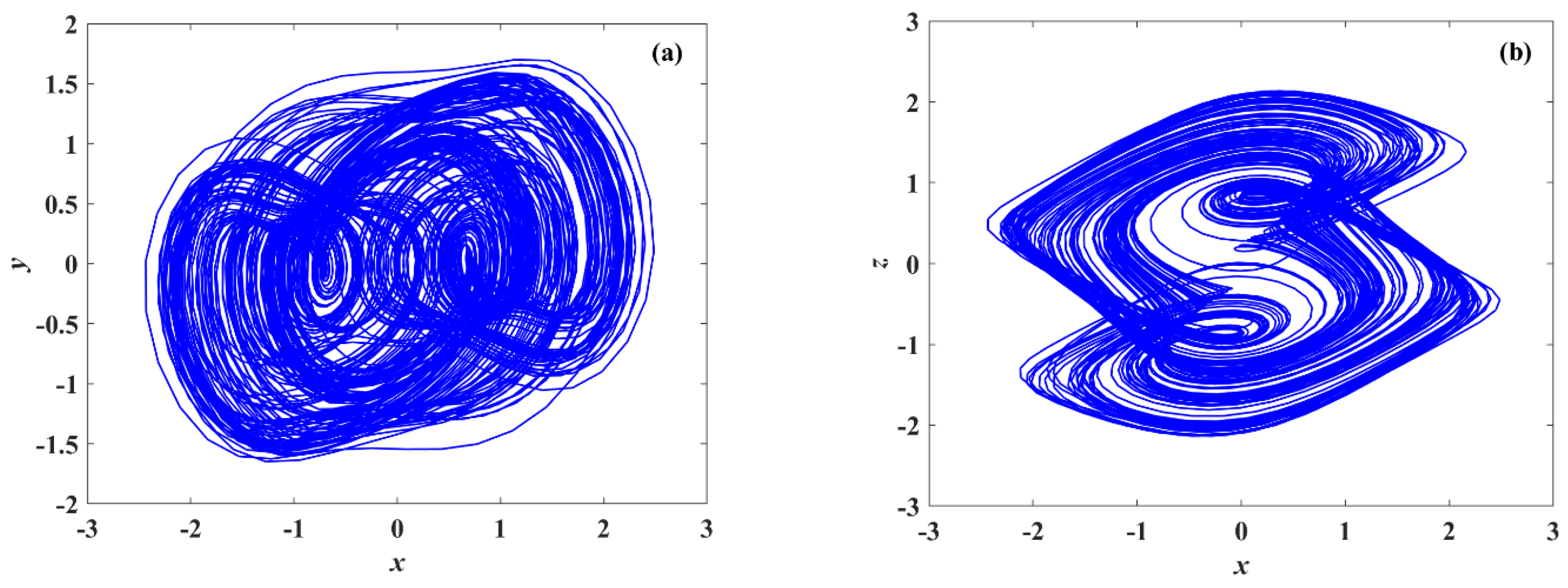
2. Description of Entanglement-Chaos System

A typical two-dimensional linear dynamic system model is:

$$\{\begin{array}{l}\dot{x}=by-ax\\ \dot{y}=-bx-ay\end{array}$$

(1)

In addition, a typical one-dimensional linear dynamic system model is:

$$\dot{z}=-cz$$

(2)

If the above two systems, namely System (1) and System (2), are entangled, a kind of entanglement dynamics system model can be obtained. The dynamic model equation is as follows:

$$\{\begin{array}{l}\dot{x}=by-ax+h\sin y\\ \dot{y}=-ay-bx+h\sin 3z\\ \dot{z}=-cz+h\sin x\end{array}$$

(3)

where x, y, and z represent state variables, a, b, c, and h are system parameters, and sin3z, cosx, and siny are entangled terms as dynamic systems. The construction process of the entanglement-chaos system is shown in Figure 1.

Make the system parameters the same as those in [33], and use the ODE45 function in the MATLAB software to solve Equation (3); we obtain the numerical solution of the nonlinear System (3), and draw the attractor trajectory of System (3), as shown in Figure 1. Through the calculation, it is found that the three LEs of the entangled chaotic System (3) are LE₁ = 2.03, LE₂ = 0.00, LE₃ = −9.02. The LEs of System (3) accord with the principle of the 3D chaotic system LEs (+,0,−); System (3) is chaotic. It can be seen from the attractor trajectory diagram of the system in Figure 2 that the attractor of the system has symmetric characteristics.

Set a = 2, b = 10, c = 3, and h = 18, [x(0), y(0), z(0)], as the initial conditions of the state variables, the values of which are [x(0), 2,3], and set x(0) to change between −50 and 50 with a change step of x(0) of 0.1. The bifurcation diagram and LEs of System (3) are shown in Figure 3. It can be seen that the x(0) change has no effect on the system, that is there is no multistable phenomenon in System (3).

3. Analysis of Memristive Entanglement System

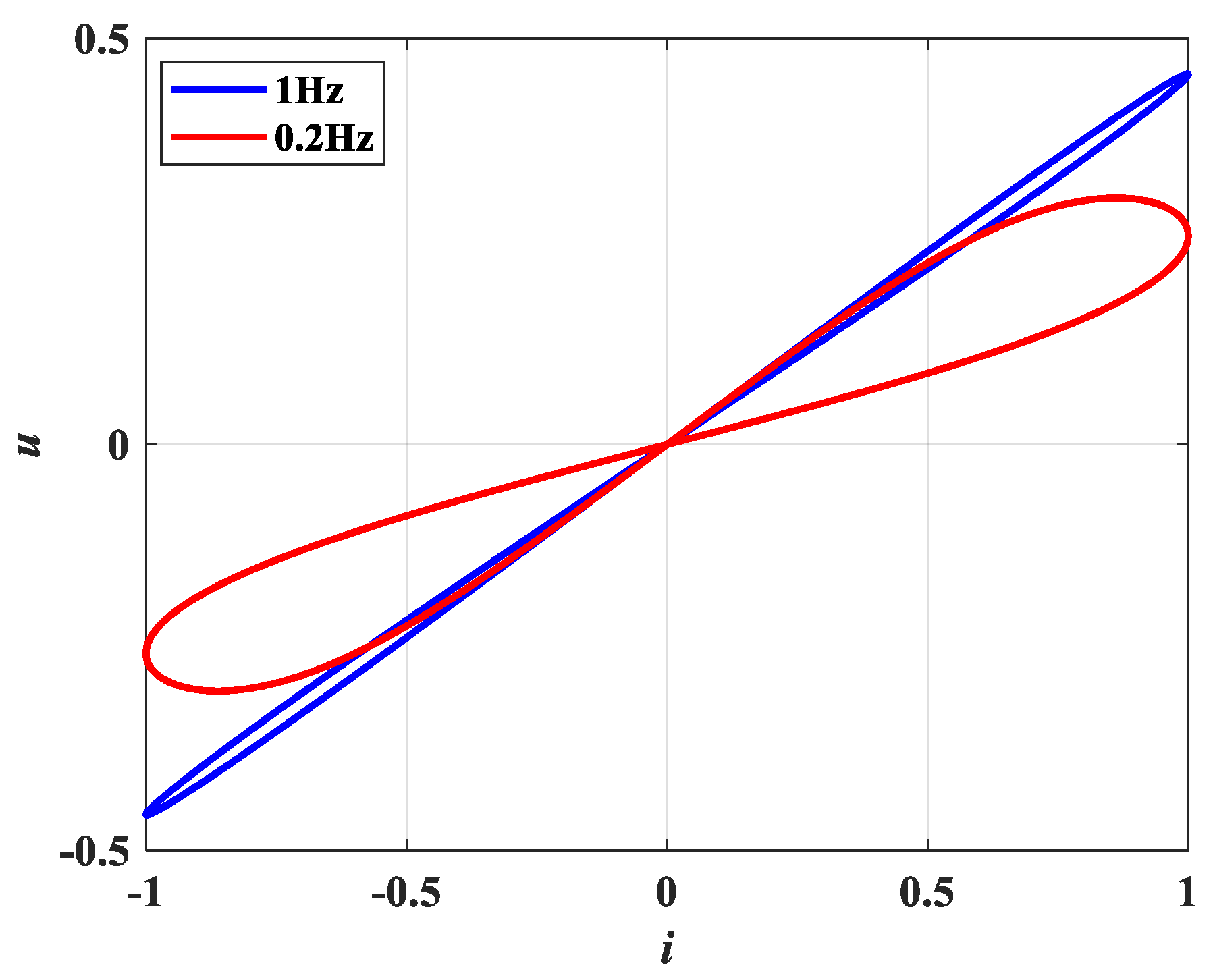
3.1. Memristive Entanglement System

A memristor is a passive two-terminal circuit element that describes the algebraic relationship between flux and charge [34]. There are two types of control, charge control (current control) and flux control (voltage control), and there are many models [35,36]. In this paper, the quadratic nonlinear flux control memristor is adopted, and its models are as follows:

$$\{\begin{array}{l}i=W\left(\varphi \right)u\\ W\left(\varphi \right)=\alpha +\beta {\varphi }^2\\ \dot{\varphi }=u\end{array}$$

(4)

where α and β are the parameters of the memristor model and are greater than 0. Figure 3 shows the voltage–current relationship of the memristor model with α = 2, β = 0.09 under a frequency f = 0.1 Hz and 1 Hz. It can be seen from Figure 4 that the current–voltage volt-ampere characteristic curve of the memristor is symmetrical.

W(φ) represents the voltage and current constraints in the memristor, which is a typical “8-like” hysteresis loop. The newly developed memristive system can be rewritten as:

$$\{\begin{array}{l}\dot{x}=by-ax+h\sin y+(\alpha +\beta w^2)y\\ \dot{y}=-ay-bx+h\sin 3z\\ \dot{z}=-cz+h\sin x\\ \dot{w}=y\end{array}$$

(5)

where x, y, z, and w are state variables, a, b, c, h, α, and β are system parameters, and 3z, cosx, and siny are entangled terms as dynamic systems. When a = 2, b = 10, c = 3, h = 18, α = 2, β = 0.09, and the initial condition [x(0), y(0), z(0), w(0)] = [0.1, 3, 2, w(0)], we use the ODE45 function in the MATLAB software to solve Equation (5) and obtain the numerical solution of the system, then we draw the phase trajectory of the system as shown in Figure 5. In Figure 5, the blue track indicates the initial value of the system to be (0.1, 3, 2, 5), and the red track indicates the initial value of the system to be (0.1, 3, 2, 6). From the system track phase diagram, it can be seen that the red attractor is periodic and the blue attractor is chaotic.

3.2. Dissipative Analysis

For the memristive chaotic System (5), its vector field divergence is:

$$\nabla V=\frac{\partial \dot{x}}{\partial x}+\frac{\partial \dot{y}}{\partial y}+\frac{\partial \dot{z}}{\partial z}+\frac{\partial \dot{w}}{\partial w}=-2a-c$$

(6)

Setting b = 13 and c = 1, when the control parameter a > 0, it is obviously negative, which means memristive chaotic systems are dissipative under a > 0.

3.3. Equilibrium Stability Analysis

To solve the equilibrium point of System (5), each equation of System (5) needs to be zero, that is:

$$\{\begin{array}{l}by-ax+h\sin y+(\alpha +\beta w^2)y=0\\ -ay-bx+h\sin 3z=0\\ -cz+h\sin x=0\\ y=0\end{array}$$

(7)

According to Equation (7), it is easy to obtain that the equilibrium point of System (5) is $A=\left\{\right(x,y,z,w\left)\right|x=y=z=0,w=e\}$ and e is constant. This shows that the memristive chaotic system has a linear equilibrium point. At this time, it is linearized at the equilibrium point, which corresponds to the Jacobian matrix J as follows:

$$\mathrm{J}=\left[\begin{array}{cccc}-a& b+h+\alpha +\beta e^2& 0& 0\\ -b& -a& 3h& 0\\ h& 0& -c& 0\\ 0& 1& 0& 0\end{array}\right]$$

(8)

The systems characteristic equation corresponding to matrix J can be written as:

$$P\left(\lambda \right)={\lambda }^4+c_1{\lambda }^3+c_2{\lambda }^2+c_3\lambda +c_4$$

(9)

where, c₁, c₂, c₃, and c₄ are the coefficients of the characteristic equation.

$$c_1=2a+c,c_2=a^2+2ac+b^2+b{e}^2\beta +bh+\alpha b$$

$$c_3=c{a}^2-3bh+c{b}^2+bc{e}^2\beta +cbh+\alpha cb-3\beta e^2{h}^2-3h^3-3a{h}^2{c}_4=0$$

According to the Routh criterion, the equilibrium point is stable when c₄ > 0. However, it is calculated that c₄ = 0 in Equation (11). Therefore, the equilibrium point is always unstable.

3.4. 0–1 Test

When the system equation is unknown or the system is a fractional system, the maximum Lyapunov exponent must be calculated from the time series after the phase space reconstruction of the system is completed according to the embedding theory [37]. Recently, Gottwald G.A. and Melbourne I. put forward a reliable and effective method to detect whether a system is chaotic [37], that is the 0–1 test. For a time series, we can define the following two real functions:

$$\{\begin{array}{l}p(n)={\displaystyle \sum _{i=1}^n\varphi \left(i\right)\cos \left(\theta \right(i\left)\right)}\\ s(n)={\displaystyle \sum _{i=1}^n\varphi \left(i\right)\sin \left(\theta \right(i\left)\right)}\end{array}$$

(10)

where $\theta (i)=i\omega +{\displaystyle \sum _{j=1}^i\varphi \left(j\right)}$, and we draw the trajectory in the p-s plane. In the p-s plane, if the bounded trajectory is periodic and if it is similar to the unbounded trajectory of Brownian motion, it indicates that the system is chaotic. This method is used to study the x sequence of memristive System (5). Its parameters are the same as those in Figure 3. The obtained p-s diagram is shown in Figure 6. Figure 6a is a bounded regular graph, then the system trajectory is periodic. Figure 6b shows a similar Brownian motion, so the system trajectory is chaotic.

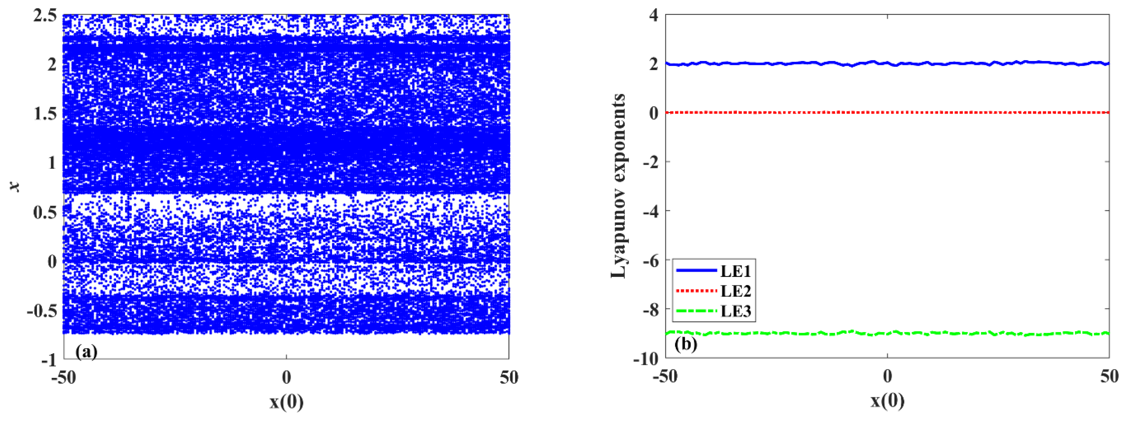
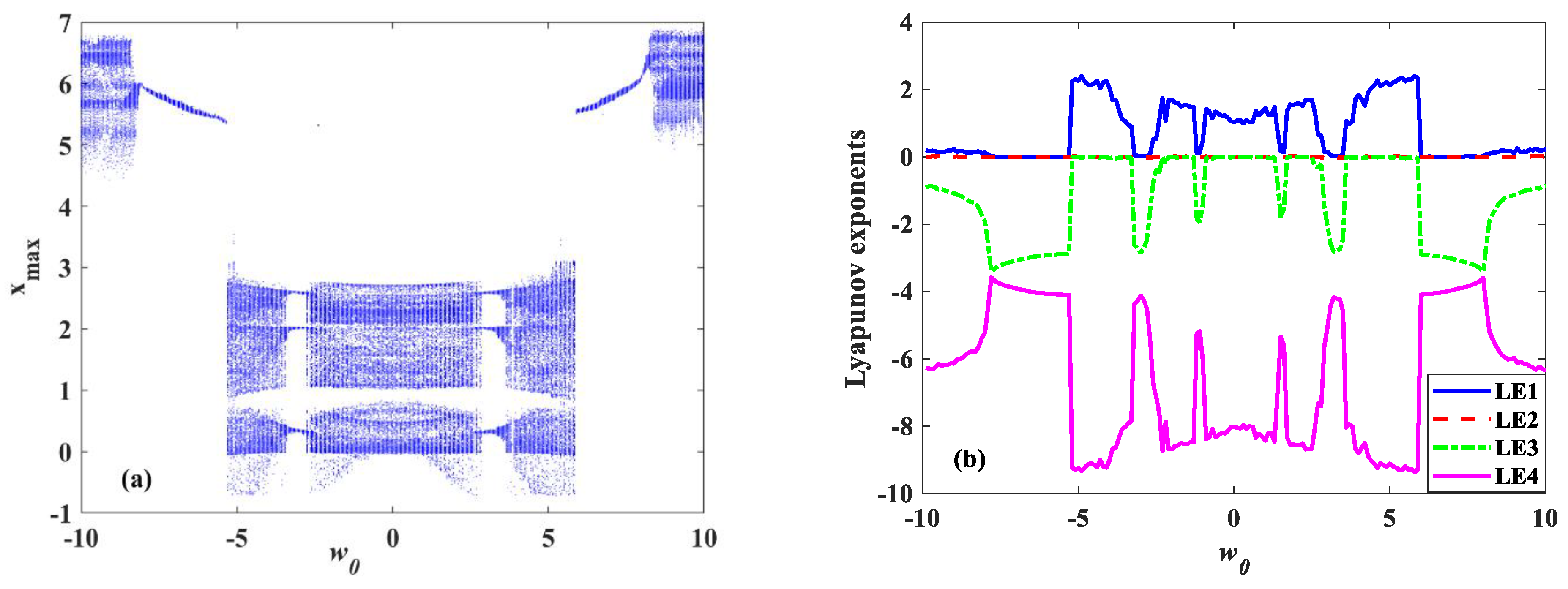
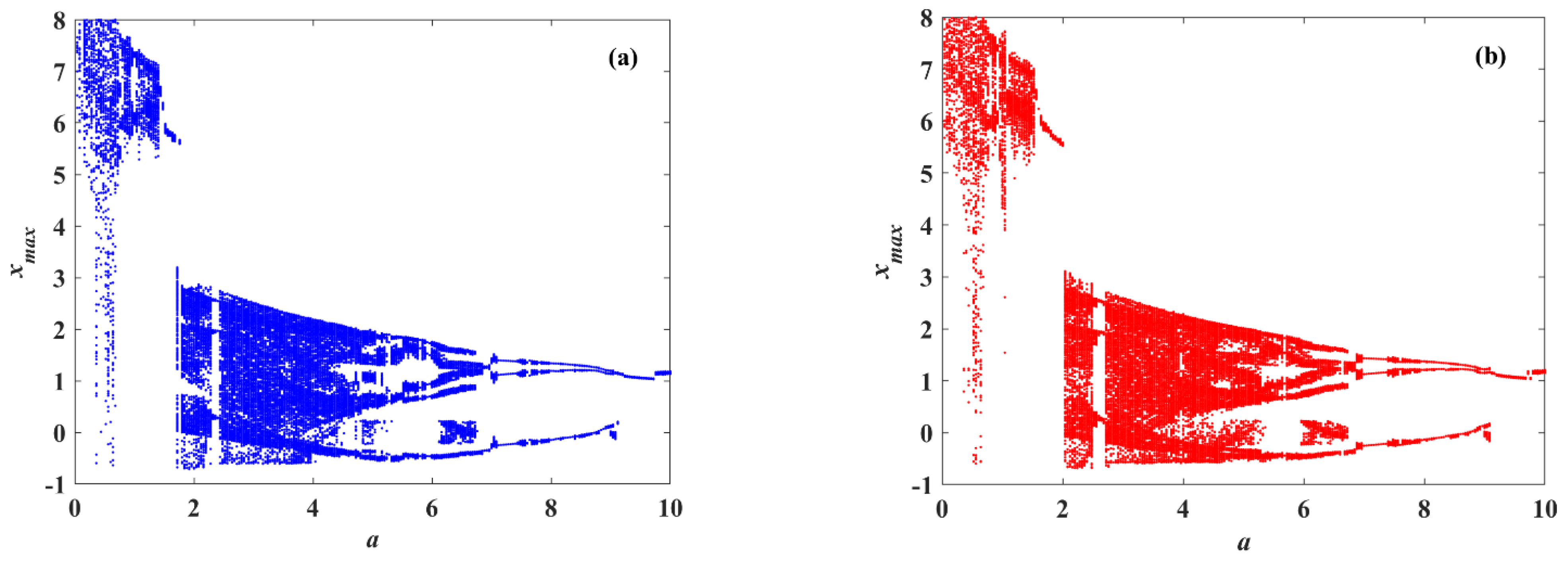
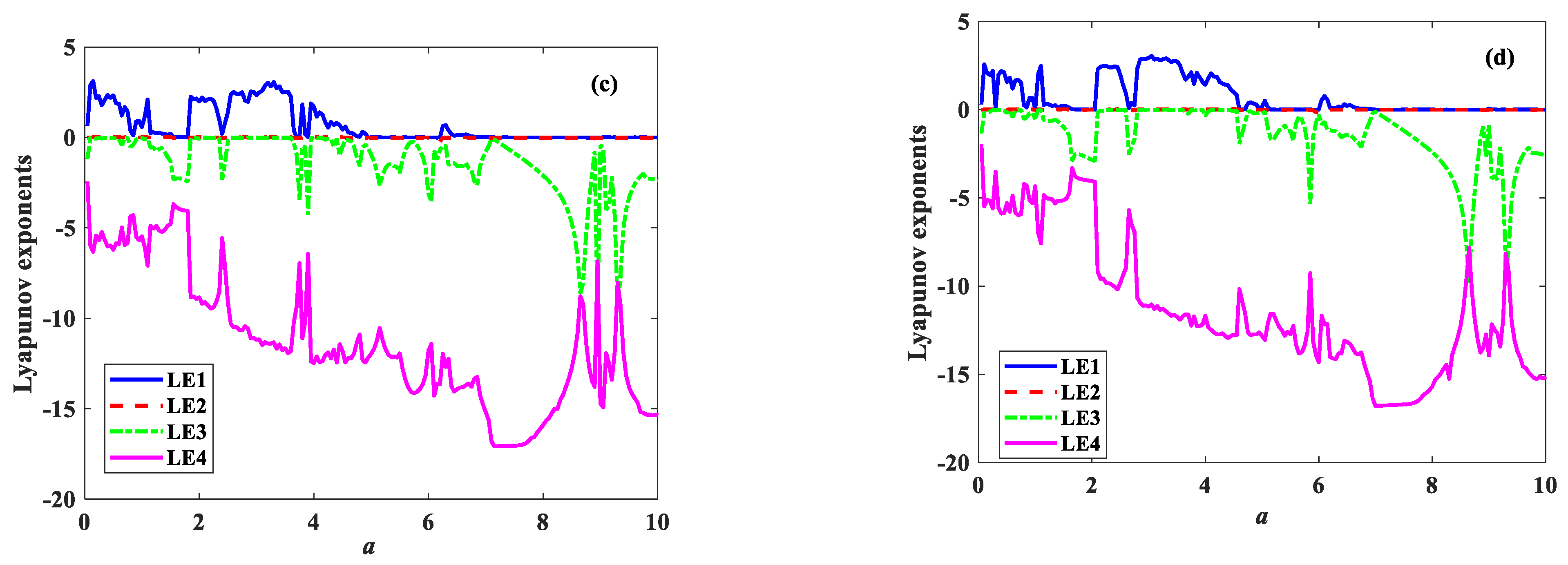
3.5. Multistability Analysis

The change of the system parameters will lead to different dynamic behaviors of a chaotic system. Choose them as variable parameters in turn, and analyze the dynamic characteristics of memristor System (3) by drawing the bifurcation diagram, LEs, and phase trajectory diagram. The numerical solution of System (5) is obtained by the Runge–Kutta method, and the bifurcation diagram is obtained by the maximum value of the system state variable x. For the computation of the LEs, we use the algorithm proposed by Wolf et al. [38].

First, x(0) is selected as the variable control parameter. Fix a = 2, b = 10, c = 3, h = 18, α = 2, and β = 0.09, x(0) from −100 to 100 with a step size of 1, and the initial values as [x(0), 3, 2, 5]. The bifurcation diagram is shown in Figure 7a, and its corresponding LE result is illustrated in Figure 6b. From Figure 7, It can be seen that, when the initial value changes, the nonlinear dynamic characteristics of the system are complex, with many coexisting attractors and multistable behaviors. When the parameter $x\left(0\right)\in [-100,-50]\cup [47,100]$, System (5) shows a periodic state. When $x\left(0\right)\in (-50,47)$, System (5) is in a chaos state and a periodic state appears alternately. When System (5) is in a periodic state, the LEs are equal to 0. When System (4) is in a chaotic state, the largest LEs are positive, as shown in Figure 7b.

Especially when $x\left(0\right)=-100$ and $x\left(0\right)=100$, System (5) presents two chaos states, and its coexisting attractors are shown in Figure 8a. When $x\left(0\right)=8$ and $x\left(0\right)=10$, the system is in a chaos and a periodic state, and its coexisting attractors are shown in Figure 8b.

Fixing the parameters a = 2, b = 10, c = 3, h = 18, α = 2, and β = 0.09, w(0) from −100 to 100 with a step size of 1, and the initial values set as [0.1, 3, 2, w(0)], the bifurcation diagram is shown in Figure 9a, and its corresponding LE result is illustrated in Figure 9b. From Figure 9, we can see that the system has complex chaotic characteristics, and the phenomenon of coexisting attractors appears. When parameter $w_0\in [-100,-60]\cup [60,100]$, System (5) shows a periodic state. When $w_0\in (-60,60)$, System (5) is in a chaotic state, and a periodic state appears alternately. When System (5) is in a periodic state, the maximum LE is 0. When System (5) is in a chaotic state, the largest LEs are positive, as shown in Figure 9b.

When $w\left(0\right)=-100$ and $w\left(0\right)=100$, System (5) presents e as a chaotic and periodic state, its coexisting attractor is shown in Figure 10a. When $w\left(0\right)=2$ and $w\left(0\right)=50$, the system is in a chaotic state, and its coexisting attractor is shown in Figure 10b. When $w\left(0\right)=75$ and $w\left(0\right)=2$, System (5) presents e as a chaotic and periodic state, and its coexisting attractor is shown in Figure 10c.

Fixing the parameters a = 2, b = 10, c = 3, h = 18, α = 2, and β = 0.09, w(0) from −10 to 10 with a step size of 0.1, and the initial values [0.1, 3, 2, w(0)], the bifurcation diagram is shown in Figure 10a, and its corresponding LE result is illustrated in Figure 11b. From Figure 11, we can see that the system has complex chaotic characteristics, and the phenomenon of coexisting attractors appears. When the parameter $w_0\in [-8,-5.3]\cup [5.3,8]$, System (4) shows a periodic state. When System (5) is in a periodic state, the Lyapunov exponents are equal to 0. When System (4) is in a chaotic state, the largest LEs are positive, as shown in Figure 11b.

Fix the parameters b = 10, c = 3, h = 18, α = 2. and β = 0.04, and let the parameter a change in the range of [0, 10]. Figure 12 shows the bifurcation diagram and LEs of the system under two different initial conditions. The bifurcation diagram of the system with initial conditions of [0.1, 3, 2, 5] is shown in Figure 12a, and the bifurcation diagram of the system with initial conditions of [0.1, 3, 2, 6] is shown in Figure 12b. Figure 12c,d show the Lyapunov exponent spectrum. According to Figure 11, under two different initial values, with the decrease of parameter a, the system enters chaos through the period-doubling bifurcation road, and the bifurcation diagram is similar to the Les; however, the details are different. Obviously, in a ∈ [0, 2], the chaotic region of x (0) = 5 is larger than that of x(0) = 6.

4. Complexity Analysis of the System

4.1. Completeness Calculation

Complexity is a quantitative index to measure the degree to which chaotic systems generate sequences close to random sequences. The greater the complexity, the higher the security of the system under the response parameters. In practical applications, a chaotic system should be as complex as possible to ensure the anti-interference and anti-interception ability of the spread spectrum communication system and the anti-cracking ability of the encryption algorithm. At present, LEs and bifurcation diagrams are commonly used in the dynamic analysis of chaotic systems. These methods can qualitatively analyze the dynamic characteristics of the system, but cannot quantitatively reflect the complexity and randomness of chaotic sequences. Therefore, the SE and C0 complexity algorithm are used to analyze the complexity and randomness of the simplest fractional-order memristive chaotic system, so that the chaotic sequence with higher complexity can be selected when the system is applied to chaotic image encryption.

Spectral entropy (SE) [39] adopts the time series generated by the system, x, y, or z, one of which is subjected to a Fourier transform to obtain the corresponding spectral entropy value. The complexity of C0 [40] is that the time series of the chaotic system is decomposed into regular and irregular components, and the proportion of irregular components in the series is measured by the proportion. Sample entropy is an improvement of approximate entropy and a new complexity test method. Compared with approximate entropy, sample entropy has two advantages: the calculation of sample entropy (SampEn) does not depend on the data length; sample entropy has better consistency, that is the change of parameters M and R has the same influence on the sample entropy.

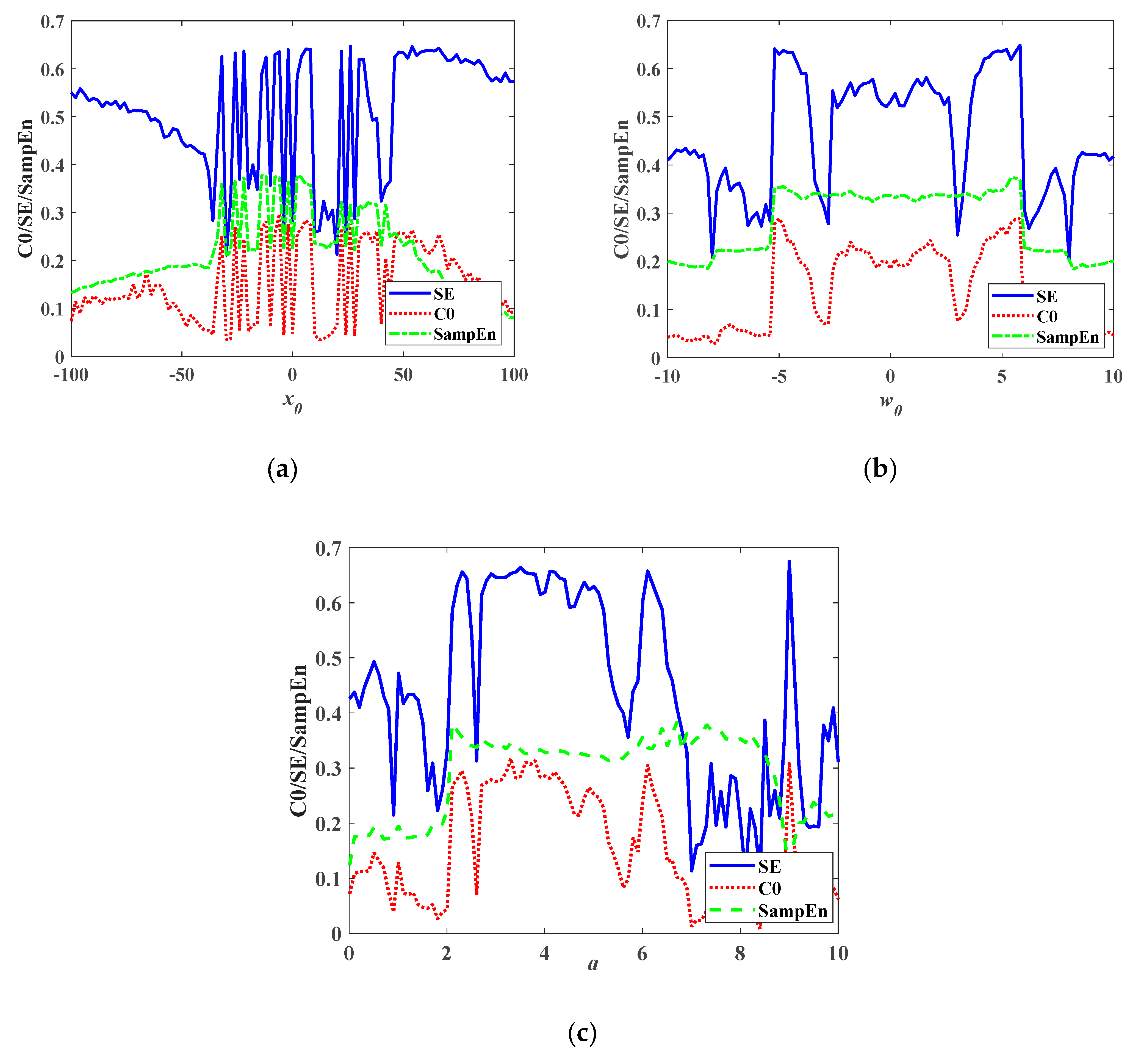
4.2. Complexity Analysis

We set the parameters a = 2, b = 10, c = 3, h = 18, α = 2, and β = 0.09, change x(0) from −100 to 100 with a step size of 0.5, and set the initial value of the system as [x(0), 3, 2, 5]. From Figure 13a, we can see that the complexity of the system under the change of x(0) is basically consistent with the change of the Lyapunov exponent in Figure 7b, which shows that the complexity can describe the influence characteristics of the parameters on the system.

We set parameters a = 2, b = 10, c = 3, h = 18, α = 2, and β = 0.09, set the initial value of the system as [0.1, 3, 2, w(0)], and let w(0) vary. The complexity of the system is shown in Figure 13b. The change of complexity is consistent with the change of the Lyapunov exponent in Figure 11b.

We set the parameters b = 10, c = 3, h = 18, α = 2, and β = 0.04, set the initial value of the system as [x(0), y(0), z(0), w(0)] = [0.1, 3, 2, 5], and let a vary. The complexity of the system is shown in Figure 13c. The change of complexity is consistent with the change of the Lyapunov exponent in Figure 12c.

The complexity of the system is consistent with the changing trend of the maximum Lyapunov exponent. In the chaotic state, the complexity remains basically the same, so it can be seen that the attractor result of the chaotic system does not become more complicated. Compared with the Lyapunov exponent calculation, the complexity calculation is faster, but there are some errors in the complexity. When the system is in a cycle, the SE complexity area is also larger.

4.3. C0 Complexity Diagram

The ordinate is the order w(0), and the abscissa is the system parameter x(0). The drawing method is as follows: divide the parameter and order plane into 101 × 101 points; calculate the C0 complexity of each point; express it in the form of a contour map. Compared with the parameter-fixed method to observe the system complexity, drawing chaotic maps requires more computation, but it can obtain more information about the system complexity and better grasp the system complexity from a macro perspective.

The C0 complexity diagram indicates the variation of the C0 complexity with initial condition [x(0), 3, 2, w(0)] and x(0) and w(0) changing, as shown in Figure 14. As can be seen from Figure 14, from the color bar on the right side of the figure, different colors represent complexity, that is the color ranges from blue to red and the complexity ranges from 0.05 to 0.3. A high-complexity area means that the system is chaotic or hyperchaotic, but the complexity diagram cannot show the details, such as the inability to distinguish periodic from chaotic.

5. Digital Implementation

There are two ways to realize a memristor nonlinear system, that is analog circuit and digital circuit technology. In this paper, the phase trajectory of the memristor system is mainly realized by a digital chip, and the digital chip is the STM32F103, while the A/D conversion chip is the TLV5618 12. Firstly, according to the voltage requirement of the digital chip, the memristor System (5) is discretized, and the discretization equation is as follows:

$$\{\begin{array}{l}x(n+1)=by(n)-ax(n)+h\sin y(n)+(\alpha +\beta w{\left(n\right)}^2)y(n)\\ y(n+1)=ay\left(n\right)-bx\left(n\right)+h\sin 3z\left(n\right)\\ z(n+1)=-cz\left(n\right)+h\sin x\left(n\right)\\ w(n+1)=y\left(n\right)\end{array}$$

(11)

According to the simulation process of MATLAB, in order to meet the requirements, set $\Delta$T = 0.001. The main control chip the STM32F103VE-EK is used in the system. The STM32F103VE-EK is a 32-bit single-chip microcomputer with a frequency as high as 72 MHz. It has two independent 12-bit A/D converter modules, which can output two signals at the same time. When a = 2, b = 10, c = 3, h = 18, α = 2, and β = 0.09, at the initial point [0.1, 3, 2, 5], the typical phase diagram of the chaotic system can be observed in the oscilloscope, as shown in Figure 15. When a = 2, b = 10, c = 3, h = 18, α = 2, and β = 0.09, at the initial point [0.1, 3, 2, 6], the typical phase diagram of the chaotic system can be observed in the oscilloscope, as shown in Figure 15. The numerical simulation of the output waveform of the oscilloscope and the system phase trajectory (as shown in Figure 5) in Figure 15 and Figure 16 is consistent (2).

6. Conclusions

Our objective was to further study the entanglement-chaos system with a memristor using standard nonlinear analysis tools such as LEs, bifurcation diagrams, C0/SE complexity, and phase diagrams. This showed that the system has a rich dynamic behavior, including coexistence attractors, multistability, and so on, and it is worth noting that different initial conditions have different coexistence attractors. Secondly, using the STM32F103VE-EK chip and the digital-to-analog converter, the phase diagram of the entanglement-chaos system with a memristor was displayed on the oscilloscope. This paper proved that the entanglement-chaos system with a memristor based on the STM32 can be applied to cryptography, memristive neural networks, artificial intelligence, and other related engineering fields.

References

1. Chua, L.O. Memristor—The missing circuit element. IEEE Trans. Circuit Theory 1971, 18, 507–519. [Google Scholar] [CrossRef]
2. Strukov, D.B.; Snider, G.S.; Stewart, D.R.; Williams, R.S. The missing memristor found. Nature 2008, 453, 80–83. [Google Scholar] [CrossRef] [PubMed]
3. Ebong, I.E.; Mazumder, P. CMOS and memristor-based neural network design for position detection. Proc. IEEE 2012, 100, 2050–2060. [Google Scholar] [CrossRef]
4. Yoon, J.H.; Wang, Z.; Kim, K.M.; Wu, H.; Ravichandran, V.; Xia, Q.; Hwang, C.S.; Yang, J.J. An artificial nociceptor based on a diffusive memristor. Nat. Commun. 2018, 9, 417. [Google Scholar] [CrossRef] [Green Version]
5. Itoh, M.; Chua, L.O. Memristor oscillators. Int. J. Bifurc. Chaos 2008, 18, 3183–3206. [Google Scholar] [CrossRef]
6. Bao, B.; Zhu, Y.; Ma, J.; Bao, H.; Wu, H.; Chen, M. Memristive neuron model with an adapting synapse and its hardware experiments. Sci. China Technol. Sci. 2021, 64, 1107–1117. [Google Scholar] [CrossRef]
7. Chen, M.; Li, M.; Yu, Q.; Bao, B.C.; Xu, Q.; Wang, J. Dynamics of self-excited attractors and hidden attractors in generalized memristor-based Chua’s circuit. Nonlinear Dyn. 2015, 81, 215–226. [Google Scholar] [CrossRef]
8. Yao, W.; Wang, C.; Sun, Y.; Zhou, C. Exponential multistability of memristive Cohen-Grossberg neural networks with stochastic parameter perturbations. Appl. Math. Comput. 2020, 386, 125483. [Google Scholar] [CrossRef]
9. He, S.; Sun, K.; Peng, Y.; Wang, L. Modeling of discrete fracmemristor and its application. AIP Adv. 2020, 10, 015332. [Google Scholar] [CrossRef]
10. Chen, M.; Sun, M.; Bao, H.; Hu, Y.; Bao, B. Flux-Charge Analysis of Two-Memristor-Based Chua’s Circuit: Dimensionality Decreasing Model for Detecting Extreme Multistability. IEEE Trans. Ind. Electron. 2019, 67, 2197–2206. [Google Scholar] [CrossRef]
11. Bao, B.C.; Hu, F.W.; Chen, M.; Xu, Q.; Yu, Y.J. Selfexcited and hidden attractors found simultaneously in a modified Chua’s circuit. Int. J. Bifurc. Chaos 2015, 25, 1550075. [Google Scholar] [CrossRef]
12. Chen, M.; Yu, J.; Bao, B.C. Finding hidden attractors in improved memristor-based Chua’s circuit. Electron. Lett. 2015, 51, 462–464. [Google Scholar] [CrossRef]
13. Leonov, G.A.; Kuznetsov, N.V.; Vagaitsev, V.I. Localization of hidden Chua’s attractors. Phys. Lett. A 2011, 375, 2230–2233. [Google Scholar] [CrossRef]
14. Zhang, X.; Li, C.; Chen, Y.; Herbert, H.C.I.U. A memristive chaotic oscillator with controllable amplitude and frequency. Chaos Solitons Fractals 2020, 139, 110000. [Google Scholar] [CrossRef]
15. Huang, L.; Zhang, X.; Zang, H.; Lei, T.; Fu, H. An Offset-Boostable Chaotic Oscillator with Broken Symmetry. Symmetry 2022, 14, 1903. [Google Scholar] [CrossRef]
16. Deng, Q.; Wang, C.; Yang, L. Four-Wing Hidden Attractors with One Stable Equilibrium Point. Int. J. Bifurc. Chaos 2020, 30, 2050086. [Google Scholar] [CrossRef]
17. Chen, M.; Wang, C.; Bao, H.; Ren, X.; Bao, B.C. Reconstitution for interpreting hidden dynamics with stable equilibrium point. Chaos Solitons Fractals 2020, 140, 110188. [Google Scholar] [CrossRef]
18. Kuznetsov, N.V.; Leonov, G.A. Hidden attractors in dynamical systems: Systems with no equilibria, multistability and coexisting attractors. IFAC Proc. Vol. 2014, 47, 5445–5454. [Google Scholar] [CrossRef] [Green Version]
19. Pham, V.-T.; Volos, C.; Jafari, S.; Kapitaniak, T. Coexistence of hidden chaotic attractors in a novel no-equilibrium system. Nonlinear Dyn. 2017, 87, 2001–2010. [Google Scholar] [CrossRef]
20. Zhang, S.; Zeng, Y. A simple Jerk-like system without equilibrium: Asymmetric coexisting hidden attractors, bursting oscillation and double full Feigenbaum remerging trees. Chaos Solitons Fractals 2019, 120, 25–40. [Google Scholar] [CrossRef]
21. Wei, Z.; Yousefpour, A.; Jahanshahi, H.; Kocamaz, U.E.; Moroz, I. Hopf bifurcation and synchronization of a five-dimensional self-exciting homopolar disc dynamo using a new fuzzy disturbance-observer-based terminal sliding mode control. J. Frankl. Inst. 2021, 358, 814–833. [Google Scholar] [CrossRef]
22. Peng, Y.; He, S.; Sun, K. A higher dimensional chaotic map with discrete memristor. AEU-Int. J. Electron. Commun. 2020, 129, 153539. [Google Scholar] [CrossRef]
23. Lai, Q.; Akgul, A.; Zhao, X.; Pei, H. Various types of coexisting attractors in a new 4D autonomous chaotic system. Int. J. Bifurc. Chaos 2017, 27, 1750142. [Google Scholar] [CrossRef]
24. Zhang, X.; Li, Z. Hidden extreme multistability in a novel 4D fractional-order chaotic system. Int. J. Non-Linear Mech. 2019, 111, 14–27. [Google Scholar] [CrossRef]
25. Zhang, S.; Zeng, Y.; Li, Z.; Wang, M.; Le, X. Generating one to four-wing hidden attractors in a novel 4D no-equilibrium chaotic system with extreme multistability. Chaos 2018, 28, 013113. [Google Scholar] [CrossRef] [PubMed]
26. Li, Q.; Zeng, H.; Li, J. Hyperchaos in a 4D memristive circuit with infinitely many stable equilibria. Nonlinear Dyn. 2015, 79, 2295–2308. [Google Scholar] [CrossRef]
27. Chen, H.; Lei, T.; Lu, S.; Dai, W.; Qiu, L.; Zhong, L. Dynamics and Complexity Analysis of Fractional-Order Chaotic Systems with Line Equilibrium Based on Adomian Decomposition. Complexity 2020, 2020, 5710765. [Google Scholar] [CrossRef]
28. Zhang, H.; Sun, K.; He, S. A fractional-order ship power system with extreme multistability. Nonlinear Dyn. 2021, 106, 1027–1040. [Google Scholar] [CrossRef]
29. Lu, Y.M.; Min, F.H. Dynamic analysis of symmetric behavior in flux-controlled memristor circuit based on field programmable gate array. Acta Phys. Sin. 2019, 68, 130502. [Google Scholar] [CrossRef]
30. Li, H.M.; Yang, Y.F.; Li, W.; He, S.B.; Li, C.L. Extremely rich dynamics in a memristor-based chaotic system. Eur. Phys. J. Plus 2020, 135, 579. [Google Scholar] [CrossRef]
31. Yuan, F.; Wang, G.; Wang, X. Extreme multistability in a memristor-based multi-scroll hyper-chaotic system. Chaos 2016, 26, 073107. [Google Scholar] [CrossRef] [PubMed]
32. Zhang, H.; Liu, X.; Shen, X.; Liu, J. Chaos entanglement: A new approach to generate chaos. Int. J. Bifurc. Chaos 2013, 23, 30014. [Google Scholar] [CrossRef]
33. Lei, T.; Mao, B.; Zhou, X.; Fu, H. Dynamics Analysis and Synchronous Control of Fractional-Order Entanglement Symmetrical Chaotic Systems. Symmetry 2021, 13, 1996. [Google Scholar] [CrossRef]
34. Ventra, M.D.; Pershin, Y.V.; Chua, L.O. Circuit elements with memory: Memristors, memcapacitors, and meminductors. Proc. IEEE 2009, 97, 1717–1724. [Google Scholar] [CrossRef] [Green Version]
35. Muthuswamy, B. Implementing memristor based chaotic circuits. Int. J. Bifurc. Chaos 2010, 20, 1335–1350. [Google Scholar] [CrossRef]
36. Iu, H.H.C.; Yu, D.S.; Fitch, A.L.; Sreeram, V.; Chen, H. Controlling Chaos in a Memristor Based Circuit Using a Twin-T Notch Filter. IEEE Trans. Circuits Syst. I Regul. Pap. 2011, 58, 1337–1344. [Google Scholar] [CrossRef]
37. Sun, K.H.; Liu, X.; Zhu, C.X. 0-1 test algorithm for chaos and its applications. Chin. Phys. B 2010, 19, 110510. [Google Scholar] [CrossRef]
38. Wolf, A.; Swift, J.B.; Swinney, H.L.; Vastano, J.A. Determining Lyapunov exponents from a time series. Physica 1985, 16, 285–317. [Google Scholar] [CrossRef]
39. Phillip, P.A.; Chiu, F.L.; Nick, S.J. Rapidly detecting disorder in rhythmic biological signals: A spectral entropy measure to identify cardiac arrhythmias. Phys. Rev. E 2009, 79, 011915. [Google Scholar]
40. Shen, E.H.; Cai, Z.J.; Gu, F.J. Mathematical foundation of a new complexity measure. Appl. Math. Mech. 2005, 26, 1188–1196. [Google Scholar]
Figure 1. Block diagram of constructing the entanglement-chaos system.
Symmetry 14 02586 g001
Figure 2. Attractor trajectory diagrams of System (3). (a) xy phase diagram; (b) xz phase diagram.
Symmetry 14 02586 g002
Figure 3. Bifurcation diagram and LEs of System (3) with x ( 0 ) [ 50 , 50 ] . (a) Bifurcation diagram; (b) LEs.
Symmetry 14 02586 g003
Figure 4. Pinned hysteresis loop of the memristor with different frequencies.
Symmetry 14 02586 g004
Figure 5. System phase diagram trajectory in different projections of chaotic System (5) from initial values (0.1, 3, 2, 5) and (0.1, 3, 2, 6). (a) System phase diagram trajectory in the xy plane; (b) system phase diagram trajectory in the xz plane.
Symmetry 14 02586 g005
Figure 6. ps plane diagrams in different projections of memristive chaotic System (2). (a) Initial values (0.1, 3, 2, 6); (b) initial values (0.1, 3, 2, 5).
Symmetry 14 02586 g006
Figure 7. Bifurcation diagram and LEs of System (2) with initial condition [x0, y0, z0, w0] = [x(0), 3, 2, 5]. (a) Bifurcation diagram; (b) LEs.
Symmetry 14 02586 g007
Figure 8. Various coexisting attractors with different values. (a) x(0) = −100 and x(0) = 100; (b) x(0) = 8 and x(0) = 10.
Symmetry 14 02586 g008
Figure 9. Bifurcation diagram and LEs of System (2) with initial condition [x0, y0, z0, w0] = [0.1, 3, 2, w(0) [−100, 100]]. (a) Bifurcation diagram; (b) LEs.
Symmetry 14 02586 g009
Figure 10. Various coexisting attractors with different values: (a) w ( 0 ) = 100 and w ( 0 ) = 100 ; (b) w ( 0 ) = 8 and w ( 0 ) = 10 ; (c) w ( 0 ) = 2 and w ( 0 ) = 75 .
Symmetry 14 02586 g010
Figure 11. Bifurcation diagram and LEs of System (5) with initial condition [x0, y0, z0, w0] = [0.1, 3, 2, w(0) [−10,10]]. (a) Bifurcation diagram; (b) Les.
Symmetry 14 02586 g011
Figure 12. Bifurcation and LEs of the system with a varying in [0, 10]. (a) Bifurcation of the system with [x(0), y(0), z(0), w(0)] = [0.1, 3, 2, 5]; (b) bifurcation of the system with [x(0), y(0), z(0), w(0)] = [0.1, 3, 2, 6]; (c) LEs of the system with [x(0), y(0), z(0), w(0)] = [0.1, 3, 2, 5]; (d) LEs of the system with [x(0), y(0), z(0), w(0)] = [0.1, 3, 2, 6].
Symmetry 14 02586 g012aSymmetry 14 02586 g012b
Figure 13. Complexity of the system with the parameters varying. (a) x0 varying; (b) w0 varying; (c) a varying.
Symmetry 14 02586 g013
Figure 14. C0 complexity in the w(0)−x(0) plane.
Symmetry 14 02586 g014
Figure 15. Oscilloscope display phase diagram of System (13) from initial values (0.1, 3, 2, 5). (a) Phase portraits in the x-y plane; (b) phase portraits in the x-z plane.
Symmetry 14 02586 g015
Figure 16. Oscilloscope display phase diagram of systems (13) from initial values (0.1, 3, 2, 6). (a) Phase portraits in the x-y plane; (b) phase portraits in the x-z plane.
Symmetry 14 02586 g016
Publisher’s Note: MDPI stays neutral with regard to jurisdictional claims in published maps and institutional affiliations.