
The g-Good-Neighbor Conditional Diagnosability of Exchanged Crossed Cube under the MM* Model
 ,
,
Abstract
1. Introduction
2. Preliminaries
2.1. Notations
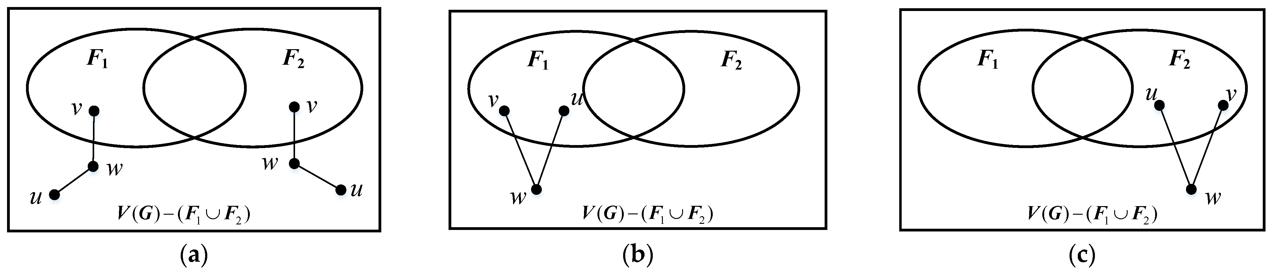
2.2. The MM* Model
2.3. Connectivity and Diagnosability
- There are two vertices and there is a vertex such that and ;
- There are two vertices and there is a vertex such that and ;
- There are two vertices and there is a vertex such that and ;

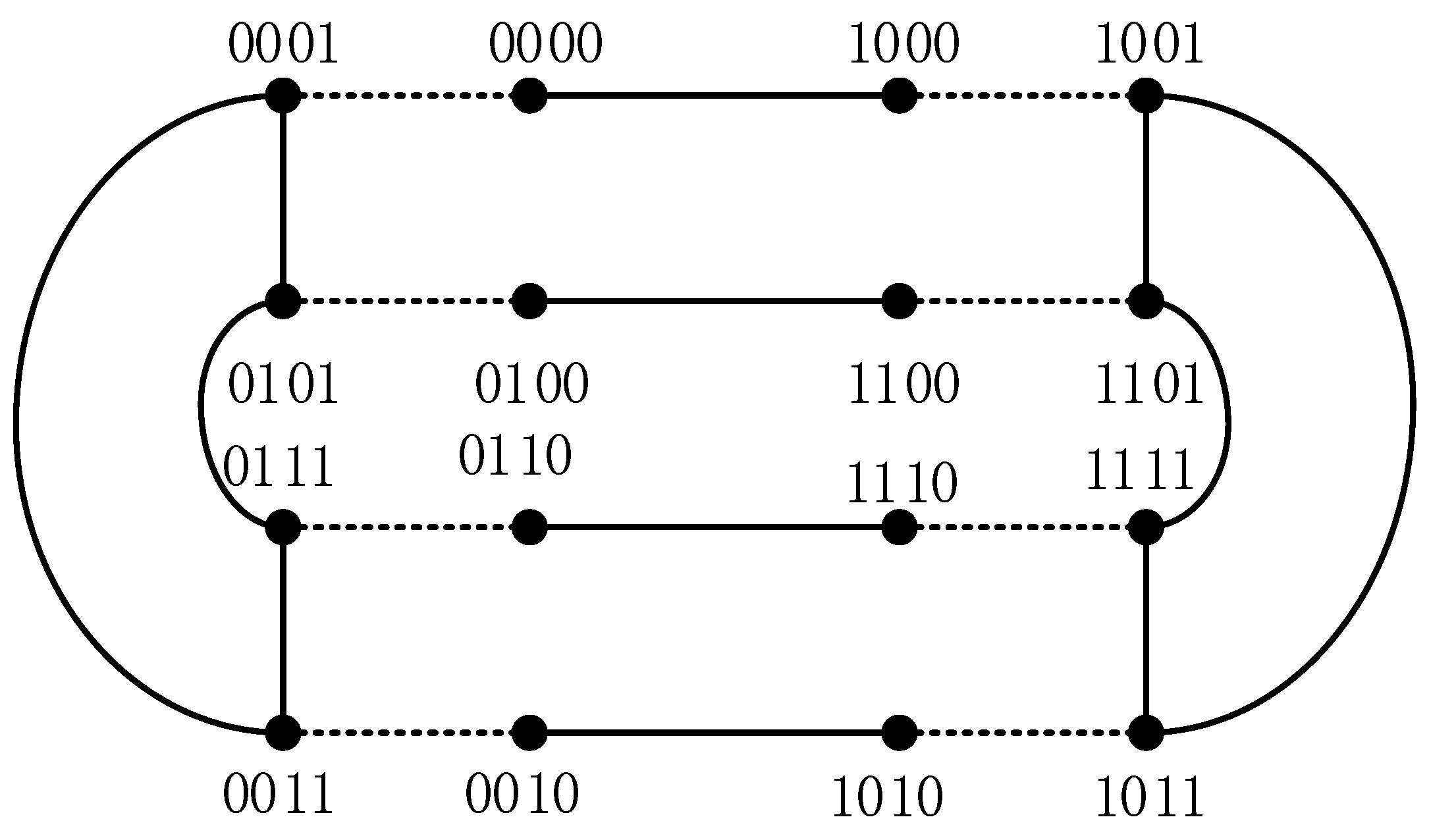
2.4. The Exchanged Crossed Cube
- : implies that , ;
- : implies that , , there exists an integer () such that , ; if is even, , , where ;
- : implies that , , there exists an integer () such that , ; if is even, , , where .
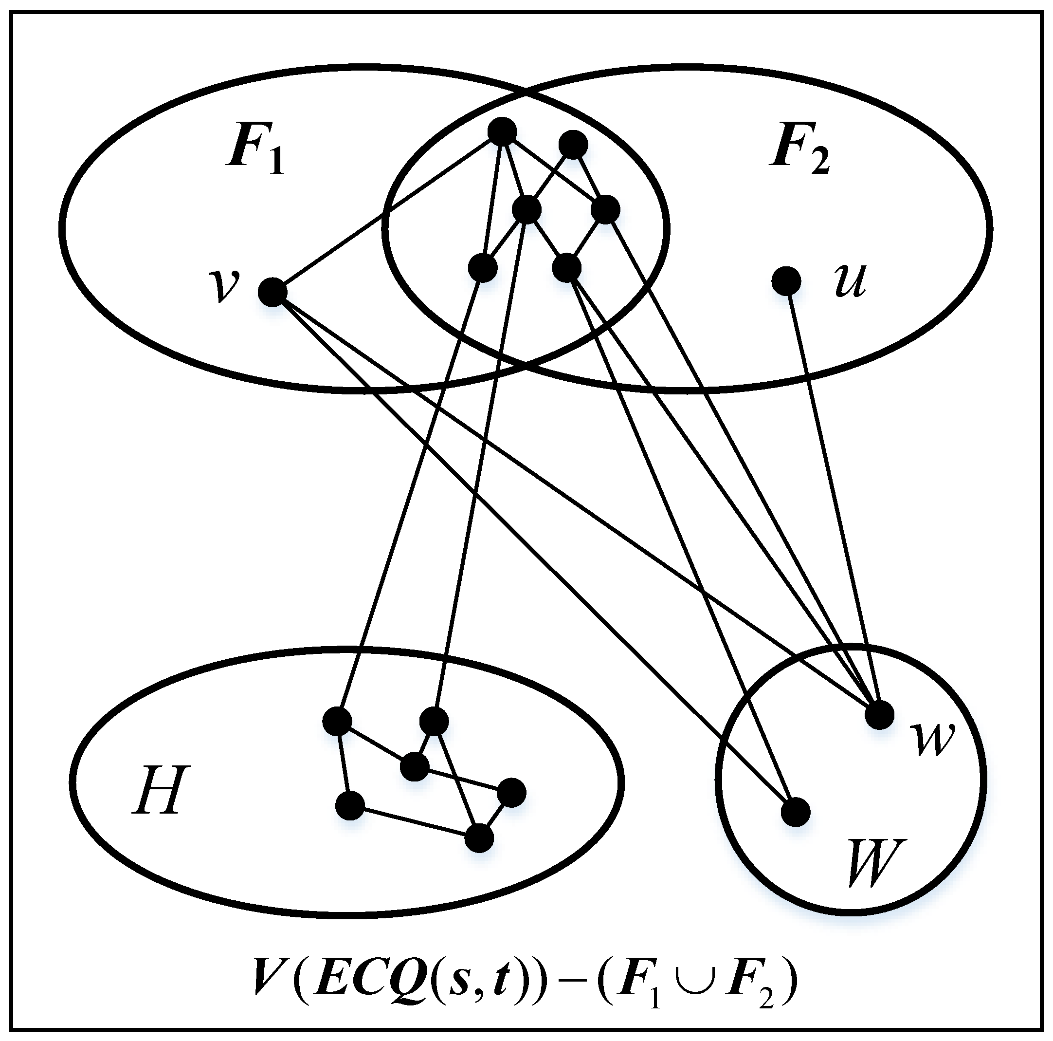
3. The g-Good-Neighbor Conditional Diagnosability of ECQ(s,t) under the MM* Model
- Case 1:
- Case 2:
- Case 3:
- Case 1. .
- Subcase 1.1. .
- Subcase 1.2. .
- Case 2. .
- Case 3. .
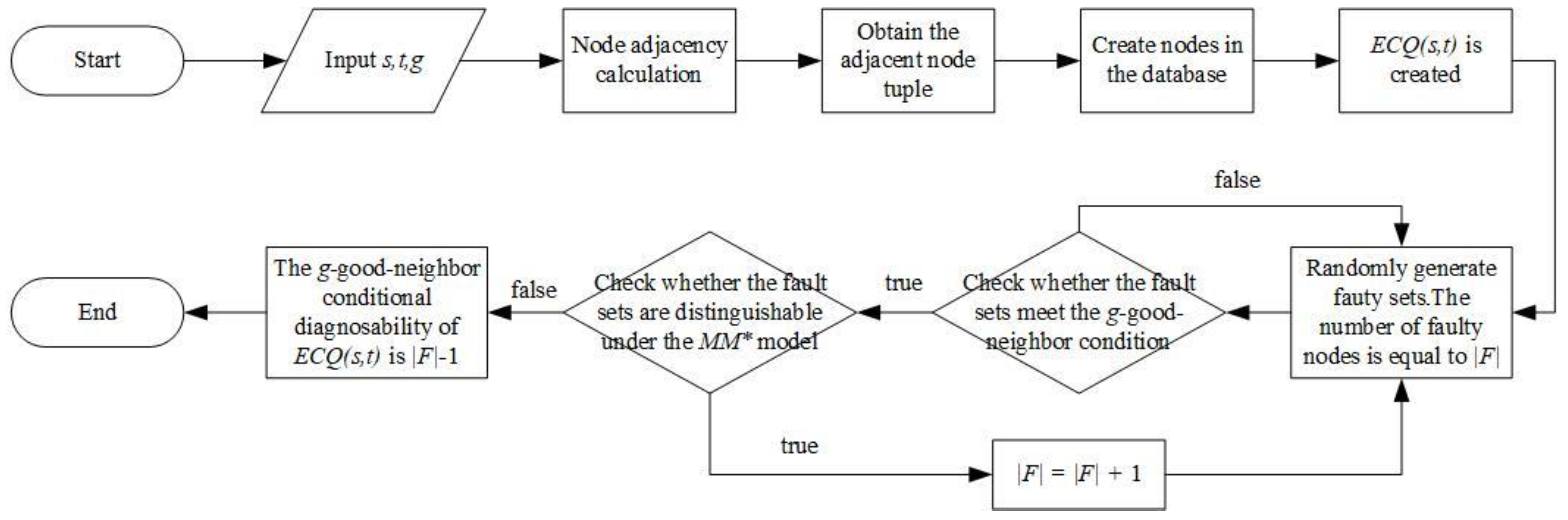
4. Simulation Experiment and Analysis
- STEP 1: Construct the network structure.
- STEP 2: Random generate g-good-neighbor conditional fault sets (k = 1, 2).
| Algorithm 1: Generate g-good-neighbor fault sets |
| Input:g, |F|, nodes, tuples |
| Output:g-good-neighbor fault sets F1, F2 |
| 1 nodeMap = {}; |
| 2 F1 = {}; |
| 3 F2 = {}; |
| 4 for node ∈ nodes |
| 5 nodeMap = Map(node, CountNeighbor (FindNeighber (node)) |
| 6 end for |
| 7 for node ∈ nodes |
| 8 (F1, F2) = SelectRandomNodes(nodes, |F|) |
| 9 if node ∉ F1 OR node ∉ F2 |
| 10 if nodeMap(node) <g |
| 11 then |
| 12 continue |
| 13 else |
| 14 return (F1, F2) |
| 15 end if |
| 16 end if |
| 17 end for |
- STEP 3: check the distinguishability of fault sets.
| Algorithm 2: Distinguishable verification algorithm |
| Input:F1, F2 |
| Output: Distinguishable verification result of F1 and F2 |
| 1 for node ∈ F1 ∈ F2 |
| 2 NeighborNode = FindNeighbor (node) |
| 3 AllNeighborNode = addNeighborNode (NeighborNode) |
| 4 end for |
| 5 MaxFrequency = Max (CountFrequency (AllNeighborNode)) |
| 6 if MaxFrequency ≥ 2 |
| 7 return distinguishable = true |
| 8 else |
| 9 return distinguishable = false |
| 10 end if |
5. Conclusions
Author Contributions
Funding
Institutional Review Board Statement
Informed Consent Statement
Data Availability Statement
Acknowledgments
Conflicts of Interest
References
- TOP500. ORNL’s Frontier First to Break the Exaflop Ceiling. Available online: https://www.top500.org/lists/top500/2022/06/ (accessed on 20 August 2022).
- Preparata, F.P.; Metze, G.; Chien, R.T. On the connection assignment problem of diagnosable systems. IEEE Trans. Electron. Comput. 1967, EC-16, 848–854. [Google Scholar] [CrossRef]
- Malek, M. A comparison connection assignment for diagnosis of multiprocessor systems. In Proceedings of the 7th Annual Symposium on Computer Architecture, La Baule, France, 6–8 May 1980; pp. 31–36. [Google Scholar]
- Maeng, J.; Malek, M. A comparison connection assignment for self-diagnosis of multiprocesso rsystems. In Proceedings of the 11th International Symposium on Fault-Tolerant Computing, Portland, OR, USA, 24–26 June 1981; pp. 173–175. [Google Scholar]
- Sengupta, A.; Dahbura, A.T. On self-diagnosable multiprocessor systems: Diagnosis by the comparison approach. IEEE Trans. Comput. 1992, 41, 1386–1396. [Google Scholar] [CrossRef]
- Wang, S.; Ma, X. Diagnosability of arrangement graphs with missing edges under the MM* model. Int. J. Parallel Emergent Distrib. Syst. 2020, 35, 69–80. [Google Scholar] [CrossRef]
- Zhu, Q.; Li, L.; Liu, S.; Zhang, X. Hybrid fault diagnosis capability analysis of hypercubes under the PMC model and MM* model. Theor. Comput. Sci. 2019, 758, 1–8. [Google Scholar] [CrossRef]
- Guo, J.; Li, D.; Lu, M. The g-good-neighbor conditional diagnosability of the crossed cubes under the PMC and MM* model. Theor. Comput. Sci. 2019, 755, 81–88. [Google Scholar] [CrossRef]
- Wang, S.; Ren, Y. The 2-extra diagnosability of alternating group graphs under the PMC model and MM* model. Am. J. Comput. Math. 2018, 8, 42–54. [Google Scholar] [CrossRef]
- Wang, S.; Ren, Y. g-Good-neighbor diagnosability of arrangement graphs under the PMC model and MM* model. Information 2018, 9, 275. [Google Scholar] [CrossRef]
- Liu, H.; Hu, X.; Gao, S. The g-good neighbor conditional diagnosability of twisted hypercubes under the PMC and MM* model. Appl. Math. Comput. 2018, 332, 484–492. [Google Scholar] [CrossRef]
- Guo, C.; Leng, M.; Xiao, Z.; Peng, S. Conditional Diagnosability of Exchanged Hypercube Under the MM* Model. IEEE Access 2018, 6, 61151–61162. [Google Scholar] [CrossRef]
- Wang, S.; Wang, Z.; Wang, M.; Han, W. g-Good-neighbor conditional diagnosability of star graph networks under PMC model and MM* model. Front. Math. China 2017, 12, 1221–1234. [Google Scholar] [CrossRef]
- Wang, S.; Han, W. The g-good-neighbor conditional diagnosability of n-dimensional hypercubes under the MM⁎ model. Inf. Process. Lett. 2016, 116, 574–577. [Google Scholar] [CrossRef]
- Yuan, J.; Qiao, H.; Liu, A. The Rg-conditional diagnosability of international networks. Theor. Comput. Sci. 2022, 898, 30–43. [Google Scholar] [CrossRef]
- Li, L.; Zhang, X.; Zhu, Q.; Bai, Y. The 3-extra conditional diagnosability of balanced hypercubes under MM∗ model. Discret. Appl. Math. 2022, 309, 310–316. [Google Scholar] [CrossRef]
- Lai, P.-L.; Tan, J.J.; Chang, C.-P.; Hsu, L.-H. Conditional diagnosability measures for large multiprocessor systems. IEEE Trans. Comput. 2005, 54, 165–175. [Google Scholar]
- Hsu, G.-H.; Chiang, C.-F.; Shih, L.-M.; Hsu, L.-H.; Tan, J.J. Conditional diagnosability of hypercubes under the comparison diagnosis model. J. Syst. Archit. 2009, 55, 140–146. [Google Scholar] [CrossRef]
- Chang, N.-W.; Hsieh, S.-Y. Conditional Diagnosability of (n, k)-Star Graphs Under the PMC Model. IEEE Trans. Dependable Secur. Comput. 2016, 15, 207–216. [Google Scholar] [CrossRef]
- Guo, C.; Lemg, M.; Peng, S.; Wang, B. Conditional diagnosability of exchanged crossed cube under the MM model. J. Commun. 2017, 38, 106–124. [Google Scholar]
- Zhu, Q.; Liu, S.-Y.; Xu, M. On conditional diagnosability of the folded hypercubes. Inf. Sci. 2008, 178, 1069–1077. [Google Scholar] [CrossRef]
- Xu, M.; Thulasiraman, K.; Zhu, Q. Conditional diagnosability of a class of matching composition networks under the comparison model. Theor. Comput. Sci. 2017, 674, 43–52. [Google Scholar] [CrossRef]
- Chang, N.; Cheng, E.; Hsieh, S. Conditional diagnosability of Cayley graphs generated by transposition trees under the PMC model. ACM Trans. Des. Autom. Electron. Syst. (TODAES) 2015, 20, 1–16. [Google Scholar] [CrossRef]
- Peng, S.-L.; Lin, C.-K.; Tan, J.J.; Hsu, L.-H. The g-good-neighbor conditional diagnosability of hypercube under PMC model. Appl. Math. Comput. 2012, 218, 10406–10412. [Google Scholar] [CrossRef]
- Yuan, J.; Liu, A.; Ma, X.; Liu, X.; Qin, X.; Zhang, J. The g-Good-Neighbor Conditional Diagnosability of k-Ary n-Cubes under the PMC Model and MM* Model. IEEE Trans. Parallel Distrib. Syst. 2014, 26, 1165–1177. [Google Scholar] [CrossRef]
- Wei, Y.-L.; Xu, M. The g-good-neighbor conditional diagnosability of locally twisted cubes. J. Oper. Res. Soc. China 2018, 6, 333–347. [Google Scholar] [CrossRef]
- Ren, Y.; Wang, S. The g-good-neighbor diagnosability of locally twisted cubes. Theor. Comput. Sci. 2017, 697, 91–97. [Google Scholar] [CrossRef]
- Gu, M.-M.; Hao, R.-X.; Yu, A.-M. The 1-Good-Neighbor Conditional Diagnosability of Some Regular Graphs. J. Interconnect. Netw. 2017, 17, 1741001. [Google Scholar] [CrossRef]
- Wei, Y.; Xu, M. The 1,2-good-neighbor conditional diagnosabilities of regular graphs. Appl. Math. Comput. 2018, 334, 295–310. [Google Scholar]
- Wang, S.; Yang, Y. The 2-good-neighbor (2-extra) diagnosability of alternating group graph networks under the PMC model and MM* model. Appl. Math. Comput. 2017, 305, 241–250. [Google Scholar] [CrossRef]
- Lin, L.; Hsieh, S.-Y.; Chen, R.; Xu, L.; Lee, C.-W. The Relationship Between g-Restricted Connectivity and g-Good-Neighbor Fault Diagnosability of General Regular Networks. IEEE Trans. Reliab. 2018, 67, 285–296. [Google Scholar] [CrossRef]
- Cheng, D. A relationship between g-good-neighbour conditional diagnosability and g-good-neighbour connectivity in regular graphs. Int. J. Comput. Math. Comput. Syst. Theory 2018, 3, 47–52. [Google Scholar] [CrossRef]
- Cheng, E.; Qiu, K.; Shen, Z. A general approach to deriving the g-good-neighbor conditional diagnosability of interconnection networks. Theor. Comput. Sci. 2019, 757, 56–67. [Google Scholar] [CrossRef]
- Wang, S.; Wang, M. The g-good-neighbor and g-extra diagnosability of networks. Theor. Comput. Sci. 2019, 773, 107–114. [Google Scholar] [CrossRef]
- Li, K.; Mu, Y.; Li, K.; Min, G. Exchanged crossed cube: A novel interconnection network for parallel computation. IEEE Trans. Parallel Distrib. Syst. 2012, 24, 2211–2219. [Google Scholar] [CrossRef]
- Loh, P.K.; Hsu, W.-J.; Pan, Y. The exchanged hypercube. IEEE Trans. Parallel Distrib. Syst. 2005, 16, 866–874. [Google Scholar] [CrossRef]
- Efe, K. The crossed cube architecture for parallel computation. IEEE Trans. Parallel Distrib. Syst. 1992, 3, 513–524. [Google Scholar] [CrossRef]
- Ning, W. The super connectivity of exchanged crossed cube. Inf. Process. Lett. 2016, 116, 80–84. [Google Scholar] [CrossRef]
- Ning, W. The h-connectivity of exchanged crossed cube. Theor. Comput. Sci. 2017, 696, 65–68. [Google Scholar] [CrossRef]
- Ning, W.; Feng, X.; Wang, L. The connectivity of exchanged crossed cube. Inf. Process. Lett. 2015, 115, 394–396. [Google Scholar] [CrossRef]
- Guo, C.; Leng, M.; Wang, B. The conditional diagnosability of exchanged crossed cube. IEEE Access 2018, 6, 29994–30004. [Google Scholar] [CrossRef]
- Peng, S.; Luo, C.; Wang, B.; Xiao, Z. Research on g-Good-Neighbor Conditional Diagnosability of Exchanged Crossed Cube. Comput. Eng. Appl. 2019, 51–58, 92. [Google Scholar]
- Bondy, J.A.; Murty, U.S.R. Graph Theory; Springer: New York, NY, USA, 2010. [Google Scholar]
- Latifi, S.; Hegde, M.; Naraghi-Pour, M. Conditional connectivity measures for large multiprocessor systems. IEEE Trans. Comput. 1994, 43, 218–222. [Google Scholar] [CrossRef]


| Platform Attribute | Details |
|---|---|
| RAM | 8.0 G |
| CPU | Intel(R) Core(TM) i7-9750H CPU @2.60 GHz 32-core processor |
| GPU | NVIDIA GeForce GTX 1650 |
| Operating System | Windows 10 |
| Development tools | Python-3.8, neo4j-community-4.3.3, JDK11 |
| Runtime environment | python3, JDK 11 or above |
| Development languages | Python, Java, Cyper |
| Node Number | Edge Number | || | |||
|---|---|---|---|---|---|
| 2 | 2 | 32 | 48 | 1 | 5 |
| 2 | 3 | 64 | 112 | 1 | 5 |
| 2 | 4 | 128 | 256 | 1 | 5 |
| 2 | 5 | 256 | 576 | 1 | 5 |
| 3 | 3 | 128 | 256 | 1 | 7 |
| 3 | 3 | 128 | 256 | 2 | 11 |
| 3 | 4 | 256 | 576 | 1 | 7 |
| 3 | 4 | 256 | 576 | 2 | 11 |
| 3 | 5 | 512 | 1280 | 1 | 7 |
| 3 | 5 | 512 | 1280 | 2 | 11 |
| 4 | 4 | 512 | 1280 | 1 | 9 |
| 4 | 4 | 512 | 1280 | 2 | 15 |
| 4 | 4 | 512 | 1280 | 3 | 23 |
| 4 | 5 | 1024 | 2816 | 1 | 9 |
| 4 | 5 | 1024 | 2816 | 2 | 15 |
| 4 | 5 | 1024 | 2816 | 3 | 23 |
| 5 | 5 | 2048 | 6144 | 1 | 11 |
| 5 | 5 | 2048 | 6144 | 2 | 19 |
| 5 | 5 | 2048 | 6144 | 3 | 31 |
| 5 | 5 | 2048 | 6144 | 4 | 47 |
Publisher’s Note: MDPI stays neutral with regard to jurisdictional claims in published maps and institutional affiliations. |
© 2022 by the authors. Licensee MDPI, Basel, Switzerland. This article is an open access article distributed under the terms and conditions of the Creative Commons Attribution (CC BY) license (https://creativecommons.org/licenses/by/4.0/).
Share and Cite
Wang, X.; Li, H.; Sun, Q.; Guo, C.; Zhao, H.; Wu, X.; Wang, A. The g-Good-Neighbor Conditional Diagnosability of Exchanged Crossed Cube under the MM* Model. Symmetry 2022, 14, 2376. https://doi.org/10.3390/sym14112376
Wang X, Li H, Sun Q, Guo C, Zhao H, Wu X, Wang A. The g-Good-Neighbor Conditional Diagnosability of Exchanged Crossed Cube under the MM* Model. Symmetry. 2022; 14(11):2376. https://doi.org/10.3390/sym14112376
Chicago/Turabian StyleWang, Xinyang, Haozhe Li, Qiao Sun, Chen Guo, Hu Zhao, Xinyu Wu, and Anqi Wang. 2022. "The g-Good-Neighbor Conditional Diagnosability of Exchanged Crossed Cube under the MM* Model" Symmetry 14, no. 11: 2376. https://doi.org/10.3390/sym14112376
APA StyleWang, X., Li, H., Sun, Q., Guo, C., Zhao, H., Wu, X., & Wang, A. (2022). The g-Good-Neighbor Conditional Diagnosability of Exchanged Crossed Cube under the MM* Model. Symmetry, 14(11), 2376. https://doi.org/10.3390/sym14112376