1. Introduction
The large-scale application of online education gives more and more learners access to personalized E-learning materials. Many E-learning systems that provide unique learning experiences for each learner, such as [
1,
2,
3], have been proposed. Among these, the learning path personalization is an essential implementation towards the learner-oriented curriculum design [
4].
The learning path personalization methods can be categorized into two classes [
5]: Course Generation (CG) and Course Sequence (CS). The former generates a complete learning path for a learner, while the latter recursively generates a learning path based on the transactions of the learner during the learning process. Researchers have applied various techniques to create personalized learning paths through the years, such as recommendation systems, decision support systems, evolutionary algorithms (EA), data mining, artificial intelligence, etc.
Compared with the path planning for logistics [
6], robots [
7], and aircrafts [
8], which forms a sequence of temporal and spatial points, the learning path planning problem essentially picks up a sequence of learning materials that satisfy the learner’s needs. Take learning to bake as an example: suppose there is a content-rich database of baking knowledge, which may include texts, pictures, audios, videos, and even mini-games. The contents of these learning materials may relate to ingredients, equipment, and procedures. If someone with some basic baking skills wants to learn to bake cupcakes and has a very short amount of time to learn, then an appropriate learning path could be: (1) a list of ingredients for cupcakes; (2) ingredients for buttercream; (3) the procedures written in text. On the other hand, if someone with zero baking knowledge and has sufficient time to learn to be a baking master, then an appropriate learning path could be: (1) the nature of common ingredients demonstrated in both text and pictures; (2) serials of videos show how to operate commonly-used baking equipment, such as ovens, a chef’s machine, etc.; (3) a video tutorial of baking cupcakes, and the learning path can go on depending on his/her learning objectives. In any case, people with different needs and skill levels will be presented with different learning paths that best suit them.
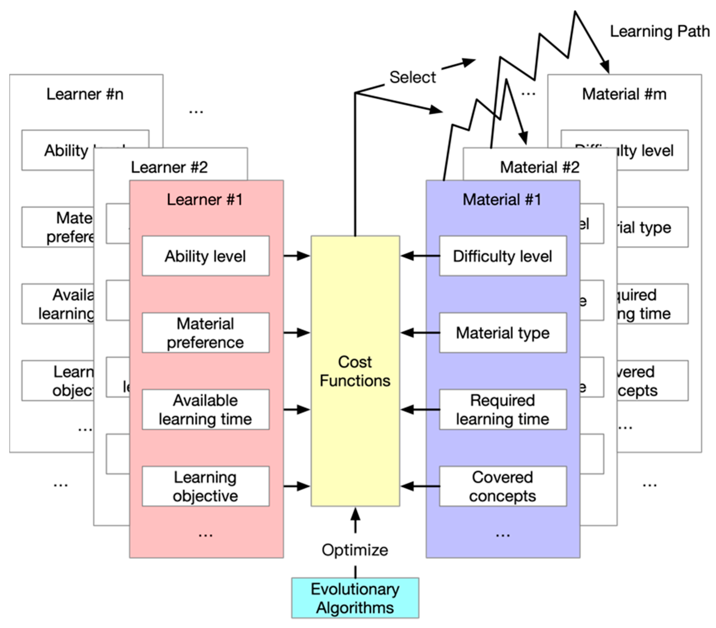
From the example mentioned above, we can find many attributes from both learners and learning materials. The EA approaches usually consider the learning path planning problem as an optimization problem that minimizes a cost function described by the attributes of the learner and generated learning path. The learner attributes may include profile, ability, preferences, goals, etc. The path attributes may include difficulty level, covered concepts, types, etc.
To better describe the relation between learner and learning material, symmetrical attribute pairs are often considered. For example, when the ability level of learner is assumed to affect the learning, the difficulty level of material should be included to match the learner; when the learning objective of learner affects the selection of materials, then the concepts covered by the material or the learning outcome of a material should be included as well.
Figure 1 depicts the symmetrical matching of the attributes derived from both learners and learning materials.
The learning path in the EA approaches is usually represented by binary strings [
9,
10,
11]. The issues of binary representation are two-fold: (1) binary representation is not capable of representing the sequence of materials in a path; (2) binary representation suffers severe scaling issues, which usually leads to poor performance when the problem scales up. On the other hand, integer representation can represent the material sequence [
12,
13], but the operators of the associated algorithm have to be carefully designed to deal with invalid solutions. Moreover, the algorithm-specific design of operators is challenging to implement into other algorithms, thus limiting the application.
Floating-point number representation, however, can represent any sequence by mapping the floating numbers to integers. The optimization problems associated with floating-number representation are generally referred to as continuous optimization problems. Usually, the algorithms for solving continuous optimization problems have the same scaling issue with the increasing number of variables. However, for a learning path planning problem, the length of the learning path is limited by the learner’s energy. Therefore, the scaling problem may be avoided by carefully designed path representation.
This research proposes a multi-attribute matching (MAM) model to describe the affinity between learner attributes and learning path attributes. The attributes of a learner include ability level, learning objective, learning style, and expected learning time. The attributes regarding the learning path include difficulty level, covered concepts, supported learning style, required learning time, and prerequisites. A set of affinity functions are proposed to represent several aspects of the MAM model. A variable-length continuous representation (VLCR) of a learning path is proposed to utilize the powerful search ability of continuous evolution algorithms and reduce the search space. An adaptive differential evolution algorithm based on [
14] is presented to optimize the MAM model and generate the learning path for a given learner.
The rest of the paper is organized as follows:
Section 2 reviews the related works,
Section 3 presents the formalized problem,
Section 4 introduces the VLCR and the improved differential evolution algorithm,
Section 5 evaluates the proposed system with problems of different scales, and
Section 6 concludes the paper.
2. Related Works
2.1. Learning Path Personalization
Technology development makes e-learning evolve to s-learning, i.e., smart learning [
15]. Personalized learning is considered an essential part of the smart learning environment, providing the learner with a customized learning plan that includes exercises, documents, videos, and audios. Learning path personalization offers a structure for organizing these learning materials, which concerns not only the contents to learn but the sequence of learning them.
The sequence of learning materials is constrained by the relation between the materials. The relation can be captured by a knowledge model, such as knowledge map [
16,
17], knowledge graph [
18,
19], or concept map [
20], etc. The model can either be built from the experts’ experience [
21] or via educational data mining technology [
22]. Many methods are explored to construct a learning path that satisfies the learner’s needs and the constraints of knowledge model. The representative methods include machine learning [
20,
23] and evolutionary algorithms [
24,
25]. In [
20], a set of learning paths are generated through a topological sorting algorithm and the long short-term memory neural network is trained to predict the learning effect of the learning path. In [
26], a learning path recommendation model is developed based on a knowledge graph. The learning paths that fit the learning objectives are generated at once, and the one with the highest score is recommended. Ref. [
27] gathered the learner creativity information via three creativity games, and the data mining technology of the decision tree is employed to generate a personalized learning path that optimizes the performance of creativity. Jugo [
28] developed a web-based system that analyzes the learning path pattern, recommends the learning path, and visualizes the learning path pattern.
The machine learning approach highly depends on existing learning patterns generated by topological algorithms or data mining technologies, which cannot make an effective recommendation for a new system (cold-start problem). More importantly, the machine learning approach focuses on the relations between materials rather than the relations between the learners and the materials. The recommended learning path largely depends on the statistics of past learning experiences and lacks consideration of the extensive needs of the learners.
2.2. Evolutionary Algorithms for Learning Path Generation
The evolutionary algorithm approach, on the other hand, considers the learning path generation as an optimization problem that seeks the optimal match between a learning path and the learner attributes. The most representative evolutionary algorithms include genetic algorithms (GA), ant colony optimization (ACO), particle swarm optimization (PSO), and differential evolution (DE) [
10]. Ref. [
12] applied the variable-length genetic algorithm to deal with the variable length in the learning path. Ref. [
13] applies an integer-encoded genetic algorithm to optimize the learning path of a Java course. The partially mapped crossover and the cycle crossover operators create offspring from parent solutions and prevent infeasible solutions. A discrete version of the hill-climbing algorithm is also used to create new solutions, and a simulated annealing mechanism is applied to select the solutions in the next generation. The combination of tournament selection with random initialization and cycle crossover is reported to have the highest solution quality. Ref. [
29] combines the GA and ACO to forge a collaborative optimization algorithm. The learning path is optimized based on the learning object, emotional state, cognitive ability, and learners’ performance. In [
25], the learning path of MOOC is recommended based on a multi-objective optimization model. Several learner criteria are considered, such as the number of enrollments, learning duration, and popularity. The model is solved by GA and ACO as well.
The learning path is essentially a sequence of learning materials; therefore, the learning path generation is a combinatorial optimization and NP-Hard problem [
30]. However, the evolutionary algorithms designed for such a problem require highly specialized operators to maintain the feasibility of the new solutions, such as the crossover operator in GA, the mutation operator in DE, and the velocity update in PSO. The continuous version of these evolutionary algorithms, however, guarantees the feasibility of a new solution given a suitable solution representation scheme. We will discuss a stream of high-efficiency continuous evolutionary algorithms, the differential evolution, in the following Subsection, and the solution representation in the continuous form in
Section 4.
2.3. Adaptive Differential Evolution for Continuous Problems
As a competitive evolutionary algorithm, DE was initially proposed by [
31] for continuous optimization problems and then applied to generate the learning path [
32]. DE optimizes the vectors of a floating-point number using the difference between randomly selected pairs of vectors. It is observed that the parameters of DE are problem-dependent. Therefore, research on parameter adaptation of DE [
33] have been proposed. In recent years, Q-learning, as a model-free reinforcement learning algorithm [
34,
35,
36], has been applied to adjust the DE parameters as well [
37].
In the field of adaptive DE, JADE [
38] proposed to control the parameter in a self-adaptive manner. To enhance the performance of JADE, SHADE [
39] was proposed to utilize a history-based parameter adaptation scheme. In order to gain the computation advantage in the CEC competition 2014, the L-SHADE algorithm [
40] adopted the Linear Population Size Reduction (LPSR) in SHADE.
In 2016, Ref. [
41] proposed the LSHADE-EpSin algorithm, which incorporated the Ensemble Sinusoidal Parameter Adaptation and became the joint winner in the competition of CEC 2016. One year later, Ref. [
14] proposed an improved algorithm, LSHADE-
cnEpSin, to tackle the problems with high correlation between variables. LSHADE-
cnEpSin became the second winner in the competition of CEC 2017 [
42].
Learning path generation is a complex combination problem that involves a large number of decision variables. When the problem scales up, the performance of many traditional algorithms may deteriorate drastically. Therefore, parameter adaptation and population reduction are of great importance in solving such problems. Furthermore, the conventional combination optimization algorithms require the delicate design of operators to avoid infeasible solutions. Therefore, a continuous solution representation that fits all continuous algorithms is also needed. To design a system with high scaling and generalization ability, the LSHADE-cnEpSin and floating-point number representation are adopted in this research to ensure the quality of generated learning path.
3. Problem Formulation
The problem of personalized learning path consists of four parts: learner attributes, material attributes, decision variables, and cost function. The learner attributes describe the factors of the learner that are relevant to the learning path. In contrast, the material attributes describe the characteristics of the learning material that are most relevant to the learner. Decision variables describe how the learning path is constructed from the learning materials, and the cost function represents the quality of the generated learning path.
3.1. Learner Attributes
A set that includes learners is defined, where is the attribute set for the -th learner.
represents the learning ability of the -th learner. The value is unified based on the difficulty level of the learning materials in the database. A learner who understands a material with a particular difficulty level is considered equal or greater ability level than the material.
represents the learning objectives of the -th learner. is the number of total learning objectives that are pre-determined by the nature of the learning materials. denotes that the learner has -th learning object, denotes not.
represents the degree of inclination of the
-th learner towards four learning styles proposed by Felder and Silverman [
43]: visual/verbal, sensing/intuitive, sequential/global, and active/reflective. The learning style is unified into
for computational simplicity. For example,
is a unified active/reflective learning style attribute, when
the learner inclines to reflective learning style,
the learner inclines to active learning style, and
represents neutral inclination.
denotes the upper and lower bound of the expected course duration of learner , where is the lower bound and is the upper bound, and .
A learner’s attributes may be determined by questionnaires, pre-tests, and the learner’s input. Specifically, the learning objectives and the upper and lower bounds of the expected learning time can be obtained from the learner’s input; the learning styles are determined by completing the questionnaire mentioned in [
43]; the learning ability can be estimated by the learner’s feedback on some materials without prerequisites.
3.2. Material Attributes
A set of learning materials is defined, where is the attribute set of the -th learning material.
denotes the difficulty level of the -th learning material. The difficulty level is closely related to the learner’s ability mentioned above and can be ascertained based on the learner’s past performance.
denotes the covered concepts of the -th learning material. The total number of concepts is the same as the number of learning objects . represents the material contains concept , while means the opposite. A material covers one concept at least and concepts at most.
represents the matching level of material to the four learning styles. A visual material, such as a picture or video, has a high match with the visual learning style, while the reading material has a high match with the verbal learning style. The intuitive learning style welcomes material presented with symbols and equations, and a sensing learner prefers facts and data. Sequential learners learn materials step by step, while the global learner likes the big picture of the course. Active learners prefer interactive learning scenarios and reflective learners are usually theorists.
is the required time to learn material , which can be ascertained by the learning history of the previous learners.
is the prerequisites of material , where represents that material requires concept as a prerequisite, while means the opposite. A material can have 0~ prerequisite (s).
A material’s attributes may be determined by the designer/provider of the material and the accumulated feedback of the learners. Specifically, the covered concepts and the prerequisites can be determined by the material’s designer/provider. The difficulty level and the matching level to learning styles can be initially designated by the designer/provider of the material and then gradually modified by the learner feedback. For example, the feedback on understanding/not understanding the material can be used to determine the difficulty level, and the feedback on liking/not liking the type of material can be used to determine the matching level to the learning styles.
3.3. Decision Variables
For learner
,
, the number of materials in the learning path, is determined by the following:
where
and
are the upper and lower bounds of the number of included materials, respectively. The decision variables are
, where
represents the material index to be chosen in the material database. The last decision variable,
, represents the actual length of the learning path. Therefore, the actual learning path is
.
3.4. Cost Function
Without loss of generality, the problem of recommending a learning path to learner
is formalized as the following optimization problem:
where
is a mapping function that maps the attributes of learner
, the attributes of each material, and the learning path to a scaler set:
. When the learning path optimization problem takes a minimization form, the mapping function
represents the degree of repulsion between the learner attributes and the learning path. The lower the mapped value is, the better the learner is matched to the learning path. To fully cover the relation between the leaner attributes and the learning path, different matchings should be considered, which include (1) learner ability and material difficulty, (2) learning objective and the covered concepts of the selected materials, (3) learning style and material type, (4) the sequence of the materials and their prerequisites, and (5) the expected learning time of the learner and the required learning time of the learning path. The matchings mentioned above can be formalized into five affinity functions
, whose relation with the main mapping function
is as follows:
where
is the weight of the affinity functions.
3.4.1. Learner Ability and Material Difficulty
The affinity function
describes the average difference between the learner’s ability level and the materials’ difficulty level, as defined as follows.
3.4.2. Learning Objectives and Covered Concepts of Material
The affinity function
describes the average difference between the learning objectives and the covered concepts of the materials.
where
is the average number of materials for a learning objective and is defined as follows.
And
is the number of covered concepts of the selected materials.
The affinity punishes two cases: (1) the learning objectives are not covered by the selected materials, and (2) the materials cover more concepts than the objectives. Meanwhile, the affinity function considers the balance of the materials for each learning objective. If the covered concepts of the selected materials are the same as the learning objectives, and the number of materials is the same for each objective, .
3.4.3. Learning Style and Material Type
The affinity function
describes the average difference between the learning style and the supported learning style of the materials.
3.4.4. Material and Its Prerequisites
The affinity function
describes the average difference between the concept coverage of the learned materials before the current material and the prerequisites of the current material.
where
represents the coverage of concept
of the materials that precede the current material
, which is defined as follows.
If the previous materials cover the prerequisite of the current material, returns zero, otherwise, one. Suppose the prerequisites of all the materials are satisfied by the previous materials, .
3.4.5. The Required Learning Time and Expected Learning Time
The affinity function
describes the degree that the required learning time violates the constraints of the expected learning time.
If the required learning time satisfies , then .
3.4.6. Weight Selection of the Sub-Cost Functions
The five affinity functions will force the algorithm to obtain a learning path that best fits a given learner’s needs. In a sense, the affinity functions serve as the constraints of the learning path construction problem. However, finding a learning path that satisfies all the requirements may be challenging. In other words, it is difficult to find a learning path with a cost function value that equals zero. To help an algorithm find a better solution, the constraints mentioned above can be violated for some solutions. To distinguish the “bad” solutions from the good ones, proper weights must be assigned to each affinity function.
Affinity function , and are the “soft” constraints in the problem. A smaller weight can be assigned to because a slightly easier or more challenging material is acceptable in most cases. The mismatch of learning style and material type is acceptable to some extent, then smaller weight on is suggested. Similarly, a slight violation of the expected learning time is also acceptable, then a small weight is suggested.
Affinity function and are the “hard” constraints. A learning path with over-coverage of the learning objectives is acceptable, but under-coverage is not permitted. Therefore, the weight on should be greater. If the learned materials have over-coverage on the prerequisite of the current material, the learning process can continue. However, if under-coverage happens on the prerequisite, the learner will be confused, and the learning process will likely be disrupted. Therefore, greater weight on is suggested.
4. Algorithm
This research proposes a floating-point number representation with variable length to tackle the scaling problem of learning path generation. The decision variables are encoded into a floating-point number vector as follows:
where
is the maximum length of the learning path, i.e., the number of learning materials included in the learning path
. The encoded string is decoded into the decision variables
as follows:
where
denotes the rounding function and
denotes the rounding-up function. The length of the actual learning path is controlled by the last variable
in the decision vector
.
Any continuous optimization algorithm can manipulate the encoded vector without changing any operator. The length of is bounded by , which is determined by the upper bound of the expected learning time. Since the expected learning time for a practical learner is usually limited and does not grow with the increasing number of learning materials in the system, a similar performance can be expected even if the problem scales up.
The LSHADE-
cnEpSin starts with a standard initialization procedure:
where
is the index of vectors in a set of
individuals, and
is the index of variables in that vector.
is a uniformly distributed random number in the range of [0,1]. The search range of the algorithm is bounded by [0,1] as well. Next, the ‘DE/current-to-
-best’ mutation strategy [
44] is applied to generate mutant vectors in the
generation:
where
is chosen randomly from the current population and
is chosen from the union of the current population and an external archive. The archive is a set of the inferior vectors recently replaced by trial vectors, and its member will be randomly replaced if its size exceeds
.
is an adaptive scaling factor updated with generation number
and a sinusoidal function. For more details, please refer to [
14].
The LSHADE-
cnEpSin algorithm also adopts the covariance matrix learning with the Euclidean neighborhood, which guided the search process in an Eigen coordinate system that may reflect the landscape information of the problem. A partial set of the current population is selected whose members are the vectors near the best vector of the population. The covariance matrix
of the selected vectors is computed, to which the Eigen decomposition is applied as follows [
45]:
where
is an orthogonal matrix composed by Eigenvectors of
, and
is a diagonal matrix composed of Eigenvalues. The parent vector
and the mutant vector
are rotated to the Eigen coordinate system as follows:
Next, a trial vector is generated by a crossover of the rotated mutant vector and the rotated parent vector:
The random index
ensures that at least one variable of
is inherited from
, and
is the crossover probability drawn from a normal distribution that updates with the successful history of crossover. Next, the obtained trial vector is transformed back to the original coordinate system:
The trial vector is decoded into the decision vector and evaluated by the cost functions (4)–(11). The fitness of the decision vector is obtained by Equation (3). If the fitness is better than the parent’s, the parent vector is replaced by the trial vector . Otherwise, the parent vector is reserved.
A linear population reduction is also applied to control the population size and enhance search efficiency. The population size decreases from the original value to 4, which is the minimum number of vectors to perform the ‘DE/current-to--best’ mutation strategy.
5. Evaluation
A series of numerical experiments are designed to validate the effectiveness of the proposed model and the algorithms. Four algorithms are selected for comparative study. They are BPSO [
9,
46], PSO [
47,
48], DE [
31,
37], and LSHADE-
cnEpSin [
14]. The reasons for selecting these algorithms are: (1) BPSO is the binary version of the original Particle Swarm Optimization algorithm, which has proved effective over the Genetic Algorithm for e-course composition problems [
9]; (2) PSO and DE are well-known optimizers for the continuous problem; (3) DE is the basic version of all the modified algorithms related to LSHADE-
cnEpSin; (4) LSHADE-cnEpSin is the second winner in the competition of CEC 2017.
Given the number of materials, each algorithm is executed independently for 30 times for a learner, producing 30 learning paths. The cost of the 30 learning paths is determined by affinity functions (4), (5), (8), (9) and (11), and the total cost function (3). The costs are averaged and taken as the test algorithm’s performance measure for the learner. Considering the diversity of learners, each algorithm is tested on 100 different learners, and the average cost will be averaged again on the learners. The final cost average will be the algorithm’s final performance with the given number of materials.
Given that the testing algorithms use different population sizes, i.e., in each generation, a different number of cost functions are evaluated, and the LSHADE-cnEpSin even adopts a varying population size, using the number of generations as the indicator of optimization progress is inaccurate. Therefore, the number of cost function evaluations (FEs) will be used as the progress indicator and the terminal condition for all tested algorithms. With the increase of FEs, the faster the fitness (cost) value converges, and the smaller the final fitness (cost) value is, the better the performance. All algorithms will be stopped if the FEs reaches a predefined number.
The performance of the algorithms is evaluated by three sets of numerical experiments arranged as follows. The convergence analysis will be presented in
Section 5.1, which is shown by the best-so-far cost value vs. the FEs. The statistics of all the generated learning paths will show the stability of the algorithms, and the best learning path generated from databases with different number of materials will show improvement of a specific learning path. The influence of the number of materials is discussed in
Section 5.2, where different numbers of materials are used as the database for generating the learning path, and the algorithm’s final costs and convergence are compared. The scalability of the proposed method is analyzed in
Section 5.3, which is shown by the computation time of every 100 FEs vs. the number of materials. The experiment environments are as follows:
- (1)
Hardware environment: 3.4 GHz Intel Core i7 processor with 32 GB memories;
- (2)
Software environment: MATLAB R2018a.
5.1. Convergence Analysis
The parameter settings are depicted in
Table 1. The termination condition is FEs = 20,000.
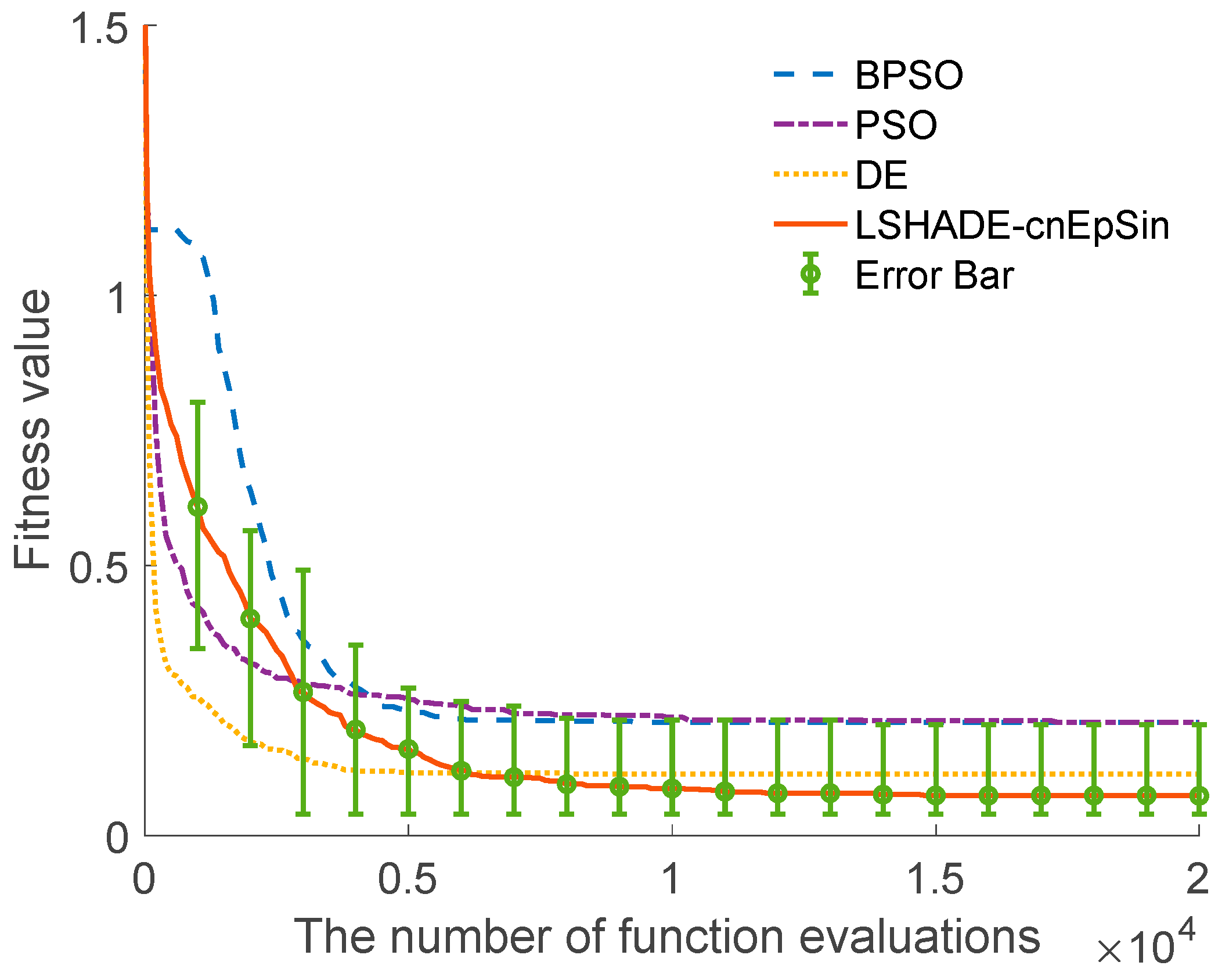
Figure 2 shows the convergence curves of the tested algorithms for the first learner with 200 materials in the database. Each curve is averaged on 30 independent runs. The error bars of LSHADE-
cnEpSin are also drawn every 1000 FEs.
The convergence curves show that BPSO and PSO have similar convergence precision, whereas PSO converges faster in the initial stage. DE has the fastest convergence and outperforms BPSO and PSO in the average quality of solutions. LSHADE-cnEpSin showed a moderate convergence behavior in the early stage, while it continuously improves the solution throughout the entire search history and obtains the best average performance.
Table 2 shows the success rate, averaged mean, average minimum, and standard deviation of 30 runs over 100 learners with 200 materials. The algorithm that found the best solution (with minimum cost function value) is counted as a success for each learner. If multiple algorithms obtain the best solution, they are all successful. The results show that LSHADE-
cnEpSin has the highest chance (80 times out of 100 learners) of finding the best solution for a random learner. The mean, minimum, and standard deviation of 30 runs are computed and averaged over 100 learners. The results show that LSHADE-
cnEpSin outperforms the other algorithms’ solution quality and search stability. Additionally, DE in continuous form outperforms the binary PSO as well.
Take the first learner as an example. With 200 materials, BPSO, DE, and LSHADE-
cnEpSin obtained the same best learning path, and the corresponding cost was 0.04. The details of the obtained learning path are shown in
Table 3. The leaner’s ability level is 0.4, and the three selected materials have difficulty levels of (0.6, 0.4, 0.4), which fit the learner’s ability level well. The learning objective consists of concepts No. 1, No. 5, No. 9, and No. 10, and the materials cover just enough concepts. The time required to complete the learning path is 5.34, which satisfies the learner’s expectation. The first material has no prerequisite, which is suitable for the beginning of the path. The second material requires concept No. 9 as the prerequisite, which is covered by the first material. The third material requires the first concept, which is covered by the second material. No prerequisite is violated. The learning style of the learner is rescaled to 15 levels. The learning style indicators (2, 0, −1, 5) mean that the learner is inclined to visual (with strength 2), is balanced in sensing/intuitive, sightly global (with strength 1), and more active (with strength 5). The selected materials do not seem to fit the learning style well. However, given the complex constraints of the learning objectives and the prerequisites, this path is the best we can find among the 200 materials in the database.
With the richness of the materials, the matching is expected to be better. The best learning path obtained by LSHADE-
cnEpSin when the number of materials reaches 5000 is shown in
Table 4. The cost for this path is 0.0228, which is 0.0172 smaller than the cost with 200 materials. The decrease in the cost has two reasons: (1) the difficulty levels are the same as the learner’s ability level, causing zero affinity function value; (2) The supported learning styles are closer to the learner’s, which reduces the related affinity function as well. The impact of the number of materials on the quality of constructed learning paths will be discussed next.
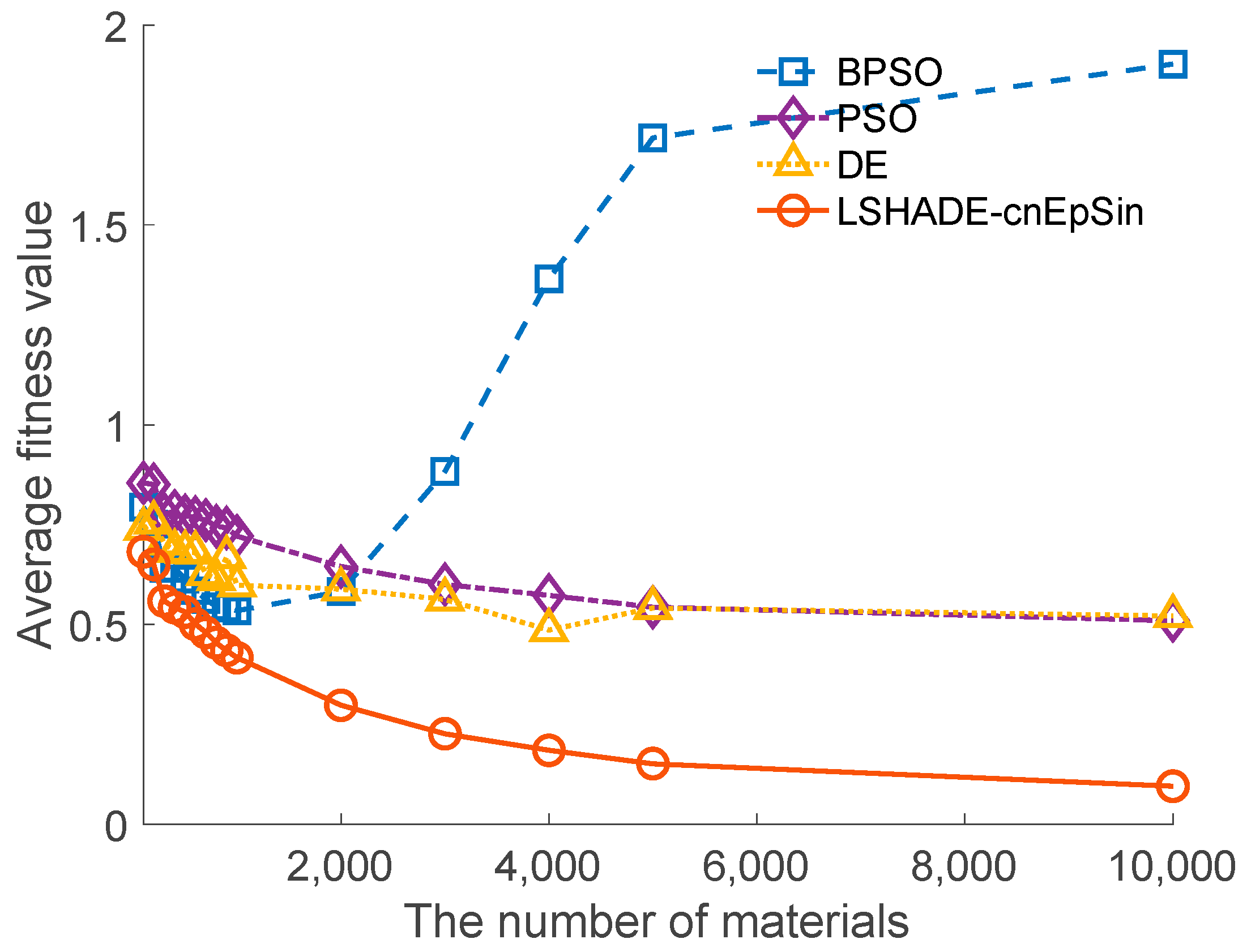
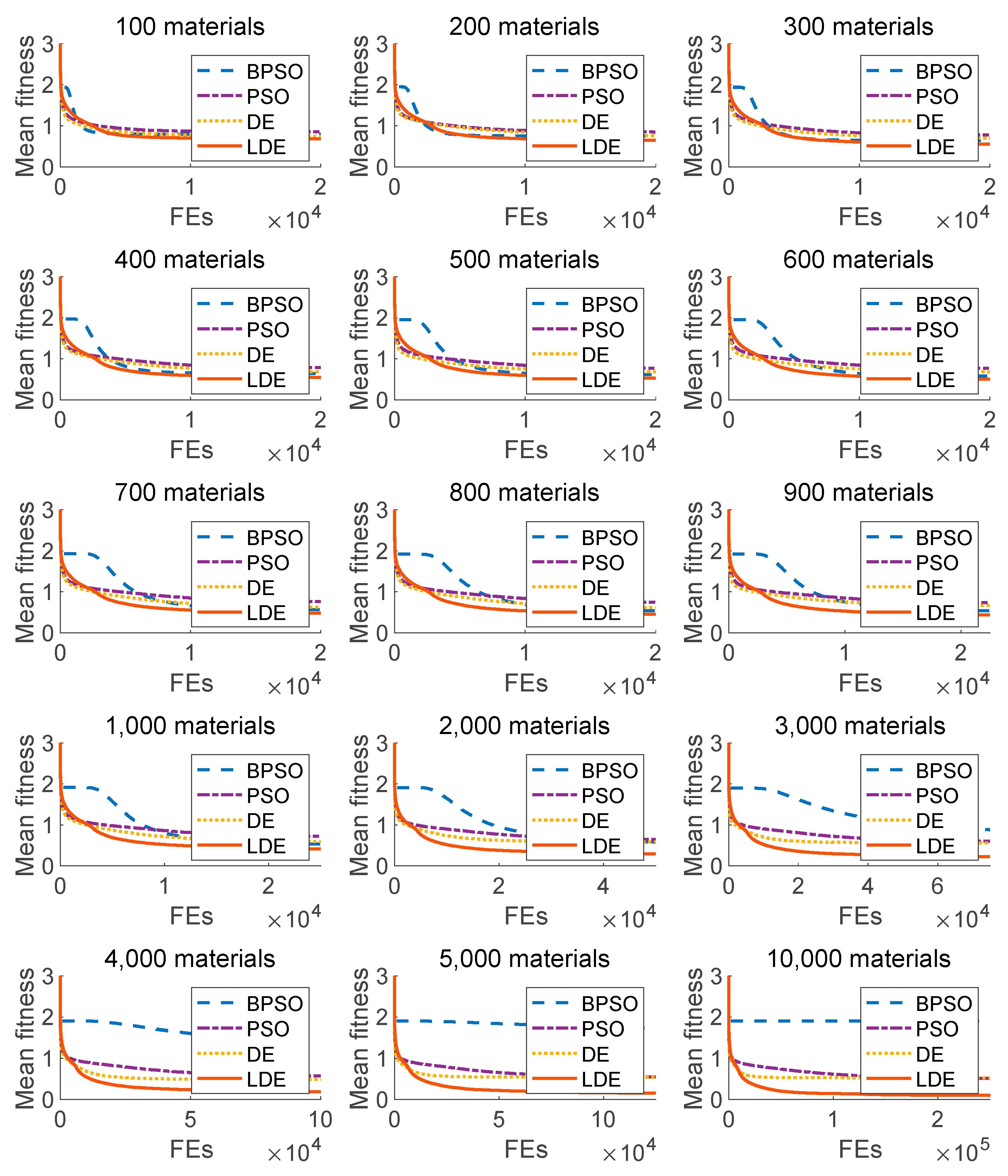
5.2. Influence of the Number of Materials
The number of materials may affect the performance of the binary algorithms since the search space grows with it. Whereas the increased richness of the materials may be beneficial for learning path planners as well. We tested the performance of BPSO, PSO, DE, and LSHADE-
cnEpSin with a different number of materials. The tested numbers of materials are 100, 200, …, 1000, 2000, …, 5000, and 10,000. For each number of materials, 30 runs are executed for each learner. The final cost function values are averaged on 30 runs and then on 100 learners. The results are shown in
Figure 3.
Figure 3 shows that with a limited number of materials (100 materials), all four algorithms obtain an average final fitness above 0.5. With such solution quality, one or more constraints may be violated. Especially for the learning style and material type, a mismatch is almost inevitable since the materials are not specifically designed for a single learner.
When the number of materials increases, all algorithms can improve their solutions. The turning point of the performance is 1000 materials. After this point, PSO and LSHADE-cnEpSin can improve the solutions further. The performance of DE seems less affected, whereas the performance of BPSO deteriorates with the number of materials.
The observation suggests that additional materials allow algorithms to explore more combinations of materials, hence increasing the possibility of producing better solutions for a learner. The search space does not increase with the number of materials for continuous algorithms with varying length representation. Therefore, an improvement in the solutions is expected. For binary representation, the search space increases exponentially with the number of materials. Thus, a performance bottleneck is observed when the problem scale reaches a certain point.
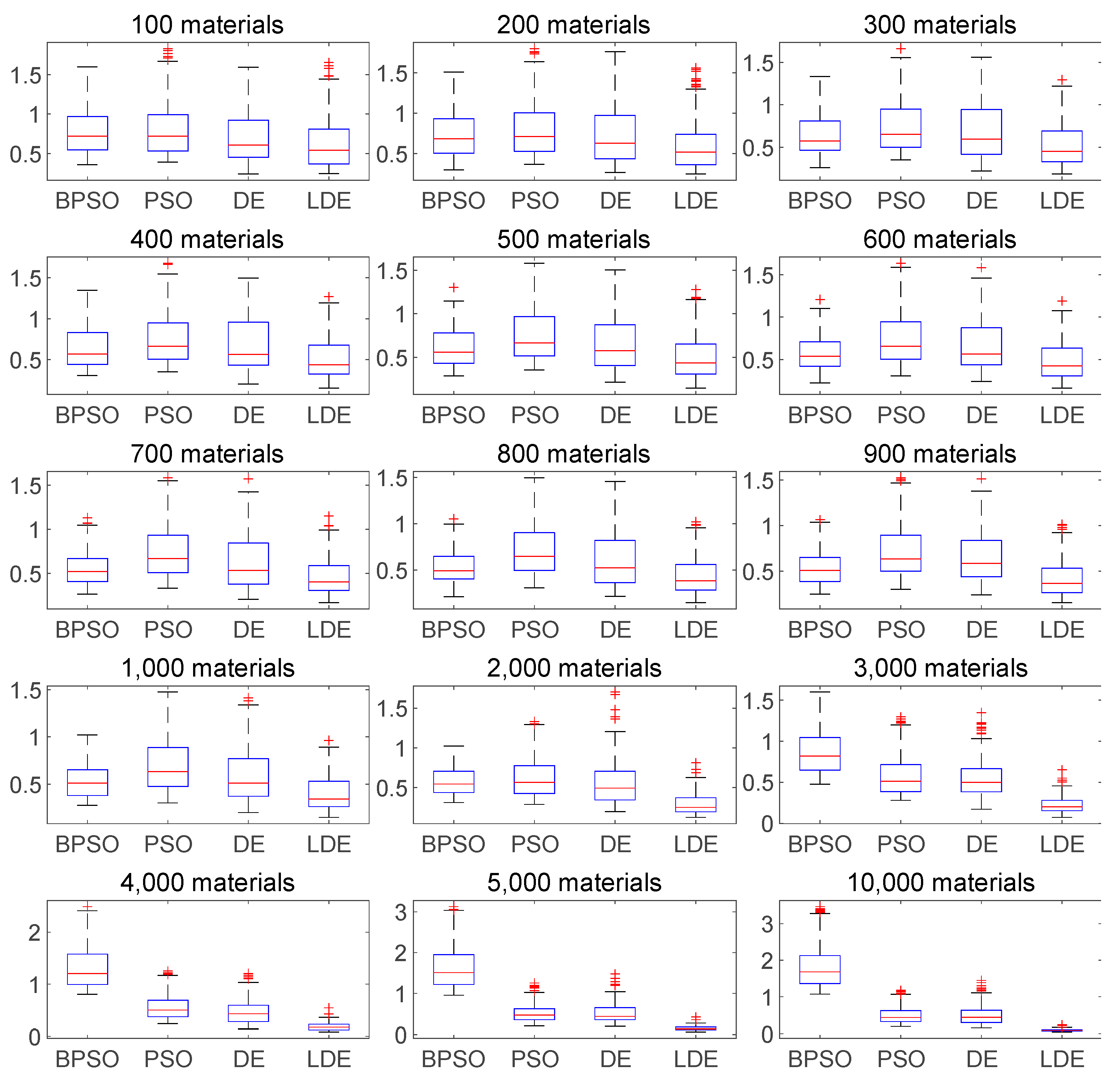
Figure 4 shows the boxplots of the final cost value of the tested algorithms (the LSHADE-
cnEpSin is labeled as ‘LDE’ for compactness). Each box shows the median (red line), percentiles, and outliers (red cross). The results show that LSHADE-
cnEpSin has better statistics for final solutions when the materials are rich.
Figure 5 shows the convergence curves of the four algorithms with a different number of materials. LSHADE-
cnEpSin (labeled as ‘LDE’ as well) shows an advantage when the number of materials exceeds 500, which becomes apparent when the materials exceed 1000.
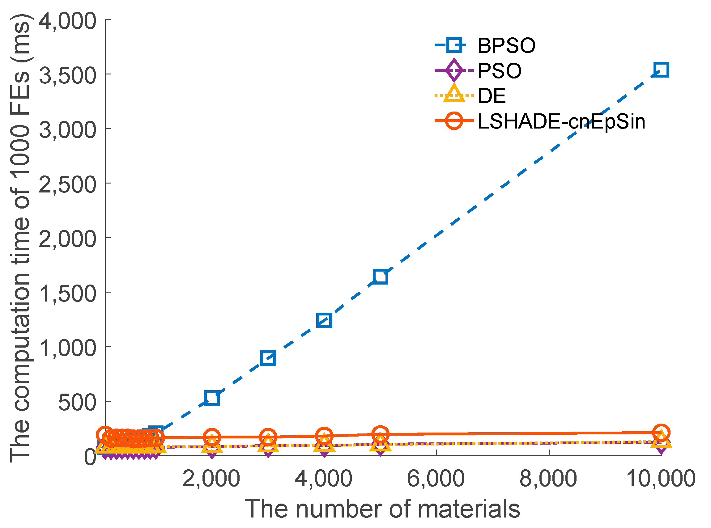
5.3. Scalability Analysis
The average computation time per 1000 function evaluations is in
Figure 6. The results show that the algorithms with varying length representation, i.e., PSO, DE, and LSHADE-
cnEpSin, require constant computation time for a different number of materials. Meanwhile, the algorithms with binary representation, i.e., BPSO, consumed computation time that increased linearly with the number of materials. LSHADE-
cnEpSin takes about 200 ms to complete 1000 function evaluations, almost twice the time compared to PSO and DE. The additional computation time of LSHADE-
cnEpSin is from the computation of Euclidean distance for each pair of individuals in a population and the subsequent coordinate transformation. Trading a constant extra computation time for improved performance seems a reasonable investment for the learning path problems.
6. Conclusions
This paper proposes a multi-attribute match (MAM) model for the learning path planning problem. The MAM model considers various aspects of both learners and learning materials. The attributes regarding a learner include the ability level, learning target, learning style, and expected learning time. The attributes regarding a learning material include difficulty level, covered concepts, supported learning style, required learning time, and prerequisite concepts. Five affinity functions are proposed to describe the relations between a learner and the learning path. The weighted sum of the affinity function is used as the cost function to be optimized by evolutionary algorithms.
A variable-length continuous representation (VLCR) of a learning path is proposed to utilize the powerful search ability of continuous evolution algorithms and reduce the search space. The numerical experiments show that the algorithms adopting the VLCR have comparable performance with the PSO adopting binary representation when the number of materials is smaller. When the number of materials is more than 1000, the performance of binary PSO starts to deteriorate. Eventually, BPSO fails to provide a valid solution if the number of materials exceeds 5000. In contrast, the number of materials has a limited influence on producing high-quality learning paths for the algorithms adopting the VLCR. The results show the high scalability of VLCR when combined with continuous evolutionary algorithms. Represented by the learning path planning problems, a series of practical problems with undetermined plan sizes, such as the location-allocation problem and the knapsack problem, may benefit from the flexibility of VLCR and the powerful search ability of continuous evolutionary algorithms.
Further, the constant computation time of VLCR shows the potential of dealing with large-scale learning path planning problems, which might be essential for a real-world learning management system that contains thousands of learning materials to generate a valid learning path before the learner loses patience. A practical application of the proposed model can be generating a learning path that contains materials from different courses. For a single course, the topic redundancy may be too low to replace any of the materials. Therefore, a learning path that covers all the concepts related to the course may contain all the materials, i.e., the length of the path is fixed. However, suppose there are many courses with similar topics to choose from. In that case, the topic redundancy becomes higher, and the search space becomes larger, for which a fixed-length solution representation that contains all the materials will be inefficient and VLCR will be suitable.
It is expected that MAM and VLCR will make an impact on real-world learning path planning problems. Learning is an interactive process between the learner and the materials. However, this research did not consider the time-varying attributes of learners, such as the acquired concepts or the learning performance throughout the learning process. Future work may include a dynamic learning path update using the interaction information of a learner, a collaborative filtering mechanism to improve the quality of the initial learning path, or a repetition mechanism of the materials that help the learner to memorize essential concepts.
Author Contributions
Conceptualization, Y.-W.Z.; methodology, Q.X.; software, Y.-W.Z.; validation, Y.-W.Z. and Y.-L.S.; formal analysis, Y.-W.Z.; investigation, M.-M.C.; resources, M.-M.C.; data curation, Y.-W.Z.; writing—original draft preparation, Y.-W.Z.; writing—review and editing, Q.X.; visualization, Y.-W.Z.; supervision, Y.-L.S.; project administration, M.-M.C.; funding acquisition, M.-M.C. All authors have read and agreed to the published version of the manuscript.
Funding
This research was funded by (1) Undergraduate Education and Teaching Reform Research Project of Jiangsu University of Science and Technology, 2021, Grant number: XJG2021015 (2) Postgraduate Instruction Cases Construction Project of Jiangsu University of Science and Technology “Optimal Control”, 2020, Grant number: YAL202003; (3) Construction Project of Postgraduate Online Courses of Jiangsu University of Science and Technology, 2020, Grant number: YKC202002; (4) Philosophy and Social Science Research Project for the Universities of Jiangsu Province “Research on the Personalized Design Strategy of Ubiquitous Learning Resources Based on the Learner Model”, 2019, Grant number: 2019SJA1912; (5) National Science Foundation of China, 2019, Grant number: 51875270. The APC was funded by Higher Education Project of Jiangsu University of Science and Technology “Research on Informatization Innovation Strategies Based on the Ecosystem of Adult Higher Education”, 2020, Grant number: GJKTYBJX202004.
Data Availability Statement
Conflicts of Interest
The authors declare no conflict of interest. The funders had no role in the design of the study; in the collection, analyses, or interpretation of data; in the writing of the manuscript; or in the decision to publish the results.
References
- Baidada, M.; Mansouri, K.; Poirier, F. Personalized E-Learning Recommender System to Adjust Learners’ Level. EdMedia+ Innovate Learning 2019, 1353–1357. [Google Scholar]
- Kausar, S.; Huahu, X.; Hussain, I.; Wenhao, Z.; Zahid, M. Integration of Data Mining Clustering Approach in the Personalized E-Learning System. IEEE Access 2018, 6, 72724–72734. [Google Scholar] [CrossRef]
- Vagale, V.; Niedrite, L.; Ignatjeva, S. Implementation of Personalized Adaptive E-Learning System. Balt. J. Mod. Comput. 2020, 8, 293–310. [Google Scholar] [CrossRef]
- Nabizadeh, A.H.; Leal, J.P.; Rafsanjani, H.N.; Shah, R.R. Learning Path Personalization and Recommendation Methods: A Survey of the State-of-the-Art. Expert. Syst. Appl. 2020, 159, 113596. [Google Scholar] [CrossRef]
- Nabizadeh, A.H.; Jorge, A.M.; Leal, J.P. RUTICO: Recommending Successful Learning Paths under Time Constraints. In Proceedings of the UMAP 2017—Adjunct Publication of the 25th Conference on User Modeling, Adaptation and Personalization, Bratislava, Slovakia, 9–12 July 2017; pp. 153–158. [Google Scholar] [CrossRef]
- Wu, M.Y.; Ke, C.K.; Lai, S.C. Optimizing the Routing of Urban Logistics by Context-Based Social Network and Multi-Criteria Decision Analysis. Symmetry 2022, 14, 1811. [Google Scholar] [CrossRef]
- Zhang, J.; Zhang, J.; Zhang, Q.; Wei, X. Obstacle Avoidance Path Planning of Space Robot Based on Improved Particle Swarm Optimization. Symmetry 2022, 14, 938. [Google Scholar] [CrossRef]
- Yao, J.; Li, X.; Zhang, Y.; Ji, J.; Wang, Y.; Liu, Y. Path Planning of Unmanned Helicopter in Complex Dynamic Environment Based on State-Coded Deep Q-Network. Symmetry 2022, 14, 856. [Google Scholar] [CrossRef]
- Chu, C.P.; Chang, Y.C.; Tsai, C.C. PC2PSO: Personalized e-Course Composition Based on Particle Swarm Optimization. Appl. Intell. 2011, 34, 141–154. [Google Scholar] [CrossRef]
- Christudas, B.C.L.; Kirubakaran, E.; Thangaiah, P.R.J. An Evolutionary Approach for Personalization of Content Delivery in E-Learning Systems Based on Learner Behavior Forcing Compatibility of Learning Materials. Telemat. Inform. 2018, 35, 520–533. [Google Scholar] [CrossRef]
- Hssina, B.; Erritali, M. A Personalized Pedagogical Objectives Based on a Genetic Algorithm in an Adaptive Learning System. Procedia Comput. Sci. 2019, 151, 1152–1157. [Google Scholar] [CrossRef]
- Dwivedi, P.; Kant, V.; Bharadwaj, K.K. Learning Path Recommendation Based on Modified Variable Length Genetic Algorithm. Educ. Inf. Technol. 2018, 23, 819–836. [Google Scholar] [CrossRef]
- Elshani, L.; Nuçi, K.P. Constructing a Personalized Learning Path Using Genetic Algorithms Approach. arXiv 2021, arXiv:2104.11276. [Google Scholar]
- Awad, N.H.; Ali, M.Z.; Suganthan, P.N. Ensemble Sinusoidal Differential Covariance Matrix Adaptation with Euclidean Neighborhood for Solving CEC2017 Benchmark Problems. In Proceedings of the 2017 IEEE Congress on Evolutionary Computation (CEC), Donostia, Spain, 5–8 June 2017; pp. 372–379. [Google Scholar]
- Peng, H.; Ma, S.; Spector, J.M. Personalized Adaptive Learning: An Emerging Pedagogical Approach Enabled by a Smart Learning Environment. Lect. Notes Educ. Technol. 2019, 171–176. [Google Scholar] [CrossRef]
- Zhang, Y. Intelligent Recommendation Model of Contemporary Pop Music Based on Knowledge Map. Comput. Intell. Neurosci. 2022, 2022, 1756585. [Google Scholar] [CrossRef] [PubMed]
- Zhong, D.; Fan, J.; Yang, G.; Tian, B.; Zhang, Y. Knowledge Management of Product Design: A Requirements-Oriented Knowledge Management Framework Based on Kansei Engineering and Knowledge Map. Adv. Eng. Inform. 2022, 52, 101541. [Google Scholar] [CrossRef]
- Chen, X.; Jia, S.; Xiang, Y. A Review: Knowledge Reasoning over Knowledge Graph. Expert Syst Appl 2020, 141, 112948. [Google Scholar] [CrossRef]
- Zhou, J.; Jiang, G.; Du, W.; Han, C. Profiling Temporal Learning Interests with Time-Aware Transformers and Knowledge Graph for Online Course Recommendation. Electron. Commer. Res. 2022, 1–21. [Google Scholar] [CrossRef]
- Diao, X.; Zeng, Q.; Li, L.; Duan, H.; Zhao, H.; Song, Z. Personalized Learning Path Recommendation Based on Weak Concept Mining. Mob. Inf. Syst. 2022, 2022, 2944268. [Google Scholar] [CrossRef]
- Pinandito, A.; Prasetya, D.D.; Hayashi, Y.; Hirashima, T. Design and Development of Semi-Automatic Concept Map Authoring Support Tool. Res. Pract. Technol. Enhanc. Learn. 2021, 16, 1–19. [Google Scholar] [CrossRef]
- Gao, P.; Li, J.; Liu, S. An Introduction to Key Technology in Artificial Intelligence and Big Data Driven E-Learning and e-Education. Mob. Netw. Appl. 2021, 26, 2123–2126. [Google Scholar] [CrossRef]
- Sarkar, S.; Huber, M. Personalized Learning Path Generation in E-Learning Systems Using Reinforcement Learning and Generative Adversarial Networks. In Proceedings of the 2021 IEEE International Conference on Systems, Man, and Cybernetics (SMC), Melbourne, Australia, 17–20 October 2021; pp. 92–99. [Google Scholar] [CrossRef]
- Benmesbah, O.; Lamia, M.; Hafidi, M. An Enhanced Genetic Algorithm for Solving Learning Path Adaptation Problem. Educ. Inf. Technol. 2021, 26, 5237–5268. [Google Scholar] [CrossRef]
- Son, N.T.; Jaafar, J.; Aziz, I.A.; Anh, B.N. Meta-Heuristic Algorithms for Learning Path Recommender at MOOC. IEEE Access 2021, 9, 59093–59107. [Google Scholar] [CrossRef]
- Shi, D.; Wang, T.; Xing, H.; Xu, H. A Learning Path Recommendation Model Based on a Multidimensional Knowledge Graph Framework for E-Learning. Knowl. Based Syst. 2020, 195, 105618. [Google Scholar] [CrossRef]
- Lin, C.F.; Yeh, Y.C.; Hung, Y.H.; Chang, R.I. Data Mining for Providing a Personalized Learning Path in Creativity: An Application of Decision Trees. Comput. Educ. 2013, 68, 199–210. [Google Scholar] [CrossRef]
- Jugo, I.; Kovačić, B.; Slavuj, V. Using Data Mining for Learning Path Recommendation and Visualization in an Intelligent Tutoring System. In Proceedings of the 2014 37th International Convention on Information and Communication Technology, Electronics and Microelectronics (MIPRO), Opatija, Croatia, 26–30 May 2014; pp. 924–928. [Google Scholar] [CrossRef]
- Vanitha, V.; Krishnan, P.; Elakkiya, R. Collaborative Optimization Algorithm for Learning Path Construction in E-Learning. Comput. Electr. Eng. 2019, 77, 325–338. [Google Scholar] [CrossRef]
- Al-Muhaideb, S.; Menai, M.E.B. Evolutionary Computation Approaches to the Curriculum Sequencing Problem. Nat. Comput. 2011, 10, 891–920. [Google Scholar] [CrossRef]
- Storn, R.; Price, K. Differential Evolution—A Simple and Efficient Heuristic for Global Optimization over Continuous Spaces. J. Glob. Optim. 1997, 11, 341–359. [Google Scholar] [CrossRef]
- Wang, F.; Zhang, L.; Chen, X.; Wang, Z.; Xu, X. A Personalized Self-Learning System Based on Knowledge Graph and Differential Evolution Algorithm. Concurr. Comput. 2022, 34, e6190. [Google Scholar] [CrossRef]
- Chen, C.A.; Chiang, T.C. Adaptive Differential Evolution: A Visual Comparison. In Proceedings of the 2015 IEEE Congress on Evolutionary Computation (CEC), Sendai, Japan, 25–28 May 2015; pp. 401–408. [Google Scholar] [CrossRef]
- Li, Y.; Wang, H.; Wang, N.; Zhang, T. Optimal Scheduling in Cloud Healthcare System Using Q-Learning Algorithm. Complex Intell. Syst. 2022, 8, 4603–4618. [Google Scholar] [CrossRef]
- Wang, H.; Yan, Q.; Wang, J. Blockchain-Secured Multi-Factory Production with Collaborative Maintenance Using Q Learning-Based Optimisation Approach. Int. J. Prod. Res. 2021. [Google Scholar] [CrossRef]
- Yan, Q.; Wang, H. Double-Layer Q-Learning-Based Joint Decision-Making of Dual Resource-Constrained Aircraft Assembly Scheduling and Flexible Preventive Maintenance. In IEEE Transactions on Aerospace and Electronic Systems; IEEE: New York, NY, USA, 2022; pp. 1–18. [Google Scholar] [CrossRef]
- Huynh, T.N.; Do, D.T.T.; Lee, J. Q-Learning-Based Parameter Control in Differential Evolution for Structural Optimization. Appl. Soft Comput. 2021, 107, 107464. [Google Scholar] [CrossRef]
- Zhang, J.; Sanderson, A.C. JADE: Self-Adaptive Differential Evolution with Fast and Reliable Convergence Performance. In Proceedings of the 2007 IEEE Congress on Evolutionary Computation (CEC), Singapore, 25–28 September 2007; pp. 2251–2258. [Google Scholar] [CrossRef]
- Tanabe, R.; Fukunaga, A. Success-History Based Parameter Adaptation for Differential Evolution. In Proceedings of the 2013 IEEE Congress on Evolutionary Computation (CEC), Cancun, Mexico, 20–23 June 2013; pp. 71–78. [Google Scholar] [CrossRef]
- Tanabe, R.; Fukunaga, A.S. Improving the Search Performance of SHADE Using Linear Population Size Reduction. In Proceedings of the 2014 IEEE Congress on Evolutionary Computation (CEC), Beijing, China, 6–11 July 2014; pp. 1658–1665. [Google Scholar] [CrossRef]
- Awad, N.H.; Ali, M.Z.; Suganthan, P.N.; Reynolds, R.G. An Ensemble Sinusoidal Parameter Adaptation Incorporated with L-SHADE for Solving CEC2014 Benchmark Problems. In Proceedings of the IEEE Congress on Evolutionary Computation (CEC), Vancouver, BC, Canada, 24–29 July 2016; pp. 2958–2965. [Google Scholar]
- Zhang, Y.W.; Xiao, Q.; Sun, X.Y.; Qi, L. Comparative Study of Swarm-Based Algorithms for Location-Allocation Optimization of Express Depots. Discrete Dyn. Nat. Soc. 2022, 2022, 3635073. [Google Scholar] [CrossRef]
- Felder, R.M.; Silverman, L.K. Learning and Teaching Styles In Engineering Education. Eng. Educ. 1988, 78, 674–681. [Google Scholar]
- Zhang, J.; Sanderson, A.C. JADE: Adaptive Differential Evolution with Optional External Archive. IEEE Trans. Evol. Comput. 2009, 13, 945–958. [Google Scholar] [CrossRef]
- Wang, Y.; Li, H.X.; Huang, T.; Li, L. Differential Evolution Based on Covariance Matrix Learning and Bimodal Distribution Parameter Setting. Appl. Soft Comput. J. 2014, 18, 232–247. [Google Scholar] [CrossRef]
- Punjabi, M.; Prajapati, G.L. Enhancing Performance of Lazy Learner by Means of Binary Particle Swarm Optimization. In Proceedings of the 2021 IEEE International Conference on Technology, Research, and Innovation for Betterment of Society (TRIBES), Raipur, India, 17–19 December 2021. [Google Scholar] [CrossRef]
- Shi, Y.; Eberhart, R. A Modified Particle Swarm Optimizer. In Proceedings of the IEEE International Conference on Evolutionary Computation (CEC), Anchorage, AK, USA, 4–9 May 1998; pp. 69–73. [Google Scholar]
- Li, P.; Yang, J. PSO Algorithm-Based Design of Intelligent Education Personalization System. Comput. Intell. Neurosci. 2022, 2022, 9617048. [Google Scholar] [CrossRef]
| Publisher’s Note: MDPI stays neutral with regard to jurisdictional claims in published maps and institutional affiliations. |
© 2022 by the authors. Licensee MDPI, Basel, Switzerland. This article is an open access article distributed under the terms and conditions of the Creative Commons Attribution (CC BY) license (https://creativecommons.org/licenses/by/4.0/).


