A Hierarchy of Interactions between Pathogenic Virus and Vertebrate Host

Abstract

This review is of basic models of the interactions between a pathogenic virus and vertebrate animal host. The interactions at the population level are described by a predatory-prey model, a common approach in the ecological sciences, and depend on births and deaths within each population. This ecological perspective is complemented by models at the genetical level, which includes the dynamics of gene frequencies and the mechanisms of evolution. These perspectives are symmetrical in their relatedness and reflect the idealized forms of processes in natural systems. In the latter sections, the general use of deep learning methods is discussed within the above context, and proposed for effective modeling of the response of a pathogenic virus in a pathogen–host system, which can lead to predictions about mutation and recombination in the virus population.

1. Introduction

The sections that follow employ basic models of ecology and evolution to illustrate interactions between a pathogenic virus and a vertebrate animal host. It is not a systematic review of the literature, but instead a focused review of virus–host dynamics by use of a basic population model of predator-prey mechanics and their dynamics at the genetical level. To complement this traditional thinking on population biology, there are sections on the plausibility of a machine learning method for modeling the genetic changes that lead to new viral variants.

2. Population-Based Approach to the Virus–Host Interaction

There are varieties of viruses that depend on the cells of a vertebrate host. These virus types may be classified according to their genetic material, such as whether their genetic package is composed of the nucleic acid DNA or RNA. These types may be further subdivided by molecular structure, including their strandedness and mechanism of replication. These forms of viruses are also associated with a genomic size and rate of replication error [1]. The evolution of these viral forms is constrained by the above, along with other biological factors, such as the physical constraint of genomic packaging inside a protein capsid shell [2]. Where the packaging is highly constrained, then evolution will tend to favor genes that overlap with one another along the genome, so that any given genomic region may code for multiple gene products [3].

However, the deeper evolutionary relationships among these viral types are not easily discerned since there is not a canonical and conserved set of genes for simple classification, and even within a single viral subtype, the relationships among the subtype populations are often obscured by high rates of evolution at the genetic level. Therefore, it is not applicable to apply the same assumptions for constructing a virus phylogeny as in constructing the phylogenetic relationships of animals where the populations are potentially distinct with clear patterns of divergence [4].

A virus type and its physical characteristics impact its population dynamics and evolution [5]. In the case of a viral pathogen, the interactions with a host are a major cause of its population level responses and the evolution of its genes [5,6,7,8]. This perspective is at the population level, in contrast to that of molecular pathways, such as viral replication and the corresponding responses in the host immune system. The advantage of a population level perspective is the availability of mathematical rigor in modeling a population as a set of discrete particles, accompanied by recovery of its behavior in an ecological context, including spatial and temporal dimensions. This can lead to robust predictions about the population responses, as opposed to a subjective assessment based on few or a larger number of biased observations.

The above approaches of ecology and evolution provide insight and intuition into population responses, a robust perspective that is juxtaposed to extrapolation of cellular level processes for describing population level phenomena. Instead, the probabilism of population based thinking is essential for testing hypotheses. The alternative is to rely on determinism and weak assumptions about population responses, such as the influence of sampling effects that occur in the genetics of populations. An example of a sampling effect is where a population with few individuals is less resistant to extinction than one with a larger population size.

3. Model of Virus–Host Interactions at the Population Level

3.1. Description of the Model

It is favorable to first employ simple models for testing scientific hypotheses, and consequently avoiding too many unknown factors. One relatively simple model of ecology is illustrated in the Lotka–Volterra model of predator-prey interactions [9,10,11,12,13]. This model also is applicable to an interaction between parasite and its host, given they have responses that are consistent with the definition of a predator and prey. There are two equations in the model [14], one for the numerical response of the predator (P) and the other for that of the prey (H):

dH/dt = rH − pHP

(1)

dP/dt = a(pHP) − dP

(2)

In the above equations, the values of dH/dt and dP/dt represent the rate of prey and predator population growth, respectively. An exponential model of population growth, where there is an acceleration in the number of individuals added to a single population, instead of a two population model, is represented by the equation dN/dt = rN. In the case of the prey population of the predator-prey model, the parameter N is replaced by H, so the equivalent equation that excludes prey deaths, but includes births, is dH/dt = rH.

Equation (1) shows this exponential function for prey birth rate, rH. However, the Lotka–Volterra model also requires a set of parameters to estimate the death rate. In the case of the prey population, the death rate is represented by pHP, where HP corresponds to the rate of interactions between the predator and prey, and an opportunity for the predator to consume the prey. An additional parameter, p, represents the probability that this interaction actually leads to consumption of the prey by the predator, therefore, the prey death rate is shown as pHP.

The birth rate of the predator population is solely dependent on consumption of the prey, so the prey death rate (pHP) is then used for estimating the predator birth rate, but with an additional parameter, a, for representing the proportion of prey material that is available for offspring predator production, while the remaining matter and energy is used elsewhere, such as in non-digestible biological material, or for fueling the metabolism in adult predators. Therefore, a(pHP), the product of prey consumed by predator, and the proportion available toward offspring production, represents the value of the actual birth rate for predators. The death of predators is not dependent on the predator-prey interactions, so this rate is estimated by a prior, dP, where P is the predator predator population size and d is the estimate of their death rate.

In the case of a parasite-host interaction, as in a virus–host interaction, the Lotka–Volterra model is applicable where a set of assumptions hold true. One assumption is the presence of two populations in the system, one whose role is the predator and the other the prey. In the virus–host interaction, the pathogenic virus is the predator and the prey is the host, where this special case restricts the host to members of the clade of vertebrate animals. However, the host must be susceptible to infection by the virus to participate in the system. Each viral infection is further assumed to be a binary value, either a full infection or not infected.

The birth rate in the prey population, which corresponds to the host, is rH and shows an exponential rate of growth in the susceptible host population. An assumption here is that host immunity is decaying at a rate of r. In this case, the decay in host immunity has two major causes, one is the decrease in the effectiveness of the host immune system against the pathogenic virus, while the second is evolution of the virus for its achieving resistance to host immunity.

The prey growth equation includes a parameter for deaths in addition to births, as described above. The death rate is specified by pHP. The product HP corresponds to the interactions between a virus-susceptible host (H) and a virus (P). The other parameter is p, which represents the probability of a viral infection in the host, and removal of the host from the population as defined by virus-susceptible members. This may be caused by factors other than death of the host, such as recovery from infection, including an immune response to viral infection.

Likewise, the virus has a rate of births in the model. It is a(pHP), representing successful infections in the host population (pHP), along with a parameter a, which represents the conversion of the infection to production of new viral pathogens. However, an assumption is that the progeny are capable at infecting the host population. Lastly, there is a death rate for the virus population, dP, where d is the estimated death rate and P is the virus population size. The death rate also includes individuals that can no longer infect a host since members are defined by this attribute (infection susceptibility). Another assumption of the model is a viral subpopulation in any host is considered as a single particle, or individual. The viral infection is not modeled as a population process once it enters a host. This can be considered a separate process from infection, at least for a design of a simple model for insight into population biology.

Where the model’s predictions do not correspond to observation in natural populations, then other hypotheses may be generated to explain the phenomena. The model also has fewer assumptions as opposed to complex models that are expected to have many assumptions about the populations and the natural environment. Another benefit of the Lotka–Volterra model is the theory can substitute for lack of robust data otherwise not available in natural populations.

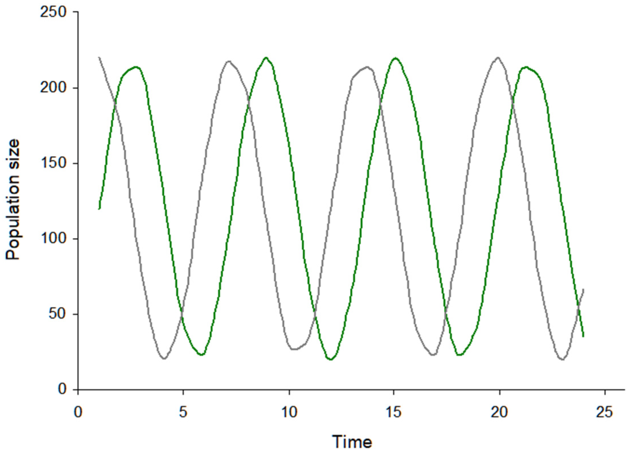
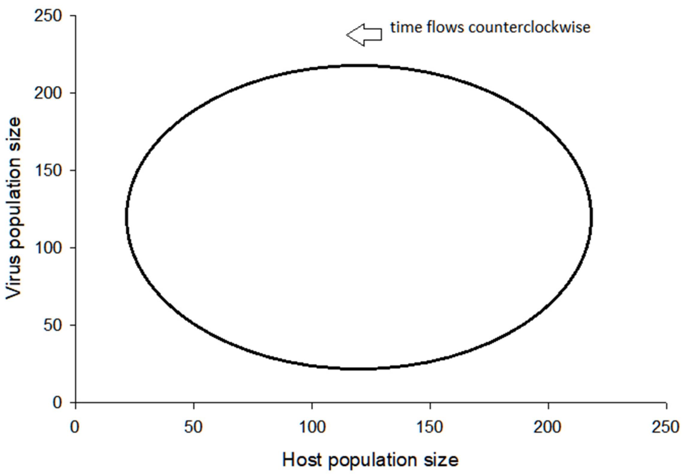
3.2. Visualization of the Virus–Host Model

Figure 1 is a sinusoidal plot of the predator-prey population dynamic, where the pathogenic virus and vertebrate host populations are fluctuating in size over time. The rates of these changes are described by the Lotka–Volterra equations. These population fluctuations are mathematically described, and are a consequence of population interaction between virus and host. The system is further confined as isolated to external factors, such as a second interacting host population in the system.

A central characteristic in Figure 1 is the time lag in the population response, and that the population dynamics are not synchronized with time. Where the time delay is smaller, these population oscillations are dampened. Likewise, with a larger time delay, the oscillations become larger.

Figure 2 is a plot of the population dynamics of predator and prey. Instead of displaying the populations as separate plots, as in the Figure 1, both populations are shown together in this case. The plot shows a population cycling and the long-term stability in the system. If the cycle increases in size, then the chance increases that a population may crash. If this occurs, then the system collapses and no further changes can occur in either of the populations.

Instability in the predator-prey system occur by a variety of natural processes. In the case of a virus–host interaction, instability can be caused by a lack of response by evolutionary change in the pathogenic virus population, given that the vertebrate host is responding by acquiring immunity to resist the virus. This occurrence would lead to a lack of susceptible hosts (Figure 3). A different scenario is where the virus is evolving, but the vertebrate host is not adapting by acquiring immunity to the virus, and, therefore, the host population is more likely to collapse (Figure 3). In a case that is intermediate between these two scenarios, where the virus is evolving and the host is acquiring immunity, then the system may persist over time, along with the expected population oscillations.

The range of possible population responses vary. In the case of a stable system with a low rate of genetic change in the virus population, and given the susceptible host population is infrequently infected, or slowly acquiring immunity, then the population oscillations will increase in size. For the common Influenza viruses, these population dynamics coincide with the seasonal changes, and, therefore, the population responses typically occur over a span of weeks or longer.

The above model shows that a virus population size can reach zero, for the case where a population crashes or is otherwise no longer participating in the system, such as where the vertebrate host population acquires immunity. However, this model also has an assumption of spatial homogeneity in the distribution of its population (Figure 4A).

If instead the host population is heterogeneous in its spatial distribution, then it is expected that these populations have greater resistance to collapse (Figure 4B) [15]. However, this model is not applicable where there is more than one host in the system. If the virus predates on other vertebrate animal hosts, particularly if the species are taxonomically distant, then the virus is expected to maintain its population over a longer time period since the populations are spatially heterogeneous [15]. Likewise, an assumption of spatial homogeneity corresponds to a fairly uniform distance between individuals, but a heterogeneous pattern has a broader distribution where the expected distance is potentially greater among individuals, so, in the case of a prey population, there is a greater opportunity for hiding from predators (Figure 5). This effectively deters destabilization in this two population system.

Lastly, the heterogeneity in population distribution can also occur along the temporal dimension. If the host population has individuals that are moving over time across their geographical location, then this effect is expected to lead to clustering of individuals, and potentially decrease the probability of interaction between the predator and prey.

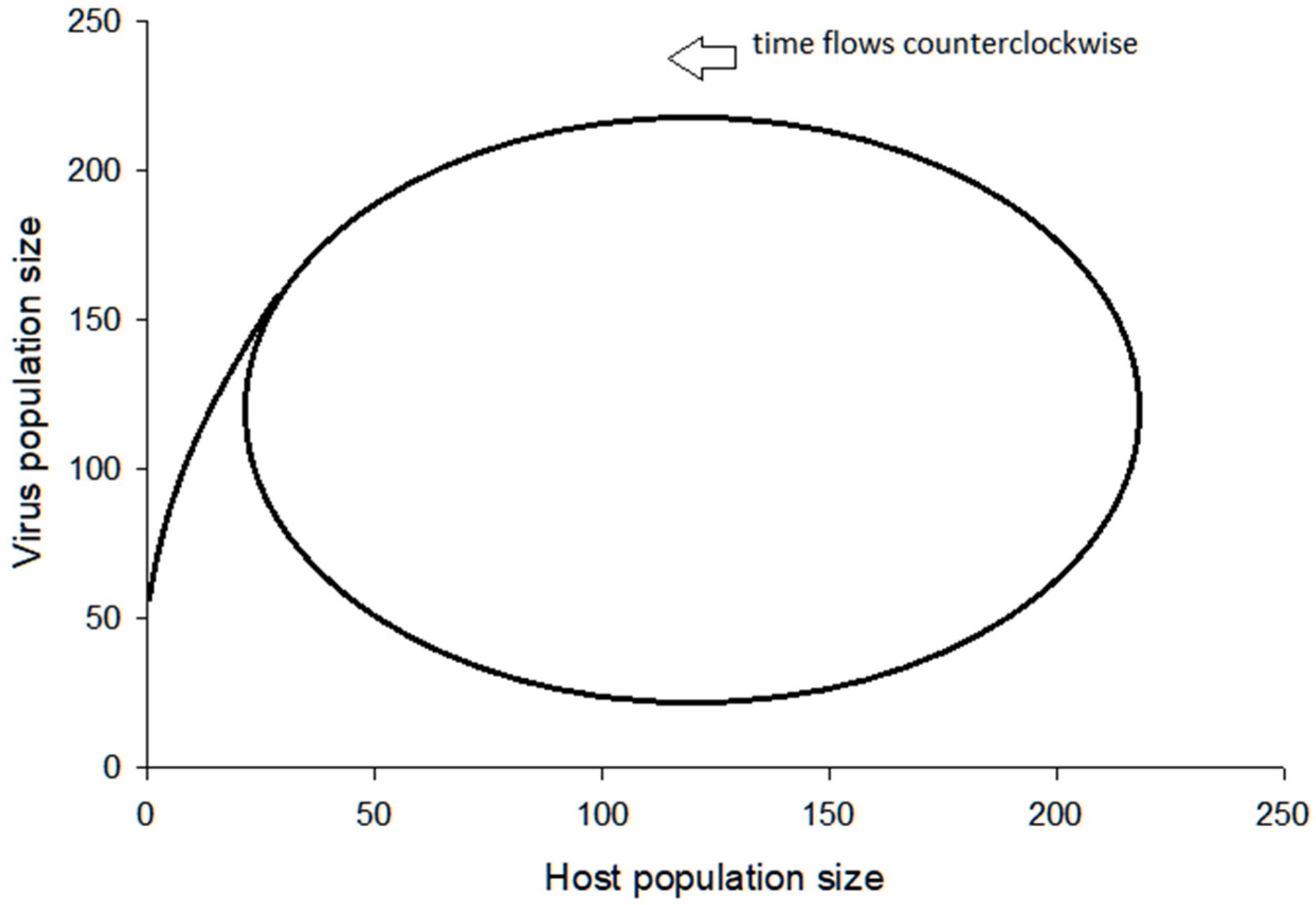
3.3. Further Comments on Virus–Host System Instability

The above section introduces causes of instability in the virus–host population system. These causes include factors related to the evolution of new viral genotypes and the population distributions. Both of these phenomena are a result of evolutionary and ecological effects. However, these two kinds of effects are intertwined in population systems [6,7]. For instance, with a change in the natural environment, such as a change in the climatic conditions, then there exists an ecological factor that influences the virus–host system, and the factor may interact with the population responses by the virus and host. This is an additional layer of complexity for modeling the system, but is relevant for anticipating the virus–host dynamics that occur in Nature. Otherwise, oversimplication in the design of a model may lead to false expectations, particularly where the model is not robust to the missing parameters.

This is particularly relevant where associating population dynamics at the genetic level with the observed phenotypic traits. The dynamics involve factors associated with both ecology and evolution. An example of evolutionary factors is expectations on mutation and recombination rates in the populations, while ecological factors may include population distribution and interactions with the natural environment [6,7].

These systems are, at their essence, a contest of response times. Given the constraints in a virus–host system, then a delay in one of the population responses may lead to collapse of the system. If the delay is exceedingly long in comparison to the average response, then it is expected that the system will collapse. Persistence and stability of the system is increased where particular constraints are removed in the virus–host model, such as the inclusion of another host that is susceptible to the virus. Another form of escape is for the virus to more rapidly explore the space of adaptive changes and overcome any population response by the host. This may involve the mechanism of genetic recombination which complements the role of mutation in the evolutionary (and ecological) contest where the host is also responding by generation of immunity by a somatic form of recombination.

4. Model of Virus–Host Interactions at the Genetic Level

In a conventional predatory-prey interaction, the predator population responds by an increase in offspring production where the rate of growth is increasing in the prey population. Likewise, the pathogenic virus population is expected to respond by a positive growth rate with an increase in the number of susceptible vertebrate hosts. The growth in number of susceptible hosts occurs by many causes. The causes include an inadequate immune response and decay of immunity from prior virus infection.

At the mechanistic level, the vertebrate host responds by immunity at the somatic level. This response is largely based on creating a diverse number of protein receptors on dedicated immune cells. These cellular specific receptors are diverse in their protein structure as a result of mutational and recombinational processes along segments of genes in the genome of the somatic cell. However, in the case of the virus, it is expected to respond at an evolutionary level, otherwise this predator-prey system would tend toward instability, and collapse, since the availability of hosts is expected to decrease as they acquire immunity or the infection leads to host extinction. Another scenario is that the host survives with some loss of immunity and the unchanged virus type subsequently reinfects the host. This event is highly unlikely since the virus is undergoing evolution, such as by mutation, a process that is inescapable for any genetic molecule subjected to the physical processes occurring across the Earth’s biosphere.

Another factor affecting virus population response is genetic heterogeneity (Figure 6) [6,7]. If the virus population has high genetic heterogeneity (Figure 6B), then the virus is expected to have a higher chance of infecting a virus-susceptible host population. Vertebrate host populations in Nature are genetically heterogeneous, particularly in molecules that interact with pathogenic peptides, therefore, this heterogeneity is probably a necessary component as a defense against intracellular pathogens [6]. Likewise, a pathogenic virus population with higher genetic variation is expected to grant Nature a greater opportunity to select for variants with higher fitness.

Emergence of a new viral genotype that rises relatively rapidly in the population is an example of the natural selection process of evolution. Although small populations may have a non-beneficial viral variant rise in frequency by chance, this process is expected to occur over a much longer time period (slow evolutionary rate). In the case where the natural selection process occurs repeatedly [16], then a large number of new or rare mutations are expected to become common in the population (high evolutionary rate).

Since the evolutionary process in small populations is not dominated by natural selection, the dynamics of gene frequencies will tend to produce non-beneficial or harmful effects in protein encoded genes (Figure 7A); the accumulation of these particular mutations will tend to lower the overall fitness of members of the population [17]. Recombination is an evolutionary process to escape from this dilemma and compensate for the accumulation of deleterious mutations, and, therefore, new genotypes are more easily formed with higher fitness (Figure 7B). These are probabilistic processes dependent on sampling effects in the population.

The shape and function of a protein is dependent on its underlying sequence of amino acids. The biological set of amino acids cluster by their chemical properties, therefore, some amino acid changes have less impact on the protein than others. In addition, for a nucleic acid sequence that codes for a protein, some of the nucleic acid changes do not result in an amino acid change (Figure 8), so it can be stated that the coding of amino acids by nucleic acids is buffered against the effects of mutation [18]. This is a piece of evidence for the high likelihood for the harmful effects of mutation, particularly in mutation that affects the protein sequence. Other evidence includes observation in the rates of evolution, where populations strongly disfavor amino acid change as compared to nucleic acid change that does not change the protein sequence [17].

5. Models for Generation of Protein Sequences

5.1. Overview of Deep Learning Methods

The deep learning methods of computer science, based on a complex form of an artificial neural network, are capable of modeling nonlinear dynamical systems, including the case with a very large number of parameters as observed in many natural systems. These methods deploy a neural network as a program for modeling the transformation of a sequence of input data to that of a known output sequence. The model is trained during a training step, typically by an implementation of backpropagation and gradient descent. After the program is trained, then it can generate an expected output sequence given the prior input of sequence data. This program may be further described as a model that can make predictions about complex natural systems, however, the robustness of the model is frequently dependent on very large collections of data and an appropriate deep learning architecture. Furthermore, the architecture and hyperparameters of a deep learning system are tunable components that are pivotal in developing a robust model. The tuning of a deep learning architecture is typically handled as a series of experiments since there is not a sufficient theoretical framework to serve as a substitute.

As a program, the artificial neural network expects to receive and output data as a binary encoded sequence, such as illustrated by the example value 01100011. However, a data set of interest is not often in a binary number format, so the non-binary data requires conversion to binary data. In the case of a protein sequence, each amino acid may be first converted to the common one letter format; for example, MGGATIY. Each letter or letters are equivalent to potential tokens that altogether form a sequence for input to an artificial neural network (Figure 9) [19,20,21]. In addition, attributes of each amino acid may be appended as tokens to each of the tokens based on the amino acids along the sequence. Ofer and others ([20] p. 1753) review the utility of these methods for tokenization of protein sequence data, and for the attributes of amino acids, such as their participation in two dimensional protein structure.

Deepmind’s AlphaFold [21,22] applies this kind of tokenization method and a deep learning architecture for rendering predictions of three dimensional protein structure. Its training step includes prior input data in the form of amino acid sequences of proteins, sets of priors in the form of three dimensional protein structures, and the biochemical and geometrical features, including the spatial orientation of each amino acid and values for the rotatable bonds (Supplementary Materials of [21], p. 8).

5.2. Deep Learning Models of Protein Structure

The concept that structure and function are entangled together is a common observation in natural science, including in the anatomical features of organisms and at the level of biological molecules [23]. In the case of proteins, their three dimensional structure is expected to mirror biological function. The capability of modeling this three dimensional structure of a sequence is crucial for making predictions on processes, such as in the pathways of vertebrate immunity.

In particular, the adaptive immune response in vertebrate animals is dependent on detection of a pathogenic organism, including the disease-causing viruses. The detection and learning processes occur at the molecular level, including pathways for splicing proteins originating from self and those of foreign sources. Recognition of foreign peptides is dependent on a polymorphic receptor at the surface of a specialized type of immune cell and the display of the peptide by a different cell surface receptor (Figure 10) [24,25,26,27]. The proximate cause of recognition of pathogens is the display of the three dimensional structure of the cell surface receptor as bound together with the pathogenic protein subsequence [24], where the binding results from a pocket in the receptor along with forces of weak molecular interactions between the molecules [28]. Predictions on these molecular processes allow for predictions on the outcomes as influenced by adaptive immunity; and, therefore, this is a powerful insight into virus–host interactions.

Many of the salient and discrete pathways of adaptive immunity are modeled at some level of certainty [29,30]. However, models such as Deepmind’s AlphaFold are limited in their predictions of protein structure where there is a complicating factor in modeling the higher-order intermolecular interactions. The major conceptual problems to solve include robust prediction of the cellular receptor protein structure while bound with a foreign peptide, the binding affinity of a peptide to a given cellular receptor, and which peptides are generated by the formal cell-based splicing process.

Deep reinforcement learning is one approach for evaluating virus evolution as a response to the effects of a vertebrate host and its adaptive immune system. This kind of methodology represents a Markov decision process, in a general sense, and is a trial and error process for achieving the highest measurable reward among trials [31,32]. These trials may include the set of possible viral protein sequences as defined by evolution, including those caused by mutation and genetic recombination, and where each of the sequences is evaluated against the pathways of host immunity. Specifically, these sequences serve as the reinforcement learning agent, where each agent explores the environment consisting of the challenges by the host’s adaptive immune system. Each round of exploration results in a reward value measuring the degree of immune evasion by a virus. Reinforcement learning could lead to a neural network that is trained to model protein sequence evolution of the virus, and its interaction with the pathway of interest in the vertebrate host immune system.

In general, the deep learning approaches are refined by experimentation, so they depend on trial and error in finding an ideal architecture and for achieving a plausible level of biological realism. Deep reinforcement learning offers a single framework for modeling virus evolution and ecology, but it is also valid for investigating the steps of the pathways of the vertebrate host immune system. The deep learning models for predicting three dimensional protein structure are particularly applicable for understanding virus evolution in evading host cell detection at the molecular level, so this is probably a better approach to understanding the system than by collecting vast amounts of data necessary to generate viral variants from prior knowledge of viral genomes and their effects on vertebrate immunity. This latter effort is fraught with unknowns, such as the capability in broad sampling across all host species, along with the relevant metrics to measure the immune response in the hosts. However, the following section describes a deep learning architecture for validation of the broad sampling problem.

6. A Deep Learning Model for Generating Protein Sequences

6.1. GPT-2 as a Model for Sequence Generation

GPT-2 is a deep learning architecture to generate text from a corpus, a prior collection of text documents [33]. This architecture is implemented on a few major components, the deep learning component, the data component, and the computer hardware. GPT-2 relies on a deep learning framework based on the formal transformer architecture, an algorithm that is optimal for hardware acceleration and in creating statistical associations among non-local portions of a sequence. In particular, the ProtGPT2 model [34] extends GPT-2 for generation of protein sequences.

ProtGPT2 relies on the GPT-2 architecture, specifically GPT-2-XL, for deep learning, and the UniRef50 protein sequence collection for the data component [33,35]. The hardware requirements for training the model are steep. They reportedly used 128 specialized processors (GPUs) for completing model training over the span of several days. However, the requirements would be much higher if the prior data was based on UniProt’s UniRef100 sequence collection since UniRef50 defines and excludes redundant sequences based on relaxed criteria of sequence similarity [35]. In general, the UniRef data sets are optimized for searches of sequence similarity, and, as a result, offer increased interpretability for the results of a search [35]. However, by design, UniRef50 does not have broad coverage of virus sequence data. In the case of DeepMind’s AlphaFold, the source of protein sequences is similarly based on the UniProt data, specifically UniRef90 [21].

GPT-2 is currently a favored deep learning system for generation of text, particularly because it has the necessary decoder component of the transformer architecture [36], and has modifications for language modeling, such as masked self-attention [33]. It has another advantage, its transformer architecture is accessible by a software library released by Huggingface, and includes a programming interface (API) with the Python language, and open source license for use of their code [37]. One method to test this API is by use of the Google Colab service [38] which has a web-based interface to remote computer hardware, including the use of hardware accelerators (GPUs) for training large models. However, ProtGPT2 is dependent on GPT-2-XL, a version of GPT-2 with over a billion parameters [34]. This larger model may exceed the memory limit of the Colab service, whereas a few hundred million parameter model is less likely to exceed this limit. There are also other remote services at Google, and those offered by other companies, for purchasing blocks of time for access to servers and GPUs. Purchasing remote access in blocks of time is a cost efficient method to train deep learning models.

6.2. Large Data Collections for Training Deep Learning Models

Large collections of protein sequences, including those of viruses, are available at internet sites, such as the NCBI RefSeq collection [39]. This collection is web browseable at ftp.ncbi.nlm.nih.gov/genomes/refseq (accessed on 5 September 2022). In its subdirectories, the Fasta formatted sequence data are associated with text based descriptions across files in Genbank Protein Format. These files are often split into many compressed files, so it is typically necessary to uncompress the files before concatenating them so as to create a single data file for use as input. The data may have a lot of redundant sequences, a potential problem addressed by UniProt’s UniRef databases. A preprocessing step should include identification of redundant sequences for potential deletion.

The predictive power of deep learning models is dependent on the prior data, in this case the protein sequences. It is important to consider including a broad sample of protein sequences to potentially capture the types of amino acid modifications that are common in a protein. This refers to those modifications that result from point mutation. It will also be useful to sample depthwise for sequences related to the desired prediction. These practices are expected to contribute to power to predict the expected occurrence of amino acids along the sequence. In other words, it is not only the amount of data, but also the quality. This is a theme that also resonates in modeling of natural language.

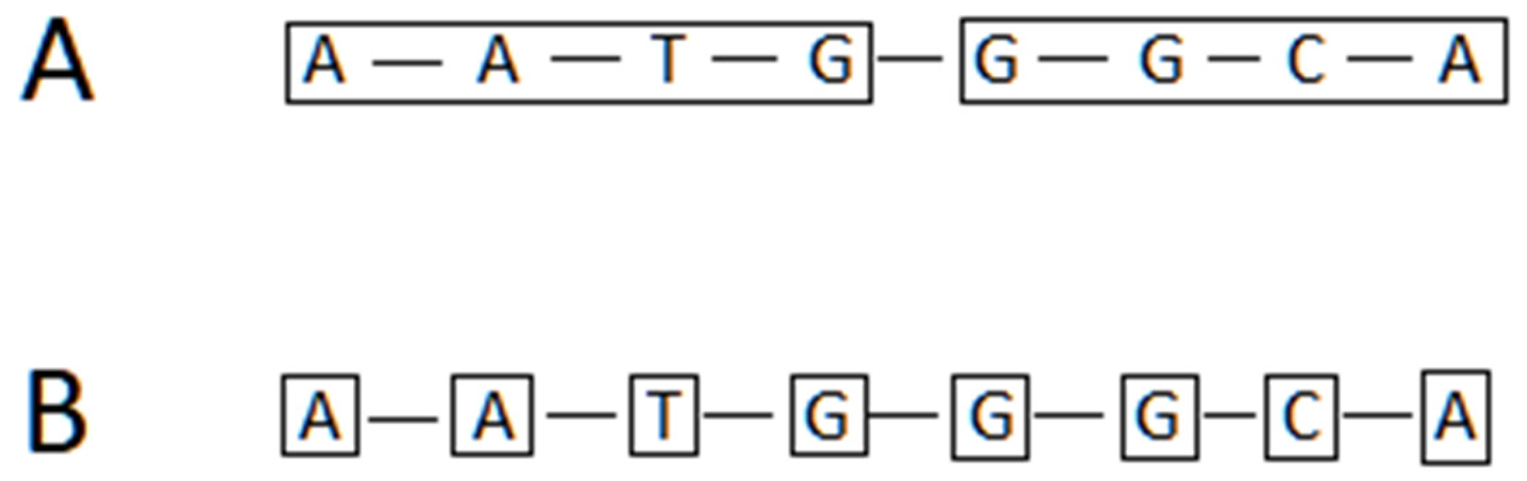
6.3. Approaches for Tokenization of Protein Sequence Data

The generation of protein sequences by deep learning, at least that based solely on prior sequence data, is sensitive to the input data and the vocabulary of tokens. The input data has to be validated against its representation of its taxa and their genes. For example, if a gene of interest codes for a keratin protein in a mouse, but the database has sparse representation of the keratin gene family in mammals, then the tokens and trained model will not have a robust ability to generate a diverse and robust set of keratin protein sequences. A related problem is whether the prior sequence data captures protein evolution at the amino acid level. This requires a lot of data for capturing a general model of protein evolution. The language models, such as GPT-2, capture a large base of potential words in sentences by creating a vocabulary on the order of tens of thousands. However, the amino acids in protein sequences can form many more “words” than a common written language. If the tokens do not provide a sufficient sample for the model to generate sequence data, then the model will produce poor results.

In the case of AlphaFold’s model of three dimensional protein structure, there are many input features, including tokenization of the properties of the amino acids. One of the properties is aatype, an “one-hot representation of the input amino acid sequence” (Supplementary Materials of [21], p. 8). However, in the case of ProtGPT’s generative model, the use of tokens typically represent several amino acids (Figure 9). This procedure does not constrain its ability in generating a diverse set of protein sequences since the goal is to create a diversity of proteins as constrained by the prior vocabulary. In the case of fine-scale prediction of sequence data, it may be a better practice to assign tokens to single amino acids by training the tokenizer to a vocabulary where each token is assigned to a single amino acid. This is good practice where the goal is sequence prediction that reflects the protein evolution, particularly for point mutation and its fixation in the population. In addition, with a very large and diverse data set, and a many-layered transformer, the model is expected to capture the higher level interactions in a protein sequence, such as the spatial interactions between non-adjacent amino acids.

For the tokenization step, The Huggingface API includes a function for training a byte-pair encoding tokenizer on data [37]. The code for the tokenizer has a parameter for vocabulary size, which influences model training and the model’s parameter size.

6.4. A Procedure for Generating Protein Sequences

The deep learning architecture is a neural network of nodes, where each connection between nodes has an assigned weight. During a training step that includes both input and output values, the neural network and its weight values are trained to computationally transform the input values to their expected output values. This trained neural network is then used as a model to make predictions, given the applicability of the hypothesized model and a set of prior input values. At a mechanistic level, this is an abstract computational process based on binary numbers. However, from a higher level perspective, it is perceptually a powerful tool for constructing novel images, paragraphs of text, and spatial structure of proteins. In the case of of protein sequence generation, the procedure includes the procedural steps of tokenization of the data, training of the model, and prediction of tokens by first prompting with prior text input.

Tokenization is a transformation of any data source to a token format. For protein sequences, each of the sequences may be defined as a single unit of interest, similar to language modeling where the unit is a word or a sentence [34,40]. To achieve this aim, a method is to flank each of the sequences with a token for the beginning-of-sequence and end-of-sequence. For GPT-2, these two tokens appear as <|endoftext|> [37]. Likewise, each sequence is recoded to a sequence of tokens. This is also a transformational process in conversion of non-binary data to a form of input as expected by an artificial neural network.

The assignment of tokens is an algorithm. GPT-2, and likewise ProtGPT2, use byte pair encoding (BPE) that is available in the Huggingface library [37]. BPE compresses the sequence data by a lossless algorithm to a sequence of bytes [41]. The ideal result of the tokenization step is to identify the most commonly used word roots while dividing the rarer words into subwords [34,41]. In the case of protein sequence data, the data are divided into subsequences, a kind of subword of amino acids. Many of these subsequences are a common occurrence in the data, while the BPE algorithm may also identify the rarer subsequences in the data set. In the case of ProtGPT2, BPE was employed on a smaller dataset from the Swiss-Prot database, and resulted in the assignment of over 50,000 tokens, where an average token is a subsequence of four amino acids, representable by a numerical value.

The above method considers each protein sequence as a single unit. As an alternative method of tokenization, each amino acid can be considered as a single unit, as in the case for a word in a sentence in a language model. To test this method, the data would be formatted so that each amino acid is followed by a space character, and the prediction step would also use this format for its input.

In GPT-2, the model training step relies on the tokens created above for assignment to a dataset of interest. The model is then trained on the tokenized data. The model used for this case is GPT2LMHeadModel [37]. The subsequent step of protein sequence generation is dependent on this trained model. The model is expected to be sensitive to data sampling and parameter specification, so a robust model depends on repeated modification and testing of the procedure.

Input of any sequence, such as a subsequence beginning with a start codon, will lead to a generation of tokens in a sequence, a process dependent on an algorithm that searches for generating the most probable token. This occurs sequentially along the sequence during the prediction step. These generated tokens faithfully correspond to the underlying protein sequence data, so the tokens are interconvertible with the protein sequence. I uploaded example code at GitHub for testing, modifying, and implementing the above steps [42].

7. Discussion

The above sections discuss simple and general models of virus evolution. First, the predator-prey model, as applied to the special case of a pathogen–host interaction, a mathematical model of population dynamics. Second, evolutionary models are discussed for a foundation on how a virus evolves in a virus–host system. These models are specific to interactions between a pathogenic virus and its vertebrate host; although there is related literature on generalized models of antagonistic coevolution in populations, including for populations without an adaptive immune system [6,7]. In the remaining sections, deep learning is a topic as a predictive model of virus evolution. These methods are based on assumptions about sampling of data and parameterization, as expected in any formal model. Altogether, the above different approaches in population biology are symmetrical in that they are related to one another, and in combination lead to insight on natural populations.

The deep learning architectures are capable of modeling complex natural systems where trained on very large data sets [43,44,45]. In the case of viruses, if there is a vast and diverse data set of sequences that correspond to the viral peptides, along with knowledge of their interactions with the molecules of vertebrate host immunity, then it is possible for deep learning to capture and model the high dimensional features of proteins, such as properties of their three dimensional structure. This approach is related and symmetrical with that used in language models created by deep learning.

Even though it is simple to measure a distance between two related protein sequences, the distance between proteins at the three dimensional level is a higher order of complexity. However, there is a symmetry between these measurements since the structure of proteins is dependent on its primary sequence. For a virus to evade the adaptive immune system in the host, it would rely on evolution to find mutants that alter the shape of the original protein or proteins. The dynamics of protein shape and conformation is a key process in predicting the success of a virus population in evading a host immune system.

Immune cell surveillance of viral peptides, in the case of vertebrate animals, is dependent on a complex model since these cellular receptors are diverse, undergo a selection process in the host, and act in a combinatorial fashion for detection of foreign peptides. There is also an expectation that this detection process is probabilistic and the strength of detection is finely graded by dependence on multiple factors, including in the participation by multiple receptor types, and the strength of each detection event at the molecular level. A deterministic perspective may lead to the naive notion that adaptive immunity functions as a simple set of switches, but instead the probabilistic aspects of adaptive immunity lead to a variable response built upon molecular level interactions.

The above examples show the symmetry among the various spatial scales of a protein, including its higher order structure. The relevant functions of the host immune system are dependent on protein structure, just as protein function in other biological processes emerge from the associated structure of the protein. This relationship leads to a reflection on the importance of modeling three dimensional structure from the protein sequence, and extending these models for prediction of the structure while they are interacting with other molecules.

Even though past deep learning approaches have often depended on priors related to protein structure data, it may also be of interest in modeling protein structure as a bottom-up process that starts with the physical forces at the atomic level. This is a potential method where the protein structure data is not fully capturing the representations that correspond to structure at the atomic level. Clearly, the number of parameters to capture this model is unknown, it may be that the number is very large, therefore, it is of interest to validate the robustness of any model. This suggestion is for work beyond models of relatively basic protein structure, and to extend models to the higher order molecular interactions, as is relevant to the population-level contest in a virus–host system.

References

1. Campillo-Balderas, J.A.; Lazcano, A.; Becerra, A. Viral genome size distribution does not correlate with the antiquity of the host lineages. Front. Ecol. Evol. 2015, 3, 143. [Google Scholar] [CrossRef] [Green Version]
2. Sun, S.; Rao, V.B.; Rossmann, M.G. Genome packaging in viruses. Curr. Opin. Struct. Biol. 2010, 20, 114–120. [Google Scholar] [CrossRef] [Green Version]
3. Chirico, N.; Vianelli, A.; Belshaw, R. Why genes overlap in viruses. Proc. R. Soc. B Biol. Sci. 2010, 277, 3809–3817. [Google Scholar] [CrossRef] [Green Version]
4. Nasir, A.; Romero-Severson, E.; Claverie, J.M. Investigating the Concept and Origin of Viruses. Trends Microbiol. 2020, 28, 959–967. [Google Scholar] [CrossRef]
5. Obermeyer, F.; Jankowiak, M.; Barkas, N.; Schaffner, S.F.; Pyle, J.D.; Yurkovetskiy, L.; Bosso, M.; Park, D.J.; Babadi, M.; MacInnis, B.L.; et al. Analysis of 6.4 million SARS-CoV-2 genomes identifies mutations associated with fitness. Science 2021, 376, 1327–1332. [Google Scholar] [CrossRef]
6. Hamilton, W.D.; Axelrod, R.; Tanese, R. Sexual reproduction as an adaptation to resist parasites (A Review). Proc. Natl. Acad. Sci. USA 1990, 87, 3566–3573. [Google Scholar] [CrossRef] [Green Version]
7. Agrawal, A.; Lively, C.M. Infection genetics: Gene-for-gene versus matching-alleles models and all points in between. Evol. Ecol. Res. 2002, 4, 91–107. [Google Scholar]
8. Anderson, R.M.; May, R.M. Coevolution of hosts and parasites. Parasitology 1982, 85, 411–426. [Google Scholar] [CrossRef]
9. Lotka, A.J. Analytical note on certain rhythmic relations in organic systems. Proc. Natl. Acad. Sci. USA 1920, 6, 410–415. [Google Scholar] [CrossRef] [Green Version]
10. Lotka, A.J. Contribution to the mathematical theory of capture: I. Conditions for capture. Proc. Natl. Acad. Sci. USA 1932, 18, 172–178. [Google Scholar] [CrossRef] [Green Version]
11. Volterra, V. Fluctuations in the abundance of a species considered mathematically. Nature 1926, 118, 558–560. [Google Scholar] [CrossRef]
12. Volterra, V. Variazioni e fluttuazioni del numero d’individui in specie animali conviventi. Mem. Della R. Accad. Naz. Dei Lincei 1926, 2, 31–113. [Google Scholar]
13. Kingsland, S.; Alfred, J. Lotka and the origins of theoretical population ecology. Proc. Natl. Acad. Sci. USA 2015, 112, 9493–9495. [Google Scholar] [CrossRef] [PubMed] [Green Version]
14. Anisiu, M.C. Lotka, Volterra and their model. Didact. Math. 2014, 32, 9–17. [Google Scholar]
15. Huffaker, C. Experimental studies on predation: Dispersion factors and predator-prey oscillations. Hilgardia 1958, 27, 343–383. [Google Scholar] [CrossRef] [Green Version]
16. Simonsen, K.L.; Churchill, G.A.; Aquadro, C.F. Properties of statistical tests of neutrality for DNA polymorphism data. Genetics 1995, 141, 413–429. [Google Scholar] [CrossRef]
17. Kimura, M. The Neutral Theory of Molecular Evolution. Sci. Am. 1979, 241, 98–129. [Google Scholar] [CrossRef]
18. Freeland, S.J.; Hurst, L.D. The Genetic Code Is One in a Million. J. Mol. Evol. 1998, 47, 238–248. [Google Scholar] [CrossRef]
19. Hie, B.; Zhong, E.D.; Berger, B.; Bryson, B. Learning the language of viral evolution and escape. Science 2021, 371, 284–288. [Google Scholar] [CrossRef]
20. Ofer, D.; Brandes, N.; Linial, M. The language of proteins: NLP, machine learning & protein sequences. Comput. Struct. Biotechnol. J. 2021, 19, 1750–1758. [Google Scholar]
21. Jumper, J.; Evans, R.; Pritzel, A.; Green, T.; Figurnov, M.; Ronneberger, O.; Tunyasuvunakool, K.; Bates, K.; Žídek, A.; Potapenko, A.; et al. Highly accurate protein structure prediction with AlphaFold. Nature 2021, 596, 583–589. [Google Scholar] [CrossRef] [PubMed]
22. Marcu, S.-B.; Tabirca, S.; Tangney, M. An Overview of Alphafold’s Breakthrough. Front. Artif. Intell. 2022, 5, 875587. [Google Scholar] [CrossRef] [PubMed]
23. Wainwright, S.A. Form and Function in Organisms. Am. Zool. 1988, 28, 671–680. [Google Scholar] [CrossRef] [Green Version]
24. Klein, J.; Figueroa, F. Evolution of the major histocompatibility complex. Crit. Rev. Immunol. 1986, 6, 295–386. [Google Scholar] [CrossRef]
25. Davis, M.M.; Bjorkman, P.J. T-cell antigen receptor genes and T-cell recognition. Nature 1988, 334, 395–402. [Google Scholar] [CrossRef]
26. Germain, R.N. MHC-dependent antigen processing and peptide presentation: Providing ligands for T lymphocyte activation. Cell 1994, 76, 287–299. [Google Scholar] [CrossRef]
27. Friedman, R. A Perspective on Information Optimality in a Neural Circuit and Other Biological Systems. Signals 2022, 3, 410–427. [Google Scholar] [CrossRef]
28. Garstka, M.A.; Fish, A.; Celie, P.H.; Joosten, R.P.; Janssen, G.M.; Berlin, I.; Hoppes, R.; Stadnik, M.; Janssen, L.; Ovaa, H.; et al. The first step of peptide selection in antigen presentation by MHC class I molecules. Proc. Natl. Acad. Sci. USA 2015, 112, 1505–1510. [Google Scholar] [CrossRef] [Green Version]
29. O’Donnell, T.J.; Rubinsteyn, A.; Laserson, U. MHCflurry 2.0: Improved Pan-Allele Prediction of MHC Class I-Presented Peptides by Incorporating Antigen Processing. Cell Syst. 2020, 11, 42–48. [Google Scholar] [CrossRef]
30. Montemurro, A.; Schuster, V.; Povlsen, H.R.; Bentzen, A.K.; Jurtz, V.; Chronister, W.D.; Crinklaw, A.; Hadrup, S.R.; Winther, O.; Peters, B.; et al. NetTCR-2.0 enables accurate prediction of TCR-peptide binding by using paired TCR and sequence data. Commun. Biol. 2021, 4, 1060. [Google Scholar] [CrossRef]
31. Beattie, C.; Koppe, T.; Duenez-Guzman, E.A.; Leibo, J.Z. DeepMind Lab2D. arXiv 2020, arXiv:2011.07027. [Google Scholar]
32. Silver, D.; Singh, S.; Precup, D.; Sutton, R.S. Reward is enough. Artif. Intell. 2021, 299, 103535. [Google Scholar] [CrossRef]
33. Radford, A.; Wu, J.; Child, R.; Luan, D.; Amodei, D.; Sutskever, I. Language Models are Unsupervised Multitask Learners. Available online: openai.com/blog/better-language-models;github.com/openai/gpt-2 (accessed on 5 September 2022).
34. Ferruz, N.; Schmidt, S.; Hocker, B. ProtGPT2 is a deep unsupervised language model for protein design. Nat. Commun. 2022, 13, 4348. [Google Scholar] [CrossRef]
35. Suzek, B.E.; Huang, H.; McGarvey, P.; Mazumder, R.; Wu, C.H. UniRef: Comprehensive and non-redundant UniProt reference clusters. Bioinformatics 2007, 23, 1282–1288. [Google Scholar] [CrossRef] [PubMed] [Green Version]
36. Vaswani, A.; Shazeer, N.; Parmar, N.; Uszkoreit, J.; Jones, L.; Gomez, A.N.; Kaiser, Ł.; Polosukhin, I. Attention Is All You Need. In Proceedings of the 31st Conference on Neural Information Processing System, Long Beach, CA, USA, 4–9 December 2017; pp. 5998–6008. [Google Scholar]
37. Wolf, T.; Debut, L.; Sanh, V.; Chaumond, J.; Delangue, C.; Moi, A.; Cistac, P.; Rault, T.; Louf, R.; Funtowicz, M.; et al. Transformers: State-of-the-Art Natural Language Processing. In Proceedings of the 2020 Conference on Empirical Methods in Natural Language Processing: System Demonstrations, Online, 16–20 November 2020; pp. 38–45. [Google Scholar]
38. Bisong, E. Google Colaboratory. In Building Machine Learning and Deep Learning Models on Google Cloud Platform; Apress: Berkeley, CA, USA, 2019. [Google Scholar]
39. O’Leary, N.A.; Wright, M.W.; Brister, J.R.; Ciufo, S.; Haddad, D.; McVeigh, R.; Rajput, B.; Robbertse, B.; Smith-White, B.; Ako-Adjei, D.; et al. Reference sequence (RefSeq) database at NCBI: Current status, taxonomic expansion, and functional annotation. Nucleic Acids Res. 2016, 44, D733–D745. [Google Scholar] [CrossRef]
40. Bai, H.; Shi, P.; Lin, J.; Tan, L.; Xiong, K.; Gao, W.; Liu, J.; Li, M. Semantics of the Unwritten: The Effect of End of Paragraph and Sequence Tokens on Text Generation with GPT2. arXiv 2020, arXiv:2004.02251. [Google Scholar]
41. Gage, P. New Algorithm for Data Compression. C Users J. 1994, 12, 23–38. [Google Scholar]
42. Generative Model for Protein Sequences. Available online: github.com/bob-friedman/protein-sequence-generation (accessed on 4 September 2022).
43. Madani, A.; McCann, B.; Naik, N.; Keskar, N.S.; Anand, N.; Eguchi, R.R.; Huang, P.-S.; Socher, R. ProGen: Language Modeling for Protein Generation. arXiv 2020, arXiv:2004.03497. [Google Scholar]
44. Wu, K.; Yost, K.E.; Daniel, B.; Belk, J.A.; Xia, Y.; Egawa, T.; Satpathy, A.; Chang, H.Y.; Zou, J. TCR-BERT: Learning the grammar of T-cell receptors for flexible antigen-xbinding analyses. bioRxiv 2021. [Google Scholar] [CrossRef]
45. Park, M.; Seo, S.W.; Park, E.; Kim, J. EpiBERTope: A sequence-based pre-trained BERT model improves linear and structural epitope prediction by learning long-distance protein interactions effectively. bioRxiv 2022. [Google Scholar] [CrossRef]
Figure 1. Plot of population dynamics in the two population system with a pathogenic virus and a vertebrate animal host. The green color line corresponds to the pathogenic virus population, while the grey color corresponds to the vertebrate host. The population dynamics originate from the Lotka–Volterra model. For example, with an increase in virus population size, the susceptible host population undergoes a decrease in size. Furthermore, the oscillations are asynchronous, reflective of the lag in time for each of the populations to respond to the other.
Symmetry 14 02274 g001
Figure 2. Cycling of pathogenic virus and vertebrate animal host populations. This result is determined by the Lotka–Volterra model of a predator-prey interaction, and the cycle persists indefinitely, given the assumptions of the model are not violated.
Symmetry 14 02274 g002
Figure 3. Cycling in the the sizes of two populations, including the pathogenic virus and vertebrate animal host. The cycle does not persist indefinitely in this example, but instead the cycle collapses, and the host population size reaches zero. Without any susceptible hosts to infect, then the virus population will consequently collapse.
Symmetry 14 02274 g003
Figure 4. (A). An abstract view of a population with individuals that are uniformly distributed. This illustrates an example of spatial homogeneity in a population. (B). The individuals of a population are not uniformly distributed. This is an example of spatial heterogeneity.
Symmetry 14 02274 g004
Figure 5. The plot represents a virus–host interaction, and shows that as the vertebrate host population increases in spatial or temporal heterogeneity, then the average chance of the virus–host interaction decreases. Likewise, as the heterogenity decreases, and, therefore, the host population becomes more homogeneous, then the average chance of a virus–host interaction increases. This effect illustrates the concept of predator avoidance by prey hiding from detection.
Symmetry 14 02274 g005
Figure 6. (A). The circle represents a population, and the grey color boxes are the individuals with the same genotype. (B). In this case, the genotypes vary among individuals in the population. These genetic differences may be referred to as genotypic heterogeneity.
Symmetry 14 02274 g006
Figure 7. (A) The topmost nucleic acid sequence represents a region of a gene in a virus. The arrow points to another sequence which occurs after evolution acts on the region. The red diamond refers to a mutation that is is harmful to the fitness of the virus, while the black diamond refers to a beneficial mutation. (B) This panel is annotated the same as in (A). In this case, the topmost arrow points from a genetic sequence to one where there is one beneficial and two harmful mutations. The large letter X refers to a process of recombination, and the sequences to either side of the X are the genetic sources for the recombinational event. The genetic sequence produced from this event is shown in the bottommost portion of the panel, and the two arrows, along with the circled regions, show the source and target of the recombinational event. For one of the regions in the product, the source is shown as A-A-A-G, and the product inherits the same genetic sequence. The purpose of the panel is to show that the recombinant genetic sequence inherits the beneficial mutation from a source, but purges two harmful mutations by the recombinational process.
Symmetry 14 02274 g007
Figure 8. The genetic codons are shown across the topmost portion of the figure. These codons are translated to the amino acid isoleucine in three of the cases, and methionine in the fourth case. The purpose of the figure is to show a folded protein where one of the amino acid sites are either isoleucine or methionine. The bottommost arrows point to the location of this site in the protein shape. In this example, the replacement of isoleucine with methionine leads to a conformational change in the protein. The change of protein shape may lead to a change or loss of biological function.
Symmetry 14 02274 g008
Figure 9. Tokenization of biological sequence data. (A) Each token has a length of four elements along the sequence; (B) each token has a length of a single element.
Symmetry 14 02274 g009
Figure 10. A simplified pathway in jawed vertebrate immunity—from intracellular pathogenic protein to its detection by a host cell. (A) Shape of viral protein in three dimensions; (B) protein is spliced into protein subsequences; (C) subsequence of viral protein is combined with a host cell receptor; (D) the protein subsequence and receptor from (C) are bound to the surface of a host cell (on the left). A specific immune cell (on the right) with a cell-surface receptor scans the host cell for evidence of pathogenic protein subsequences. Positive detection of a pathogenic protein may contribute to an immune response, so that host cells infected with a pathogen are eliminated by the immune system. (Figure and legend reproduced with permission from [27]).
Symmetry 14 02274 g010
Publisher’s Note: MDPI stays neutral with regard to jurisdictional claims in published maps and institutional affiliations.