Synchrotron Radiation Taking External Influences into Account

Abstract

In this paper, we demonstrate how various external forces influence the effect of the radiation of a charged particle. As a particular example, we obtained a solution to the Dirac equation for an electron in a constant homogeneous magnetic field and by taking into account the anomalous magnetic moment and influence of possible Lorentz invariance violation in minimal CPT-odd form. Based on the solution found, we calculated the synchrotron radiation (SR) characteristics and predicted possible observable effects attributable to the Lorentz invariance violation. As another example, we calculated the stimulated synchrotron radiation in the presence of the field of an electromagnetic wave and taking into account the inhomogeneity of an external magnetic field. Moreover, the superposition of two electromagnetic waves was also considered taking into account the properties of radiated electromagnetic waves. We also point out a way to use a corresponding semiclassical solution to the Dirac equation to obtain synchrotron radiation without approximating the radiative amplitudes themselves. This last way of calculating might be of use for studying SR in real circumstances of radiation in an astrophysical magnetic field and in electron accelerators, where electron trajectories are far from being circular.

1. Introduction

The Standard Model of elementary particles is currently believed to be an effective low-energy limit of a more fundamental theory that, in one way or another, unifies all of the known physical interactions. As a result, peculiar effects that are not characteristic of the Standard Model and that exhibit features of a deeper theory underlying them should exist (and, despite being small, be observable in principle). In particular, Lorentz invariance (and CPT parity) violation in the theory of physical particles attributable to dynamical factors outside the scope of the Standard Model is expected. The theory that encompasses the Standard Model and includes a phenomenological description of the Lorentz invariance violation in a fairly general form is called the Standard Model Extension (SME) [1,2,3,4,5,6,7,8,9].

In this paper (we use definitions of symbols defined in a popular book [10]), we examined several examples of an influence that external forces make on the properties of the electromagnetic radiation of a charged particle. In particular, we considered a particular realization of the SME with the following new (with respect to the Standard Model Lagrangian) terms in the Lagrangian:

$$-\overline{\psi }{\gamma }^5{\gamma }^{\mu }{b}_{\mu }\psi ,$$

describing the interaction with $b^{\mu }$ as a constant pseudovector and

$$\frac{1}{2}\mu {\sigma }^{\alpha \beta }{F}_{\alpha \beta },$$

describing the interaction with the electron anomalous (vacuum) magnetic moment [11], which can be treated approximately as a constant, $\mu \simeq {\mu }_0\frac{e^2}{2\pi }$, where ${\mu }_0=\frac{e}{2m}$ [12]; ${\sigma }^{\mu \nu }=\frac{i}{2}[{\gamma }^{\mu },{\gamma }^{\nu }]$, ${\gamma }^5=-i{\gamma }^0{\gamma }^1{\gamma }^2{\gamma }^3$. We put $e>0$ so that the electron negative charge is $q_e=-e$. The covariant derivative is $D_{\mu }={\partial }_{\mu }-ie{A}_{\mu }$,

We study (Section 2) the radiation of a high-energy electron (the synchrotron radiation (SR)) under the influence of a constant pseudovector field, supposing that $|b^0|\gg |\mathbf{b}|$ (for the discussion of these estimates available at present, see, e.g., [6,13,14]).

In this work, we also demonstrate the influence of an external field of an electromagnetic wave, which may stimulate the resonance transition of an electron in a uniform magnetic field (Section 3). We also considered an electron in a superposition of electromagnetic waves (Section 4) and electromagnetic radiation in a superposition of two electromagnetic waves (bichromatic waves) (Section 5) (see also [15], where pair creation on a nucleus in a field of a bichromatic plane electromagnetic wave was considered).

It should also be mentioned that SR has been prove to be a very useful instrument to study various physical phenomena, such as confining massless Dirac particles in two-dimensional curved space for graphene [16], the curvature-induced quantum spin-Hall effect [17], and the synchrotron radiation photoemission study of alkaline-earth metals such as Ba [18].

Throughout the work (except Section 3), the natural units $\hslash =c=1$ are adopted.

2. The Lagrangian of the Model with Background Constant Condensate Field ${\mathit{b}}^{\mathit{\mu }}$

2.1. Model

The Lagrangian obtained for an electron interacting with the electromagnetic field $A^{\mu }$ and background constant condensate field $b^{\mu }$ has the form:

$$\mathcal{L}=\overline{\psi }\left(i{\gamma }^{\alpha }{D}_{\alpha }-m+\frac{1}{2}\mu {\sigma }^{\alpha \beta }{F}_{\alpha \beta }-{\gamma }^5{\gamma }^{\alpha }{b}_{\alpha }\right)\psi .$$

(1)

Here, $F_{\alpha \beta }$ is the electromagnetic field tensor; $\mu$ is the electron anomalous (vacuum) magnetic moment [11], which we may treat approximately as a constant quantity, $\mu \simeq {\mu }_0\frac{e^2}{2\pi }$, where ${\mu }_0=\frac{e}{2m}$ [12]; ${\sigma }^{\mu \nu }=\frac{i}{2}[{\gamma }^{\mu },{\gamma }^{\nu }]$, ${\gamma }^5=-i{\gamma }^0{\gamma }^1{\gamma }^2{\gamma }^3$. We put $e>0$ so that the electron’s negative charge is $q_e=-e$. The covariant derivative is $D_{\mu }={\partial }_{\mu }-ie{A}_{\mu }$. We assume that, in the laboratory reference frame, a constant homogeneous external magnetic field is directed along the z-axis: $\mathbf{H}=H{\mathbf{e}}_z$, $H>0$ and there exists a constant vector $b^{\mu }=\{b,\mathbf{0}\}$, $b=\mathrm{const}$.

The equation of motion for stationary states $\psi (t,\mathbf{r})=e^{-iEt}\Psi (\mathbf{r})$:

$$H_{\mathrm{D}}\mathrm{\Psi }=E\mathrm{\Psi }$$

(2)

is written with the Hermitian Hamiltonian operator:

$$H_{\mathrm{D}}=\mathit{\alpha }\mathbf{P}+{\gamma }^{0}m-e{A}^0+\mu H{\gamma }^0{\Sigma }_3-b{\gamma }^5$$

(3)

with $\mathbf{P}=\mathbf{p}+e\mathbf{A}$ as the canonical quantum-mechanical momentum, $\mathbf{p}=-i\nabla$; $\mathit{\alpha }={\gamma }^0\gamma$, ${\Sigma }_i=\frac{1}{2}{ϵ}_{ijk}{\sigma }^{jk}$. Now, one must solve the eigenvalue problem (2) and find a complete system of the electron wave functions $\{\mathrm{\Psi }\}$.

2.2. The Equations of Motion and Their Solutions

For the vector potential of the uniform magnetic field parallel with the-z axis, we considered the electromagnetic potential of the external magnetic field $A^{\mu }=\{0,\mathbf{A}\}$ in the axial-symmetric form

$$\mathbf{A}=\frac{1}{2}\{-Hy,Hx,0\}.$$

(4)

It is obvious that $\left[p_z,H_{\mathrm{D}}\right]=0$; hence, we may consider the problem (2) with a definite fixed $p_z\equiv p$:

$$\mathrm{\Psi }(x,y,z)=\frac{1}{\sqrt{2\pi }}{e}^{ipz}\varphi (x,y),$$

(5)

so that $\varphi (x,y)$ satisfies the equation:

$$H_{\mathrm{D}}\varphi =E\varphi ,$$

(6)

where, in the expression (3) for $H_{\mathrm{D}}$, one must take $P_3=p$, so that $\mathbf{P}=\{{\widehat{P}}_1,{\widehat{P}}_2,p\}$ (${\widehat{P}}_1,{\widehat{P}}_2$ are operators).

Let us introduce now the “mixing angle” $\delta$ as follows:

$$\delta =arctan\frac{b}{\mu H},$$

(7)

so that

$$\mu H=\tilde{\mu }Hcos\delta ,b=\tilde{\mu }Hsin\delta ,$$

(8)

where

$$\tilde{\mu }H=\sqrt{{(\mu H)}^2+b^2}.$$

(9)

We can now name the quantity $\tilde{\mu }$ an effective anomalous magnetic moment and go over to the effective mass and momentum:

$$\left(\begin{array}{c}\tilde{m}\\ \tilde{p}\end{array}\right)=\left(\begin{array}{cc}cos\delta & sin\delta \\ -sin\delta & cos\delta \end{array}\right)\left(\begin{array}{c}m\\ p\end{array}\right).$$

(10)

It should be noted that the effective mass $\tilde{m}$ may take negative values, when $p<-mcot\delta$. It is easy to see that, with the help of the unitary transformation,

$$U^{-1}{H}_{\mathrm{D}}U={\tilde{H}}_{\mathrm{D}},$$

(11)

where

$$U=exp(-\frac{\delta }{2}{\gamma }^3)=cos\frac{\delta }{2}-{\gamma }^{3}sin\frac{\delta }{2},$$

(12)

the Hamiltonian (3) can be brought to the following form:

$${\tilde{H}}_{\mathrm{D}}=\mathit{\alpha }\tilde{\mathbf{P}}+{\gamma }^0\tilde{m}+\tilde{\mu }H{\gamma }^0{\Sigma }_3,$$

(13)

where $\tilde{\mathbf{P}}=\{{\widehat{P}}_1,{\widehat{P}}_2,\tilde{p}\}$ (${\widehat{P}}_1$, ${\widehat{P}}_2$ are the same as in the Hamiltonian (3)). Thus, our problem is formally equivalent to the problem:

$${\tilde{H}}_{\mathrm{D}}\tilde{\varphi }=E\tilde{\varphi },$$

(14)

since the operators ${\tilde{H}}_{\mathrm{D}}$ and $H_{\mathrm{D}}$ have identical eigenvalues and their eigenvectors are related by the transformation (12): $\varphi =U\tilde{\varphi }$. It is interesting that the problem of a physical electron with positive mass and an anomalous magnetic moment, moving in a magnetic field, was already solved in [19]. For our purposes, for negative mass, $\tilde{m}<0$, we can make use of the following unitary transformation ${\tilde{H}}_{\mathrm{D}}^{\prime }={\gamma }^5{\tilde{H}}_{\mathrm{D}}{\gamma }^5$. Then, after effectively making the following changes in the Hamiltonian: $\tilde{m}\to -\tilde{m}$, $\tilde{\mu }\to -\tilde{\mu }$, the results obtained in [19] can be applied to ${\tilde{H}}_{\mathrm{D}}^{\prime }$.

The final results of the solution of the problem (6) are as follows. The energy values are

$$E=ϵ\sqrt{{\left(\mathrm{\Pi }+\tilde{\mu }H\right)}^2+{\tilde{p}}^2},ϵ=\pm 1,$$

(15)

where

$$\mathrm{\Pi }=\zeta \sqrt{{\tilde{m}}^2+2eHn},n=0,1,\dots ,\zeta =\left\{\begin{array}{cc}\pm 1,\hfill & n>0,\hfill \\ -\mathrm{sign}\tilde{m},\hfill & n=0.\hfill \end{array}\right.$$

(16)

The quantity $\mathrm{\Pi }$ is the eigenvalue of the electron polarization operator:

$$\widehat{\mathrm{\Pi }}={\mathrm{\Pi }}_{\perp }cos\delta +{\mathrm{\Pi }}_{\parallel }sin\delta ,$$

(17)

where

$${\mathrm{\Pi }}_{\perp }=m\mathbf{\Sigma }+i{\gamma }^0{\gamma }^5[\mathbf{\Sigma }\times \mathbf{P}],{\mathrm{\Pi }}_{\parallel }=\mathbf{\Sigma }\mathbf{P},$$

(18)

which can be diagonalized together with $H_{\mathrm{D}}$ (when $\tilde{\mu }\ne 0$). This operator is a superposition of the transversal ${\mathrm{\Pi }}_{\perp }$ and longitudinal ${\mathrm{\Pi }}_{\parallel }$ polarization operators [20,21]. In the expression (16), n is the principal quantum number; it can be easily proven that the corresponding integral of motion is ${\left({\alpha }_1{P}_1+{\alpha }_2{P}_2\right)}^2$ with the eigenvalues $2eHn$. In the case of $n=0$, the sign of $\mathrm{\Pi }$ (i.e., the spin orientation), as follows from (16), takes a definite value. When $\delta \ne 0$, it depends on p (through $\tilde{m}$, according to (10)). Besides, it is clear that the form (17) is valid not only under the assumption (5), but also in the general case when $P_3=p_z\equiv -i{\partial }_z$; moreover, $\mathrm{\Pi }$ is a gauge-invariant quantity (as it contains only the gauge-invariant canonical momentum $\mathbf{P}$).

The wave functions corresponding to the spectrum (15) in the polar coordinate system $(r,\phi )$ are as follows:

$$\varphi (r,\phi )=\frac{1}{\sqrt{2\pi }}{e}^{i(n-s-1/2)\phi }\left(\begin{array}{c}{c}_1{e}^{-i\phi /2}{I}_{n-1,s}(\rho )\\ i{c}_2{e}^{i\phi /2}{I}_{n,s}(\rho )\\ c_3{e}^{-i\phi /2}{I}_{n-1,s}(\rho )\\ i{c}_4{e}^{i\phi /2}{I}_{n,s}(\rho )\end{array}\right)\sqrt{eH},\rho =\frac{1}{2}eH{r}^2,$$

(19)

where $I_{n,s}(\rho )$ are the Laguerre functions:

$$I_{n,s}(\rho )=\sqrt{\frac{s!}{n!}}{e}^{-\rho /2}{\rho }^{(n-s)/2}{L}_s^{n-s}(\rho ),$$

(20)

expressed through the generalized Laguerre polynomials $L_s^l(\rho )$:

$$L_s^l(\rho )=\frac{1}{s!}{e}^{\rho }{\rho }^{-l}\frac{d^s}{d{\rho }^s}\left(e^{-\rho }{\rho }^{s+l}\right);$$

(21)

$s=0,1,\dots$ is the radial quantum number; $\{c_{\mathfrak{a}}\}$ are constant coefficients depending on the particle state. The solutions (19) are chosen to be the eigenfunctions of the z-component of the fermion particle angular momentum operator $J_z=-i\frac{\partial }{\partial \phi }+\frac{1}{2}{\Sigma }_3$, which corresponds to the axial symmetry of our problem:

$$J_z\psi =\left(l-\frac{1}{2}\right)\psi ,l=n-s.$$

(22)

In the standard representation of the $\gamma$ matrices, the coefficients $\{c_{\mathfrak{a}}\}$, which meet the normalization requirement for the wave functions:

$$\int rdrd\phi {\varphi }^{†}{\varphi }^{}=1,$$

(23)

can be written as follows:

$$\left(\begin{array}{c}{c}_1\\ c_2\\ c_3\\ c_4\end{array}\right)=\frac{1}{2\sqrt{2}}\left(\begin{array}{c}A(P\alpha +ϵ\zeta Q\beta )\\ -\zeta B(P\alpha -ϵ\zeta Q\beta )\\ A(P\beta -ϵ\zeta Q\alpha )\\ \zeta B(P\beta +ϵ\zeta Q\alpha )\end{array}\right),$$

(24)

where

$$\begin{array}{ccccc}\hfill A& =\sqrt{1+\frac{\tilde{m}}{\mathrm{\Pi }}},\hfill & \hfill & P\hfill & \hfill =\sqrt{1+\frac{\tilde{p}}{E}},\\ \hfill B& =\sqrt{1-\frac{\tilde{m}}{\mathrm{\Pi }}},\hfill & \hfill & Q\hfill & \hfill =\sqrt{1-\frac{\tilde{p}}{E}},\end{array}$$

(25)

and

$$\alpha =cos\frac{\delta }{2}-sin\frac{\delta }{2},\beta =cos\frac{\delta }{2}+sin\frac{\delta }{2}.$$

(26)

The expression (24) is valid for all n and $\tilde{m}$. It should be noted that Expressions (15), (16) for the energy E and the quantity $\mathrm{\Pi }$ and Expression (24) for the coefficients $\{c_{\mathfrak{a}}\}$ do not include the quantum number s. This degeneracy is due to the independence of the electron energy on its center of orbit.

Thus, we found the eigenvalues and obtained the system of orthonormalized eigenfunctions of the Hamiltonian $H_{\mathrm{D}}$; the full set of quantum numbers is $\{n,s,p,\zeta ,ϵ\}$, where

$$n,s=0,1,\dots ,-\infty <p<+\infty ,\zeta =\pm 1,ϵ=\pm 1.$$

(27)

The wave functions and the energy spectrum are formally similar in structure to those of the problem without Lorentz invariance breaking considered in [19]. However, in our case, the parameters $\tilde{m}$, $\tilde{p}$, $\tilde{\mu }$ are effective quantities depending, as well as the coefficients (24), on the mixing angle $\delta$.

2.3. Radiative Electron Transitions

We now use the wave functions obtained in the previous sections to calculate the electromagnetic radiation of an electron in an external uniform magnetic field. The calculation, in contrast to the classical approach of the earlier publications on a similar subject (see, e.g., [22,23,24]), is made entirely quantum mechanically. However, unlike Schwinger [25], who took only the first quantum correction into account [25], we considered all the quantum corrections asymptotically, which is appropriate for the case of the weak magnetic field limit $H\ll H_c$, where the Schwinger criticalfield $H_c{m}^2/e\simeq 4.41\times {10}^{13}\mathrm{gauss}.$

Consider the electron transitions from some given initial state $\mathrm{\Psi }$ with energy E to a lower state ${\mathrm{\Psi }}^{\prime }$ with energy $E^{\prime }$. The total radiation power obtained can be written as follows (see, e.g., [10], as well as [20,21]):

$$W=\frac{e^2}{2\pi }\int d^{3}k\delta (E-E^{\prime }-k)S,S={\left|⟨\mathit{\alpha }⟩\mathbf{f}\right|}^2.$$

(28)

Here, $\mathbf{k}$ is the wave vector of the photon emitted, so that the energy of the photon is $\omega =k\equiv \left|\mathbf{k}\right|$; $\mathbf{f}$ is the vector characterizing the polarization properties of the photon (it is always orthogonal to $\mathbf{k}$; the radiation is treated in the temporal gauge); the vector quantity $⟨\mathit{\alpha }⟩$ is related to the transition amplitude:

$$⟨\mathit{\alpha }⟩=\int d^{3}x{\mathrm{\Psi }}^{\prime †}\left(\mathit{\alpha }{e}^{-i\mathbf{kx}}\right)\mathrm{\Psi }.$$

(29)

Let $(\theta ,\phi )$ be the angles characterizing the direction of the radiation of a given polarization in a spherical coordinate system with the z-axis parallel with the magnetic field orientation, so that

$$\mathbf{k}=k\{sin\theta cos\phi ,sin\theta sin\phi ,cos\theta \}.$$

(30)

Evaluating the integral in (29), due to the general form of the wave functions (5) and (19), one finds (see [21] for the details of these calculations):

$$⟨\mathit{\alpha }⟩=⟨\overline{\mathit{\alpha }}⟩I_{s,s^{\prime }}(x)\delta (p^{\prime }-p+kcos\theta ),$$

(31)

where $⟨{\overline{\alpha }}_i⟩$ are expressed through Laguerre functions $I_{n,n^{\prime }}(x)$ with the argument of all Laguerre functions defined as follows:

$$x=\frac{1}{2eH}{k}^2{sin}^2\theta .$$

(32)

Making the summation over the quantum numbers $n^{\prime },s^{\prime },p^{\prime }$ characterizing the final state and evaluating the integral over k in (28), one obtains the expression for the radiation power (related to one unit of length of the z-axis):

$$W=\sum _{n^{\prime }}\frac{e^2}{2\pi }\int \frac{k^{2}sin\theta d\theta d\phi }{\left|1+{\left(\frac{\partial E^{\prime }}{\partial k}\right)}_{n^{\prime }}\right|}\overline{S},\overline{S}={\left|⟨\overline{\mathit{\alpha }}⟩\mathbf{f}\right|}^2,$$

(33)

where k and $p^{\prime }$ obey the conservation laws of energy and the z-component of the momentum:

$$E^{\prime }=E-k,p^{\prime }=p-kcos\theta .$$

(34)

We use the symbol ${\left(\frac{\partial E^{\prime }}{\partial k}\right)}_{n^{\prime }}$ to denote a derivative of the energy $E^{\prime }$ considered as a function of $p^{\prime }$, where $p^{\prime }$ is defined through (34), with respect to k, with $n^{\prime }$ being fixed. It is important that, since there exists the relation (see [21]):

$$\sum _{s^{\prime }=0}^{\infty }{I}_{s,s^{\prime }}(x)I_{m,s^{\prime }}(x)={\delta }_{sm}(\mathrm{for}\mathrm{all}\mathrm{allowed}x),$$

(35)

the summation has taken the numbers s, $s^{\prime }$ out of consideration; this is closely connected with the degeneracy and invariance existing in our problem (see Section 2.2). Thus, the initial quantum number s may be arbitrary.

Note that we are still considering the electron initial and final states with the definite spin quantum numbers $\zeta$ and ${\zeta }^{\prime }$, respectively, i.e., we do not make any averaging or summation over them.

2.4. Radiation of an Ultra-Relativistic Electron

Let us now consider the most interesting case of a high-energy particle ($m/E\equiv \lambda \ll 1$) in a comparatively weak magnetic field $H\ll H_c=m^2/e\simeq 4.41\times {10}^{13}\mathrm{gauss}$) with the initial longitudinal momentum $p=0$, which corresponds to the electron states with $n\gg 1$. Indeed, examining this case, one approximately finds from (15):

$$n\simeq \frac{1}{2{\lambda }^2}\frac{H_c}{H}\gg 1.$$

(36)

When calculating the radiation effects, we shall restrict ourselves to the zero approximation in $\tilde{\mu }H/E$. In fact, it is not difficult to prove that only three small parameters are of importance in our problem, i.e., $\lambda$, $\delta$, $\tilde{\mu }H/E$. However, it is easily seen that under typical laboratory conditions ($E\sim 1\mathrm{GeV}$, $H\sim {10}^4\mathrm{gauss}$), the estimate $\left|\delta \right|\gg \tilde{\mu }H/E$ is valid if only $b\gg {10}^{-20}\mathrm{eV}$, which justifies our approximation $\tilde{\mu }H/E\to 0$ for this range of b (see also the Conclusions).

It is obvious that the chosen approximation $\tilde{\mu }\to 0$ reduces the problem to the case of the Dirac Hamiltonian:

$$H_{\mathrm{D}}^0=\mathit{\alpha }\mathbf{P}+{\gamma }^{0}m$$

(37)

which follows from (3), when $\mu \to 0$, $b\to 0$. Operator (37) has the spectrum:

$$E=\sqrt{m^2+2eHn+p^2}.$$

(38)

In our case, contrary to [20,21], the operator (17), commuting with $H_{\mathrm{D}}^0$, should be used, describing “transversal-longitudinal” polarization of the particle. Now, System (34) can be solved, and considering the case $p=0$, we arrive at:

$$k=\frac{E}{{sin}^2\theta }\left(1-\sqrt{1-{\beta }^2\left(1-\frac{n^{\prime }}{n}\right){sin}^2\theta }\right),{\beta }^2=1-{\lambda }^2.$$

(39)

Since we are considering the states with $n\gg 1$, it is a good approximation to change the sum in (33) into an integral treating $n^{\prime }$ as a continuous variable. With the help of (39), it is possible to change the variable of integration from $n^{\prime }$ to k explicitly:

$$\frac{d{n}^{\prime }}{\left|1+{\left(\frac{\partial E^{\prime }}{\partial k}\right)}_{n^{\prime }}\right|}=-\frac{E^{\prime }}{eH}dk.$$

(40)

In that way, one obtains the spectral–angular distribution $w^{(k)}$ of the radiation (we imply, of course, that $0<k<E$):

$$W=\int dksin\theta d\theta d\phi w^{(k)},w^{(k)}=\frac{e^2}{2\pi }\frac{E^{\prime }{k}^2}{eH}\overline{S}.$$

(41)

In the case $n,n^{\prime }\gg 1$ we are interested in (It can be seen that transitions to the states with $n^{\prime }\sim 1$ are actually suppressed when $n\gg 1$, so that our consideration is consistent. The issues concerning the approximation we make are discussed in [20] in more detail.), there exist the asymptotic expressions for the Laguerre functions:

$$\left(\begin{array}{c}{I}_{n,n^{\prime }}(x)\\ I_{n,n^{\prime }-1}(x)\\ I_{n-1,n^{\prime }}(x)\\ I_{n-1,n^{\prime }-1}(x)\end{array}\right)\simeq \eta \left\{\tilde{\lambda }{K}_{1/3}(z)+\left(\begin{array}{c}0\\ -(1+\xi y)\\ 1\\ -\xi y\end{array}\right){\tilde{\lambda }}^2{K}_{2/3}(z)+\mathcal{O}({\lambda }^3)\right\},$$

(42)

where $K_{\nu }(z)$ are the modified Bessel functions of the second kind:

$$\begin{array}{cc}\hfill \eta =\sqrt{\frac{1+\xi y}{3{\pi }^2}},& \xi =\frac{3}{2}\frac{H}{H_c}\frac{1}{\lambda },\hfill \\ \hfill z=\frac{y}{2}{\left(\frac{\tilde{\lambda }}{\lambda }\right)}^3\left(1+\mathcal{O}({\lambda }^2)\right),& {\tilde{\lambda }}^2=1-{\beta }^2{sin}^2\theta .\hfill \end{array}$$

(43)

The dimensionless spectral variable y is related to the photon energy k by the formula:

$$\frac{k}{E}=\frac{\xi y}{1+\xi y},0<y<+\infty .$$

(44)

It can be shown that the quantities $\tilde{\lambda }$ and $cos\theta$ are of the same magnitude as $\lambda$ and $\Delta \theta \simeq \lambda$.

Now, using the new variable y instead of k, one finds:

$$W=W_{cl}\int dysin\theta d\theta d\phi w^{(y)},w^{(y)}=\frac{27}{128{\pi }^3}\frac{y^2}{{\lambda }^5{(1+\xi y)}^4}\Phi ,$$

(45)

where $W_{cl}=\frac{8}{27}{e}^2{m}^2{\xi }^2$ is the classical result for the total power of the synchrotron radiation and $w^{(y)}$ is the spectral distribution. In what follows, we shall denote it as w. We also express it through the quantity $\Phi =4\overline{S}/{\eta }^2$, since $\Phi$ represents the angular distribution in a rather convenient way (see the results below).

The quantum corrections to the radiation are included in terms with powers of the dimensionless quantity $\xi$ (43):

$$\xi =\frac{3eHE}{2m^3}\to \frac{3e\hslash HE}{2m^3{c}^5}\sim \hslash .$$

(46)

It is easily seen that ℏ emerges exactly through $\xi$ in our problem. At the same time, ℏ is canceled out in the leading order (classical) expressions, e.g.,

$$W_{cl}=\frac{8}{27}{e}^2{m}^2{\xi }^2\to \frac{8}{27}\frac{e^2{m}^2{c}^3}{{\hslash }^2}{\xi }^2=\frac{2e^2}{3c}{\left(\frac{eH}{mc}\right)}^2{\left(\frac{E}{m{c}^2}\right)}^2.$$

(47)

The quantity $\xi$ may take arbitrary values (with arbitrary values of $\lambda \ll 1$, $H\ll H_c$). In this way, our results include all the quantum corrections arising.

Exploiting (42), one can obtain the corresponding asymptotic expressions for $\overline{S}$, $\Phi$, and thus, for w. Considering the $\sigma$ and $\pi$ components of the linear polarization of radiation (In the case of the $\sigma$ polarization, the electric field vector $\mathbf{E}$ is in the $(xy)$-plane, while for the $\pi$ polarization, the magnetic field vector H lies in this plane.), one can choose $\mathbf{f}$ as follows (see, e.g., [21]):

$$\begin{array}{cc}\hfill {\mathbf{f}}_{\sigma }& =\{1,0,0\},\hfill \\ \hfill {\mathbf{f}}_{\pi }& =\{0,cos\theta ,-sin\theta \},\hfill \end{array}$$

(48)

and this corresponds to $\phi =\frac{\pi }{2}$ in (30). The specific value of the angle $\phi$ is inessential due to the axial symmetry present in our problem. Thus, one obtains:

$$\begin{array}{cc}\hfill {\overline{S}}_{\sigma }& ={\left|⟨{\overline{\alpha }}_1⟩\right|}^2,\hfill \\ \hfill {\overline{S}}_{\pi }& ={\left|⟨{\overline{\alpha }}_2⟩cos\theta -⟨{\overline{\alpha }}_3⟩sin\theta \right|}^2.\hfill \end{array}$$

(49)

According to (34) and (44) (taking into account that $p=0$), one has:

$$\frac{m}{E^{\prime }}\equiv {\lambda }^{\prime }=\lambda (1+\xi y),\frac{p^{\prime }}{E^{\prime }}\equiv {\overline{p}}^{\prime }=-\xi ycos\theta ,$$

(50)

and this implies that ${\lambda }^{\prime }$, ${\overline{p}}^{\prime }$ also have the order of smallness of $\lambda$. Note that, by means of (16) and (38), the quantity $\mathrm{\Pi }$ can be expressed in terms of E and $\tilde{p}$ as follows:

$$\mathrm{\Pi }=\zeta \sqrt{E^2-{\tilde{p}}^2}.$$

(51)

Now, the final result for ${\Phi }_i$, $i=\sigma ,\pi$ takes the form

$${\Phi }_i=\frac{1+\zeta {\zeta }^{\prime }}{2}{\Phi }_i^{+}+\frac{1-\zeta {\zeta }^{\prime }}{2}{\Phi }_i^{-},$$

(52)

where

$$\begin{array}{ccc}\hfill {\Phi }_{\sigma }^{+}& =& {\tilde{\lambda }}^2((2+\xi y)\tilde{\lambda }{K}_{2/3}(z)-\zeta (\xi y)(\lambda cos\delta -cos\theta sin\delta )K_{1/3}(z){)}^2,\hfill \\ \hfill {\Phi }_{\sigma }^{-}& =& {\tilde{\lambda }}^2((\xi y)(cos\theta cos\delta +\lambda sin\delta )K_{1/3}(z){)}^2,\hfill \end{array}$$

(53)

and

$$\begin{array}{ccc}\hfill {\Phi }_{\pi }^{+}& =& {\tilde{\lambda }}^2((2+\xi y)cos\theta K_{1/3}(z)+\zeta (\xi y)sin\delta \tilde{\lambda }{K}_{2/3}(z){)}^2,\hfill \\ \hfill {\Phi }_{\pi }^{-}& =& {\tilde{\lambda }}^2((\xi y)(cos\delta \tilde{\lambda }{K}_{2/3}(z)+\zeta \lambda K_{1/3}(z)){)}^2.\hfill \end{array}$$

(54)

When $\delta =0,\pi /2$, formulae (53) and (54) turn obviously into the well-known ones from the synchrotron radiation theory of a transversally and longitudinally polarized electron (see, e.g., [21]).

As can be seen from (53) and (54), distributions ${\Phi }_i^{\pm }(\theta )$ relative to the plane of the particle orbit, $\theta =\pi /2$, demonstrate asymmetry (for the longitudinal polarized electron), which is due to the proposed existence of Lorentz invariance violation. Therefore, the electron spin integral of motion receives an additional longitudinal part and takes the form (17), and according to this, the electron electromagnetic radiation is changed. At the same time, the anomalous magnetic moment (without Lorentz invariance violation) acts only on the transversal polarization.

In order to characterize the asymmetry of the angular distribution of the synchrotron radiation, one can use, e.g., the quantity:

$$a=\frac{w_{up}-w_{down}}{w_{up}+w_{down}},$$

(55)

where

$$w_{up}={\int }_0^{\frac{\pi }{2}}sin\theta d\theta \Phi ,w_{down}={\int }_{\frac{\pi }{2}}^{\pi }sin\theta d\theta \Phi .$$

(56)

The typical curves for the normalized functions ${\tilde{\Phi }}_i^{\pm }(\theta )={\Phi }_i^{\pm }(\theta )/N$, where $N={\int }_0^{\pi }sin\theta$ $d\theta {\Phi }_i^{\pm }(\theta )$), are depicted in Figure 1 and Figure 2. The corresponding asymmetry, governed by a, is shown in each diagram. In Figure 2, the curves for the high values of H, $\delta$ and the low value of E are plotted. The asymmetry in ${\Phi }_i^{+}(\theta )$ is demonstrated in a more evident form.

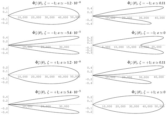
Figure 1. The normalized angular distributions ${\tilde{\Phi }}_i^{\pm }(\theta )$ in the polar coordinate system $(\tilde{\Phi },\theta )$ plotted for $k=1\mathrm{MeV}$, $\zeta =\pm 1$, $H={10}^4\mathrm{gauss}$, $E=1\mathrm{GeV}$, $\delta ={10}^{-3}$.

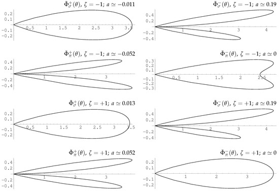
Figure 2. The normalized angular distributions ${\tilde{\Phi }}_i^{\pm }(\theta )$ in the polar coordinate system $(\tilde{\Phi },\theta )$ plotted for $k=0.25E$, $\zeta =\pm 1$, $H=0.1H_c$, $E=10m$, $\delta =0.1$.

3. Synchrotron Radiation in the Presence of a Stimulating Electromagnetic Wave

Recently, in connection with the more intense development of maser technology, much attention has been paid to stimulated electromagnetic emission. Therefore, it is interesting, besides the study of the interaction with a constant pseudovector field and with an anomalous vacuum magnetic moment, to calculate synchrotron radiation in the presence of a stimulating electromagnetic wave and accounting for the inhomogeneity of an external magnetic field (In this section, the velocity of light is written as c and the Plank constant as ℏ.). In this section, radiative transitions of relativistic electrons moving in a stationary, but inhomogeneous magnetic field are investigated in the presence of a stimulating electromagnetic wave. The regions of variation of the harmonics of the wave for which the stimulated radiation should exceed absorption is found.

3.1. The Electron Energy Spectrum

In this subsection, developing further the previous studies (see, e.g., [20] ), where similar emission in a constant and homogeneous magnetic field was investigated (for spontaneous emission in an inhomogeneous magnetic field, see, e.g., [26]) and in which, as is well known, no stability was obtained along the field direction, we considered stimulated emission by an electron placed in an axially symmetrical focusing magnetic field:

$$\mathbf{H}=H_z{\mathbf{e}}_z,H_z=H_0{r}^{-q},$$

where $r={(x^2+y^2)}^{1/2}$ and q is the field fall-off exponent, which in the case of stable motion, should lie in the range $0<q<1$. The energy spectrum of the electron is given, in the relativistic case (without accounting for the spin), by the expression:

$$E_{lsk}=E_l+\hslash {\omega }_l(\sqrt{1-q}s+\sqrt{q}k),$$

(57)

where

$$E_l=c\hslash {[{\gamma }^2(2-q)]}^2{R}^{2(1-q)}+{[k_0^2]}^{1/2},k_o=mc/\hslash ,$$

$${\omega }_l=\frac{eH(R)c}{E_l}=\frac{\beta c}{R},$$

$$\gamma =\frac{e{H}_0}{(2-q)c\hslash },R={[l/\gamma (1-q)]}^{1/(2-q)},$$

where R is the radius of the equilibrium orbit, $\omega$ is the frequency of revolution of the electron, and $l,s,$ and $k=0,1,2\cdots$ are, respectively, the orbital, radial, and axial quantum numbers.

3.2. Quantum Transitions

Let us consider the transitions $l,s,k\to l^{\prime }\ne l,s^{\prime }=s,k^{\prime }=k$, stimulated by an external field of frequency $\omega \approx (l-l^{\prime }){\omega }_l=\pm \nu {\omega }_l$, where $\nu >0$ is the number of the harmonic; in the case of light emission, $l-l^{\prime }=\nu$, while in the case of absorption, $l-l^{\prime }=-\nu$.

We assume that the external electromagnetic wave is linearly polarized and propagates at an angle $\theta$ to the direction of the magnetic field. In this case, the probability of the stimulated transition is given by the following formula (see, for example, [20]):

$$w_{l{l}^{\prime }}=\frac{2\pi N(\kappa )e_0^2{c}^4}{\hslash L^3\omega E_l{E}_l^{\prime }}{S}_i{g}_{l-l^{\prime }}(\omega ),i=x,z^{\prime }.$$

(58)

Here, $N(\kappa )$ is the number of photons with momentum $\kappa$ in the volume $L^3$, $\tau$ is the average lifetime of the electron in the initial state, and

$$g_{l-l^{\prime }}(\omega )=\frac{4\tau }{1+4{\tau }^2{({\omega }_{l{l}^{\prime }}-\omega )}^2},S_x=|P_x{|}^2,S_{z^{\prime }}={\left|P_y\right|}^2{cos}^2\theta .$$

The indices x and $z^{\prime }$ denote the polarization of the external wave: for the x component, the vector of the electric field $E_x$ lies in the plane of the electron orbit and is directed along the x-axis; for the $z^{\prime }$ component, the vector of the electric field $E_{z^{\prime }}$ is perpendicular to $E_x$ and to the propagation direction of the wave (i.e., it is almost parallel with the z-axis).

The matrix elements:

$$P_{x,y}=\int {\psi }_{l^{\prime },s,k}^{+}{e}^{-i\mathit{\kappa }\mathbf{r}}{\widehat{P}}_{x,y}{\psi }_{l,s,k}{d}^{3}x$$

are, assuming the amplitudes of the radial and axial oscillations to be small,

$$P_{x,y}=\frac{\hslash }{2R}\left\{\begin{array}{c}i{X}_{l,l_{\mp }\nu }(\theta ,\kappa )\hfill \\ Y_{l,l_{\mp }\nu }(\theta ,\kappa )\hfill \end{array}\right.,$$

(59)

where $\mathit{\kappa }=\kappa {\mathit{\kappa }}^0$ is the wave vector of the incident photon, and the quantities

$$X_{l,l\mp \nu }=-2l\frac{2-q}{1-q}{J}_{\nu }^{\prime }(\eta )\pm \frac{\nu ({\nu }^2-{\eta }^2-q)}{\eta (1-q)}{J}_{\nu }(\eta ),Y_{l,l\mp \nu }=\pm \frac{2l(2-q)\nu +{\eta }^2}{\eta (1-q)}{J}_{\nu }(\eta )-\frac{({\nu }^2-q)}{(1-q)}{J}_{\nu }^{\prime }(\eta )$$

(60)

are expressed in terms of the Bessel function $J_{\nu }$ and its derivative, which depends on the argument $\eta =\kappa Rsin\theta =\nu \beta sin\theta$.

The denominator in (58) is equal to

$$\frac{1}{E_l{E}_l^{\prime }}=\frac{1}{E_l^2}(1\pm {\beta }^2\frac{1-q}{2-q}\frac{\nu }{l}),$$

(61)

and for the factor $g_{l-l^{\prime }}(\omega )$, we have

$$g_{\nu }(\omega )=\frac{4\tau }{1+4{\tau }^2{({\omega }_{l,l+\nu }-\omega )}^2}=\frac{4\tau }{1+{\nu }^2{\delta }^2},$$

(62)

$$g_{-\nu }(\omega )=\frac{4\tau }{1+4{\tau }^2{({\omega }_{l,l-\nu }-\omega )}^2}=\frac{4\tau }{1+{\nu }^2{\delta }^2}$$

$$-16{\nu }^3{\tau }^2\delta {\beta }^2\omega (1-q+q{\beta }^{-2})\frac{1}{(2-q)l{(1+{\nu }^2{\delta }^2)}^2},$$

where $\delta =2\tau ({\omega }_{l,l+\nu }-\omega /\nu ).$

We now determine the power radiated by the electron in resonant transitions under the influence of an external electromagnetic wave, at the harmonic $\nu$:

$$W(\nu )=\hslash {\omega }_{l,l-\nu }{w}_{l,l-\nu }-\hslash {\omega }_{l,l+\nu }{w}_{l,l+\nu }.$$

(63)

Introducing the intensity of the electric field of the wave $\mathcal{E}$, connected with $N(\kappa )$ by the relation:

$${\mathcal{E}}^2/4\pi =\hslash \omega N(\kappa )/L^3,$$

we obtain the following expressions for the radiation power in the weakly relativistic limit (${\beta }^2>0$ and ${\beta }^4\approx 0$)—dipole radiation ($\nu =1$):

$$W=W_x+W_{z^{\prime }}=-\frac{e_0^2{\mathcal{E}}^2\tau }{m_0}\frac{1+{cos}^2\theta }{1+{\delta }^2}\frac{2-3q}{2(1-q)}+({\beta }^2+\frac{q}{1-q})\frac{2\delta \Omega \tau }{1+{\delta }^2},$$

(64)

where $\Omega =e_{0}H(R)/m_{0}c$. It then follows that, in an inhomogeneous field ($q\ne 1$), stimulated emission is possible ($W>0$) at the fundamental harmonic in the case of resonance ($\delta =0$) when $q>2/3$.

In the ultrarelativistic approximation ($\beta \to 1$), just as in the case of a homogeneous field (see [20]), we have a region of variation of the harmonics $\nu$ in which even stimulated emission can prevail over absorption ($W>0$) in the presence of resonance.

To find this region, let us consider first the case when the external electromagnetic wave has only an x component and is incident at an angle $\theta$ close to $\pi /2$, i.e., the wave vector lies near the plane of the electron orbit. Then,

$$sin\theta =1-{\alpha }^2/2(\alpha =\pi /2-\theta ),1-{\beta }^2\ll 1$$

and the following approximations of the Bessel functions in terms of the Macdonald functions $K_m$ hold:

$$J_{\nu }(\nu \beta sin\theta )=\frac{{(1-{\beta }^2{sin}^2\theta )}^{1/2}}{\pi \sqrt{3}}{K}_{1/3}(\frac{\nu }{3}{(1-{\beta }^2{sin}^2\theta )}^{1/2}),$$

$$J_{\nu }^{\prime }(\nu \beta sin\theta )=\frac{1-{\beta }^2{sin}^2\theta }{\pi \sqrt{3}}{K}_{2/3}(\frac{\nu }{3}{(1-{\beta }^2{sin}^2\theta )}^{1/2}).$$

(65)

If we assume that the argument of the functions $K_{1/3}$ and $K_{2/3}$ is small:

$$\frac{\nu }{3}{(1-{\beta }^2{sin}^2\theta )}^{1/2}\ll 1,$$

then it follows from (65) that

$$J_{\nu }(\eta )=\frac{\mathrm{\Gamma }(1/3)}{2^{2/3}{3}^{1/6}\pi {\nu }^{1/3}},J_{\nu }^{\prime }(\eta )=\frac{\mathrm{\Gamma }(2/3)3^{1/6}}{2^{1/3}\pi {\nu }^{2/3}},$$

(66)

and in the resonance case $\delta =0$, we obtain for the radiated power the expression:

$$W_x(\nu )=\frac{9^{2/3}{2}^{1/3}{\left[\mathrm{\Gamma }(2/3)\right]}^2{e}_0^2{c}^2{\epsilon }^2\tau }{{\pi }^2{\nu }^{4/3}{E}_l}$$

$$\times \{\frac{3-2q}{3(1-q)}-\frac{2^{5/3}\pi {\nu }^{4/3}(1-{\beta }^2+{\alpha }^2-q/{\nu }^2)}{3^{11/6}{\left[\mathrm{\Gamma }(2/3)\right]}^2(1-q)}\}.$$

(67)

We put here

$$1-{\beta }^2{sin}^2\theta \approx 1-{\beta }^2+{\alpha }^2.$$

The power $W_x$ will be positive (radiation) in two cases:

(1) If ${\alpha }^2<1-{\beta }^2$, then $\nu <{(1-{\beta }^2)}^{-3/4}=\sqrt{{\nu }_{max}}$ (${\nu }_{max}$ corresponds to the maximum of spontaneous emission);

(2) If ${\alpha }^2>1-{\beta }^2$, then $\nu <{\alpha }^{-3/2}$.

When one of these inequalities is violated, the system becomes absorbing, i.e., $W_x<0$. To increase the interval of harmonics in which the amplification of the radiation takes place, it is convenient to choose an angle $\alpha <\sqrt{1-{\beta }^2}=m_0{c}^2/E$.

For the $z^{\prime }$ component in the ultrarelativistic case, in the presence of resonance, only absorption will be observed ($W_{z^{\prime }}<0$), and this can be used, for example, for electron acceleration.

4. Electron in a Superposition of Electromagnetic Waves

4.1. Plane Wave

The Hamilton–Jacobi relativistic equation is:

$$\begin{array}{c}\hfill {\left(\frac{\partial S}{\partial x}+eA\right)}^2=m^2,\end{array}$$

(68)

where $c=1$. Consider a plane electromagnetic field with the vector potential:

$$A=A(\varphi ),\mathrm{where}\varphi =nx,n^2=0.$$

(69)

The following condition is applied to the potentials:

$$\partial A=(n\frac{dA}{d\varphi })=0,$$

(70)

which is equivalent to $(An)=0$. We seek a solution of Equation (68) in the form

$$\begin{array}{c}\hfill S=-(px)+F(\varphi ),p^{\mu }=\mathrm{const},p^2=m^2,\end{array}$$

(71)

where function F is to be found. We have $\frac{\partial S}{\partial x}=-p+F^{\prime }n$, and hence,

$${(\frac{\partial S}{\partial x}+eA)}^2=p^2+{(eA)}^2-2e(pA)-2(pn)F^{\prime }.$$

Equation (68) is transformed to

$$\begin{array}{c}\hfill {(eA)}^2-2e(pA)-2F^{\prime }(np)=0\end{array}$$

(72)

and its solution is as follows:

$$\begin{array}{c}\hfill F=\frac{1}{2(np)}\int d\varphi \left[{(eA)}^2-2e(pA)\right].\end{array}$$

(73)

Thus, the complete integral of the H-J equation results (sic):

$$\begin{array}{c}\hfill S=-(px)+F=-(px)+\frac{1}{2(np)}\int d\varphi \left[{(eA)}^2-2e(pA)\right].\end{array}$$

(74)

Here, $p^2=m^2$, and hence, we may choose independent components (We here use the metric (+ - - - ), $ab=a^0{b}^0-\mathbf{a}\mathbf{b}$, and again a system of units with $\hslash =c=1,\alpha =e^2=1/137$.):

$$(np)=p^0-p^1,\mathrm{and}\mathbf{p}=(p^2,p^3),$$

so that

$$(px)=p^0{x}^0-p^1{x}^1-\mathbf{pr}$$

and

$${(p)}^2={(p^0)}^2-{(p^1)}^2-{(\mathbf{p})}^2=(np)(p^0+p^1)-{(\mathbf{p})}^2=m^2,$$

and hence,

$$p^0+p^1=\frac{m^2+{\mathbf{p}}^2}{(np)},$$

$$\begin{array}{cc}\hfill px& =\frac{1}{2}(p^0+p^1)(x_0-x_1)+\frac{1}{2}(p^0-p^1)(x_0+x_1)-\mathbf{p}\mathbf{r}\hfill \\ \hfill & =\frac{1}{2}\frac{m^2+{\mathbf{p}}^2}{(np)}(x^0-x^1)+\frac{1}{2}(np)(x^0+x^1)-\mathbf{p}\mathbf{r}.\hfill \end{array}$$

(75)

According to the Jacobi theorem, in order to obtain the equations of motion, we have to put derivatives of S over constants $\mathbf{p}$ and $(np)$ equal to new constants, which we chose to be equal to zero (initial conditions) (In what follows, we chose a special reference frame, where $n=(1,1,0,0)$ and $\varphi =(nx)=(x^0-x^1)$.)

$$\begin{array}{cc}\hfill & \frac{\partial S}{\partial \mathbf{p}}=\frac{\partial }{\partial \mathbf{p}}(-(px)+\frac{1}{2(np)}\int d\varphi \left[{(eA)}^2-2e(pA)\right])\hfill \\ \hfill & =\mathbf{r}+\frac{e}{(np)}\int d\varphi \mathbf{A}-\frac{\mathbf{p}}{(np)}\varphi =0,,\hfill \end{array}$$

(76)

so that (sic)

$$\mathbf{r}=\frac{\mathbf{p}}{(np)}\varphi -\frac{e}{(np)}\int d\varphi \mathbf{A}.$$

(77)

Now, we find derivatives of S over $(np)$:

$$\begin{array}{cc}\hfill & \frac{\partial S}{\partial (np)}=-\int d\varphi \left[\frac{{(eA)}^2-2e(pA)}{2{(np)}^2}-\frac{m^2+{\mathbf{p}}^2}{2{(np)}^2}\right]\hfill \\ \hfill & -\frac{x^0+x^1}{2}=0,\hfill \end{array}$$

(78)

and hence, we find an equation for $x^1$ (sic):

$$x^1=\frac{1}{2}\left(\frac{m^2+{\mathbf{p}}^2}{{(np)}^2}-1\right)\varphi -\int d\varphi \frac{\left[{(eA)}^2-2e(pA)\right]}{2{(np)}^2},$$

(79)

where $\varphi$ is a parameter.

In what follows, we chose the gauge:

$$A_0=0,(\mathbf{n}\mathbf{A})=0,\mathrm{i}.\mathrm{e}.\mathbf{A}=(0,A_2,A_3).$$

(80)

Generalized momentum $\mathbf{p}=\mathbf{P}+e\mathbf{A}$ and energy $\epsilon$ are defined by differentiating the action with respect to coordinates and time, which gives

$$\begin{array}{c}{p}_2=P_2+e{A}_2,p_3=P_3+e{A}_3,\end{array}$$

i.e., for kinematic momentum, we have

$$\begin{array}{cc}\hfill P_2& =p_2-e{A}_2,P_3=p_3-e{A}_3,\hfill \\ \hfill P_1& =p_1=-\frac{(np)}{2}+\frac{m^2+{\mathbf{p}}^2}{2(np)}-\frac{e}{(np)}\mathbf{pA}+\frac{e^2}{2(np)}{\mathbf{A}}^2,\hfill \\ \hfill \epsilon & =(np)+P_1,\hfill \end{array}$$

(81)

which is in agreement with [10].

4.2. Bichromatic Wave

Consider a bichromatic wave $\mathbf{A}={\mathbf{A}}^{(1)}+{\mathbf{A}}^{(2)}$ as a superposition of two circularly polarized waves with frequencies ${\omega }_1$ and ${\omega }_2$ propagating in the direction $\mathbf{n}(|\mathbf{n}|=1)$, where

$$\begin{array}{c}{\mathbf{A}}^{(1)}=-\frac{E^{(1)}}{{\omega }_1}({\mathbf{e}}_{2}sin{\omega }_1\varphi -g_1{\mathbf{e}}_{3}cos{\omega }_1\varphi ),\\ {\mathbf{A}}^{(2)}=-\frac{E^{(2)}}{{\omega }_2}({\mathbf{e}}_{2}sin({\omega }_2\varphi +\alpha )-g_2{\mathbf{e}}_{3}cos({\omega }_2\varphi +\alpha )).\end{array}$$

Here, ${\mathbf{e}}_2,{\mathbf{e}}_3$ are unit vectors orthogonal to each other and to $\mathbf{n}\parallel \mathbf{Ox}$, $\varphi =t-(\mathbf{nr})=x^0-x^1$, and circular polarizations $g_1=\pm 1,g_2=\pm 1$.

Now,

$$S(\varphi )=-S_H(\varphi )+\mathbf{pr}-(np)x_0,$$

hence (sic),

$$\begin{array}{cc}\hfill S_H(\varphi )& =-S(\varphi )+\mathbf{pr}-(np)x_0\hfill \\ \hfill & =\frac{1}{2}\frac{m^2+{\mathbf{p}}^2}{(np)}(x^0-x^1)\hfill \\ \hfill & +\frac{1}{2}(np)(x^0+x^1)-\mathbf{p}\mathbf{r}+\mathbf{p}\mathbf{r}-(np)x_0\hfill \\ \hfill & -\frac{1}{2(np)}\int d\varphi \left[{(eA)}^2-2e(pA)\right]\hfill \\ \hfill & =\frac{1}{2}\frac{m^2+{\mathbf{p}}^2}{(np)}(x^0-x^1)-\frac{1}{2}(np)(x^0-x^1)\hfill \\ \hfill & -\frac{1}{2(np)}\int d\varphi \left[{(eA)}^2-2e(pA)\right],\hfill \end{array}$$

(82)

which is in agreement with the Herrmann formula [27] For this configuration, the action $S_H(\varphi )$, according to [27], can be found in the explicit form:

$$\begin{array}{c}\hfill S_H(\varphi )=\frac{1}{2(np)}\left[{\mathbf{p}}^2+m^2(1+{\gamma }^2)-{(np)}^2\right]\varphi \\ \hfill +\frac{e{E}^{(1)}}{(np){\omega }_1^2}(p_{2}cos{\omega }_1\varphi +g_1{p}_{3}sin{\omega }_1\varphi )\\ \hfill +\frac{e{E}^{(2)}}{(np){\omega }_2^2}(p_{2}cos({\omega }_2\varphi +\alpha )+g_2{p}_{3}sin({\omega }_2\varphi +\alpha ))\\ \hfill +g\frac{e^2{E}^{(1)}{E}^{(2)}}{(np){\omega }_1{\omega }_2}\frac{sin[({\omega }_1-g{\omega }_2)\varphi -g\alpha ]}{{\omega }_1-g{\omega }_2}.\end{array}$$

(83)

Here, $g=g_1{g}_2=\pm 1$ determines the relative polarization of waves, and

$$\gamma =\frac{e}{m}\sqrt{\overline{{\mathbf{A}}^2}}$$

(84)

with

$${\gamma }^2={\gamma }_1^2+{\gamma }_2^2,({\gamma }_i^2=\frac{e^2{E}^{(i)2}}{m^2{\omega }_i^2})$$

(85)

as the wave intensity parameter. One should note that the averaged value of ${\mathbf{A}}^2$ is

$$\overline{{\mathbf{A}}^2}=\overline{{({\mathbf{A}}^{(1)}+{\mathbf{A}}^{(2)})}^2}=\overline{{\mathbf{A}}^{(1)2}}+\overline{{\mathbf{A}}^{(2)2}}.$$

This classical solution (83) enters into a quantum solution of the Dirac equation [27].

4.3. Crossed Fields

Constant crossed fields may be considered as a special case of the field of a plane wave, if one takes a potential of the field as a particular form of the four-potential (69). Then, as a limiting case, we consider the crossed fields’ configuration $\mathbf{E}\perp \mathbf{H}$, $\left|\mathbf{E}\right|=\left|\mathbf{H}\right|=B$, given by the four-potential (see [10], p. 468):

$$A_{\mu }=(nx)a_{\mu },$$

(86)

so that, in our special frame, we have

$$\begin{array}{cc}\hfill a_{\mu }& =(0,0,B,0),\mathbf{n}\left|\right|Ox,(nx)=x^0-x^1=\varphi ,\hfill \\ \hfill \mathbf{E}& =-{\mathbf{A}}_{,t}=(0,-B,0),\mathbf{H}=\mathrm{rot}\mathbf{A}=(0,0,-\mathrm{B}).\hfill \end{array}$$

(87)

The solutions of Equations (77) and (79) can be written as

$$\mathbf{r}=\frac{\mathbf{p}}{(np)}\varphi -\frac{e}{(np)}\frac{{\varphi }^2}{2}\mathbf{B},$$

(88)

and

$$\begin{array}{cc}\hfill x^1& =\frac{1}{2}\left(\frac{m^2+{\mathbf{p}}^2}{{(np)}^2}-1\right)\varphi +\int d\varphi \frac{\left[{(eA)}^2-2e(pA)\right]}{2{(np)}^2}\hfill \\ \hfill & =\frac{1}{2}\left(\frac{m^2+{\mathbf{p}}^2}{{(np)}^2}-1\right)\varphi +\frac{1}{2{(np)}^2}\left[\frac{{\varphi }^3}{3}{e}^2{B}^2-e{\varphi }^2{p}_{2}B\right].\hfill \end{array}$$

(89)

Then, the following expression for the action (74) results:

$$\begin{array}{c}\hfill S=-(px)+F=-(px)+\frac{1}{2(np)}\left[\frac{{\varphi }^3}{3}{e}^2{B}^2-e{\varphi }^2{p}_{2}B\right].\end{array}$$

(90)

5. Radiation of a Charged Particle in a Superposition of Electromagnetic Waves

5.1. Radiation in the Field of a Plane Monochromatic Wave

According to [10], we have in general for the radiation power:

$$I=\frac{2e^4}{3m^2}\frac{{\left(\mathbf{E}+\mathbf{v}\times \mathbf{H}\right)}^2-{(\mathbf{E}\mathbf{v})}^2}{1-v^2}.$$

(91)

This problem was considered previously in [10] and also in [28]. We have for the monochromatic plane wave field according to Equation (80):

$$\begin{array}{cc}\hfill \mathbf{A}& =-\frac{E}{\omega }(0,sin\omega \varphi ,-gcos\omega \varphi ),\hfill \\ \hfill \mathbf{E}& =-{\mathbf{A}}_{,t}=E(0,cos\omega \varphi ,gsin\omega \varphi ),\hfill \\ \hfill \mathbf{H}& =E(0,-gsin\omega \varphi ,cos\omega \varphi ).\hfill \end{array}$$

(92)

For the kinematics, we have, according to (77),

$$\begin{array}{cc}\hfill \mathbf{r}& =\frac{\mathbf{p}}{(np)}\varphi -\frac{e}{(np)}\int d\varphi \mathbf{A},\hfill \\ \hfill \mathbf{v}& =\frac{d}{dt}\mathbf{r}=\frac{\mathbf{p}-e\mathbf{A}}{(np)}\hfill \\ \hfill & =\frac{1}{(np)}(0,p_2+e\frac{E}{\omega }sin\omega \varphi ,p_3-eg\frac{E}{\omega }cos\omega \varphi ).\hfill \end{array}$$

(93)

In the reference frame, where $\mathbf{p}=0$, we have the electric field $\mathbf{E}$ orthogonal to $\mathbf{v}$ and a magnetic field $\mathbf{H}$ parallel with v ($\mathbf{vE}=0$, $\mathbf{H}\times \mathbf{v}=0$). We also assume that the velocity along the x-axis, i.e., parallel with $\mathbf{n}$, is averaged to zero $p_1=0$ along with the initial condition $\mathbf{p}=0$ [10]. Then, we may use the known formula $\frac{m^2}{1-v^2}=p_1^2+{\mathbf{P}}^2+m^2$ to obtain

$$\frac{1}{1-v^2}=1+\frac{e^2{\mathbf{A}}^2}{m^2}.$$

(94)

We find the radiation power using the general formula (91), leading to

$$\begin{array}{cc}\hfill I& =\frac{2e^4}{3m^2}\frac{{\left(\mathbf{E}+\mathbf{v}\times \mathbf{H}\right)}^2-{(\mathbf{E}\mathbf{v})}^2}{1-v^2}\hfill \\ \hfill & =\frac{2e^4}{3m^2}\frac{{\mathbf{E}}^2}{1-v^2}=\frac{2e^4}{3m^2}{\mathbf{E}}^2\left(1+{(eE/m\omega )}^2\right).\hfill \end{array}$$

(95)

5.2. Radiation in the Field of a Plane Bichromatic Wave

We have:

$$\begin{array}{c}{\mathbf{A}}^{(1)}=-\frac{E^{(1)}}{{\omega }_1}({\mathbf{e}}_{2}sin{\omega }_1\varphi -g_1{\mathbf{e}}_{3}cos{\omega }_1\varphi ),\\ {\mathbf{A}}^{(2)}=-\frac{E^{(2)}}{{\omega }_2}({\mathbf{e}}_{2}sin({\omega }_2\varphi +\alpha )-g_2{\mathbf{e}}_{3}cos({\omega }_2\varphi +\alpha )).\end{array}$$

then the electric field:

$$\begin{array}{cc}\hfill {\mathbf{E}}^{(1)}& =E^{(1)}(0,cos{\omega }_1\varphi ,g_{1}sin{\omega }_1\varphi ),\hfill \\ \hfill {\mathbf{E}}^{(2)}& =E^{(2)}(0,cos({\omega }_2\varphi +\alpha ),g_{2}sin({\omega }_2\varphi +\alpha )),\hfill \end{array}$$

(96)

so that

$$\begin{array}{cc}\hfill \mathbf{E}& ={\mathbf{e}}_2(E^{(1)}cos{\omega }_1\varphi +E^{(2)}cos({\omega }_2\varphi +\alpha ))\hfill \\ \hfill & +{\mathbf{e}}_3(g_1{E}^{(1)}sin({\omega }_1\varphi )+g_2{E}^{(2)}sin({\omega }_2\varphi +\alpha ))\hfill \end{array}$$

(97)

and the magnetic field:

$$\begin{array}{cc}\hfill {\mathbf{H}}^{(1)}& =E^{(1)}(0,-g_{1}sin{\omega }_1\varphi ,cos{\omega }_1\varphi ),\hfill \\ \hfill {\mathbf{H}}^{(2)}& =E^{(2)}(0,-g_{2}sin({\omega }_2\varphi +\alpha ),cos({\omega }_2\varphi +\alpha )).\hfill \end{array}$$

(98)

For the kinematics, we have, as a generalization of (93),

$$\begin{array}{cc}\hfill \mathbf{v}& =\frac{1}{(np)}(0,p_2+e\frac{E^{(1)}}{{\omega }_1}sin{\omega }_1\varphi ,p_3-e{g}_1\frac{E^{(1)}}{{\omega }_1}cos{\omega }_1\varphi )\hfill \\ \hfill +& \frac{1}{(np)}(0,p_2+e\frac{E^{(2)}}{{\omega }_2}sin({\omega }_2\varphi +\alpha ),p_3-e{g}_2\frac{E^{(2)}}{{\omega }_2}cos({\omega }_2\varphi +\alpha )).\hfill \end{array}$$

(99)

Now, we use again the general expression (91) to find the radiation power. First, we have for the velocity:

$$\begin{array}{cc}\hfill \mathbf{v}& =\frac{e{E}^{(1)}}{(np){\omega }_1}(0,sin{\omega }_1\varphi ,-g_{1}cos{\omega }_1\varphi )\hfill \\ \hfill +& \frac{e{E}^{(2)}}{(np){\omega }_2}(0,sin({\omega }_2\varphi +\alpha ),-g_{2}cos({\omega }_2\varphi +\alpha ))\hfill \\ \hfill & ={\mathbf{e}}_{\mathbf{2}}\left[\frac{e{E}^{(1)}}{(np){\omega }_1}sin{\omega }_1\varphi +\frac{e{E}^{(2)}}{(np){\omega }_2}sin({\omega }_2\varphi +\alpha )\right]\hfill \\ \hfill & +{\mathbf{e}}_{\mathbf{3}}\left[-g_1\frac{e{E}^{(1)}}{(np){\omega }_1}cos{\omega }_1\varphi -g_2\frac{e{E}^{(2)}}{(np){\omega }_2}cos({\omega }_2\varphi +\alpha )\right].\hfill \end{array}$$

(100)

According to (81), in the reference frame where the particle is at rest on average, we have

$$\begin{array}{cc}\hfill P_2& =-e{A}_2,P_3=-e{A}_3,\hfill \\ \hfill P_1& =p_1=0,\epsilon =(np).\hfill \end{array}$$

(101)

We also assume that the velocity along the x-axis, i.e., parallel with $\mathbf{n}$, is averaged to zero $p_1=0$ along with the initial condition $\mathbf{p}=0$ [10]. Now, we can obtain the following:

$$\begin{array}{cc}\hfill & {\left(\mathbf{E}+\mathbf{v}\times \mathbf{H}\right)}^2-{(\mathbf{E}\mathbf{v})}^2\hfill \\ \hfill & ={\mathbf{E}}^2+2\mathbf{E}[\mathbf{v}\times \mathbf{H}]+{[\mathbf{v}\times \mathbf{H}]}^2-{(\mathbf{E}\mathbf{v})}^2={\mathbf{E}}^2.\hfill \end{array}$$

(102)

Indeed, we have $\mathbf{E}[\mathbf{v}\times \mathbf{H}]=\mathbf{v}[\mathbf{H}\times \mathbf{E}]=0$, since $\mathbf{v}$ lies in the $yz$ plane. Moreover,

$${(\mathbf{E}\mathbf{v})}^2={([\mathbf{H}\times \mathbf{n}]\mathbf{v})}^2={([\mathbf{v}\times \mathbf{H}]\mathbf{n})}^2={[\mathbf{v}\times \mathbf{H}]}^2.$$

Finally, with the help of Equations (94) and (91), we obtain the radiation power in a bichromatic wave:

$$\begin{array}{cc}\hfill I& =\frac{2e^4}{3m^2}\frac{{\left(\mathbf{E}+\mathbf{v}\times \mathbf{H}\right)}^2-{(\mathbf{E}\mathbf{v})}^2}{1-v^2}\hfill \\ \hfill & =\frac{2e^4}{3m^2}\frac{{\mathbf{E}}^2}{1-v^2}=\frac{2e^4}{3m^2}{\mathbf{E}}^2\left(1+{\gamma }^2\right),\hfill \end{array}$$

(103)

with ${\gamma }^2$ defined in Equations (84) and (85).

5.3. Radiation in Crossed Fields

Let $\mathbf{E}$ and $\mathbf{H}$ be crossed fields (87), then we have ($\mathcal{E}=p_0$):

$$\begin{array}{cc}\hfill I& =\frac{2e^4{B}^2}{3m^2}\frac{{(1-v_1)}^2}{1-v^2}=\frac{2e^4{B}^2}{3m^4}{\mathcal{E}}^2{(1-v_1)}^2\hfill \\ \hfill & =\frac{2e^4{B}^2}{3m^4}{(p_0-p_1)}^2.\hfill \end{array}$$

(104)

This expression is in full agreement with the formula from Nikishov and Ritus [29] (p. 534).

6. Discussion

The calculation of the angular distribution (e.g., [23,24]) was made in the framework of the Standard Model. In this paper, we made our calculations accounting for the SME technique and employed the standard methods of QED. Our results were based on exact solutions of the Dirac equation for an electron with a vacuum magnetic moment in a constant magnetic field. They were due to the specific non-perturbative interaction of the electron vacuum magnetic moment $\mu$ with the condensate, violating Lorentz invariance. In our work, we considered the radiation phenomena in the entirely quantum approach and obtained the asymptotic expressions for the spectral–angular distribution for the case of a high-energy particle moving in a relatively weak magnetic field; these expressions include all the quantum corrections in our problem.

It was also mentioned that there exists a way to use corresponding semiclassical solutions to the Dirac equation themselves to consider synchrotron radiation in a nonuniform magnetic field instead of using it for the radiative amplitudes, which may help to consider radiation in more realistic conditions.

We calculated the stimulated radiation of SR in a nonuniform magnetic field regardless of the spin variables of the electron. The conditions for the amplification of the radiation were found.

It can be demonstrated that there is a way to use a corresponding semiclassical solution to the Dirac equation to consider synchrotron radiation without approximating (as was done, for instance, in ([20] and in the text above (42)) the radiative amplitudes, but finding the approximation for the electron wave functions themselves. In this way, in a magnetic field $\mathbf{H}=H{\mathbf{e}}_z$, $H>0$, with the vector potential $A_0=0,\mathbf{A}=(0,xH,0)$, one can use Airy functions for approximating the electron wave function in trajectory

$$\Phi (-x_{1,2})=\frac{1}{2\sqrt{\pi }}{\int }_{-\infty }^{+\infty }dtexp(-i{x}_{1,2}t+i{t}^3/3),$$

where

$$x_{1,2}={(2eH{p}_{\perp })}^{1/3}(x\mp 1/2p_{\perp })),$$

and

$$p_{\perp }=\sqrt{E^2-m^2-p^2}.$$

This last way of calculation with approximating the electron wave function only on a short part of its trajectory might be of use for studying SR in real circumstances of radiation in an astrophysical magnetic field and in a nonuniform magnetic field, where the electron trajectories are far from being circular.

7. Conclusions

The form of the Lorentz symmetry breaking we considered in this paper is only one of the possible types of SM violations. The results of our work may give us one possible way to detect a violation of Lorentz invariance. The form of other types of external influences we considered in this paper, such as a superposition of two electromagnetic waves or crossed fields, are just possible types of external influences that should be taken into account in experiments with electrons in external fields. For instance, the consideration of the stimulating influence of an external electromagnetic wave on SR in a nonuniform magnetic field may find some application in using lasers in the studies of the SR in accelerators. It was also mentioned that there exists a way to use corresponding semiclassical solutions to the Dirac equations themselves to consider synchrotron radiation in a nonuniform magnetic field instead of using it for the radiative amplitudes, which may help to consider radiation in more realistic conditions. This may be considered in our forthcoming publications.

References

- Colladay, D.; Kostelecký, V.A. CPT violation and the standard model. Phys. Rev. D 1997, 55, 6760. [Google Scholar] [CrossRef]
- Colladay, D.; Kostelecký, V.A. Lorentz-violating extension of the standard model. Phys. Rev. D 1998, 58, 116002. [Google Scholar] [CrossRef]
- Kostelecký, V.A.; Lane, C. Nonrelativistic quantum Hamiltonian for Lorentz violation. J. Math. Phys. 1999, 40, 6245. [Google Scholar] [CrossRef]
- Kostelecký, V.A.; Lane, C. Constraints on Lorentz violation from clock-comparison experiments. Phys. Rev. D 1999, 60, 116010. [Google Scholar] [CrossRef]
- Bluhm, R.; Kostelecký, V.A.; Lane, C.D.; Russell, N. Probing Lorentz and CPT violation with space-based experiments. Phys. Rev. D 2003, 68, 125008. [Google Scholar] [CrossRef]
- Bluhm, R. Overview of the Standard Model Extension: Implications and Phenomenology of Lorentz Violation. arXiv 2005, arXiv:hep-ph/05060549. [Google Scholar]
- Mattingly, D. Modern Tests of Lorentz Invariance. Living Rev. Rel. 2005, 8, 5. [Google Scholar] [CrossRef]
- Zhukovsky, V.C.; Frolov, I.E. Synchrotron Radiation Under Conditions of Violated Lorentz Invariance. Mosc. Univ. Phys. Bull. 2008, 63, 10. [Google Scholar]
- Frolov, I.E.; Zhukovsky, V.C. Synchrotron radiation in the standard model extension. J. Phys. A Math. Theor. 2007, 40, 10625. [Google Scholar] [CrossRef]
- Berestetskii, V.B.; Lifshitz, E.M.; Pitaevskii, L.P. Quantum Electrodynamics; Pergamon: Oxford, UK, 1982. [Google Scholar]
- Pauli, W. Relativistic Field Theories of Elementary Particles. Rev. Mod. Phys. 1941, 13, 203. [Google Scholar] [CrossRef]
- Schwinger, J. On Quantum-Electrodynamics and the Magnetic Moment of the Electron. Phys. Rev. 1948, 73, 416. [Google Scholar] [CrossRef]
- Zhukovsky, V.C.; Lobanov, A.E.; Murchikova, E.M. Radiative effects in the standard model extension. Phys. Rev. D 2006, 73, 065016. [Google Scholar] [CrossRef]
- Andrianov, A.A.; Giacconi, P.; Soldati, R. Spontaneous CPT asymmetry of the Universe. Grav. Cosmol. Suppl. 2002, 8N1, 41. [Google Scholar]
- Borisov, A.V.; Goryaga, O.G.; Zhukovsky, V.C.; Sokolov, A.A. Pair creation on a nucleus in a field of bichromatic electromagnetic wave. Izv. Vuz. Fiz. 1978, 9, 33–40. [Google Scholar]
- Flouris, K.; Jimenez, M.M.; Debus, J.-D.; Herrmann, H.J. Confining massless Dirac particles in two-dimensional curved space. Phys. Rev. B 2018, 98, 155419. [Google Scholar] [CrossRef]
- Flouris, K.; Jimenez, M.M.; Herrmann, H.J. Curvature-induced quantum spin-Hall effect on a Möbius strip. Phys. Rev. B 2022, 105, 235122. [Google Scholar] [CrossRef]
- Pi, T.-W.; Hong, I.-H.; Cheng, C.-P. Synchrotron-radiation photoemission study of Ba on W(110). Phys. Rev. B 1998, 58, 4149. [Google Scholar] [CrossRef]
- Ternov, I.M.; Bagrov, V.G.; Zhukovsky, V.C. Synchrotron radiation of an electron with a vacuum magnetic moment. Vestnik Mosk. Univ. Fiz. Astron. 1966, 7, 30. [Google Scholar]
- Sokolov, A.A.; Ternov, I.M. Radiation from Relativistic Electrons; American Institute of Physics: New York, NY, USA, 1986. [Google Scholar]
- Bordovitsyn, V.A. (Ed.) Synchrotron Radiation Theory and its Development: In Memory of I. M. Ternov; Series on Synchrotron Radiation Techniques and Application; World Scientific: Singapore, 1999; Volume 5. [Google Scholar]
- Altschul, B. Synchrotron and inverse Compton constraints on Lorentz violations for electrons. Phys. Rev. D 2006, 74, 083003. [Google Scholar] [CrossRef]
- Montemayor, R.; Urrutia, L.F. Synchrotron radiation in Lorentz-violating electrodynamics. Phys. Rev. D 2005, 72, 045018. [Google Scholar] [CrossRef]
- Ellis, J.; Mavromatos, N.E.; Sakharov, A.S. Synchrotron radiation from the Crab Nebula discriminates between models of space-time foam. Astropart. Phys. 2004, 20, 669. [Google Scholar] [CrossRef]
- Schwinger, J. The quantum correction in the radiation by energetic accelerated electrons. Proc. Nat. Acad. Sci. USA 1954, 40, 132. [Google Scholar] [CrossRef]
- Kholomai, B.V.; Zhukovskii, V.C. Electron radiation in a focusing magnetic field allowing for spin states. Vestn. Mosk. Univ. Ser. III Fiz. Astron. 1972, 13, 66. [Google Scholar]
- Zhukovsky, V.C.; Herrmann, I. Radiation of electron in the field of two electromagnetic waves. Mosc. Univ. Phys. Bull. 1970, 6, 671. [Google Scholar]
- Ternov, I.M.; Bagrov, V.G.; Khapaev, A.M. Radiation of a relativistic charge in a plane wave electromagnetic field. Annalen der Physik 1968, 477, 25. [Google Scholar] [CrossRef]
- Nikishov, A.I.; Ritus, V.I. Quantum processes in the field of a plane electromagnetic wave and in a constant field. Soviet Phys. JETP 1964, 19, 529. [Google Scholar]
Publisher’s Note: MDPI stays neutral with regard to jurisdictional claims in published maps and institutional affiliations. |
© 2022 by the author. Licensee MDPI, Basel, Switzerland. This article is an open access article distributed under the terms and conditions of the Creative Commons Attribution (CC BY) license (https://creativecommons.org/licenses/by/4.0/).