Axial Symmetric Granular Flow Due to Gravity in a Circular Pipe

Abstract

Axisymmetric granular flows in vertical cylindrical pipes under action of gravity are studied using mathematical particle–particle models based on the Hertz–Mindlin theory. By and large, in granular flows, the density field and the pressure are unknown scalar functions. A well-known relationship between these fields gives the pressure field a power law of the density. The aim of this paper was to study unsteady, axisymmetric, fully developed granular flow under gravity action in a vertical cylindrical pipe, under the assumptions that the density field is constant and the velocity on the pipe’s wall is time-dependent. Using integral transforms method and appropriate initial-boundary conditions, the analytical solution for axial velocity is determined. The obtained analytical solution is used to determine the steady-state solution (the solution for large values of the time). The properties of the flow in some particular cases of the velocity on the pipe’s surface are analyzed and the transient flow is compared with the stationary one.

1. Introduction

Granular materials are made up of a collection of individual macroscopic particles that interact with each other. Desert/beach sand and snow are well-known examples of granular materials. Granular flows behave as fluid flows under certain regimes, but their behavior differs from fluid ones [1].

Practical applications of granular flows are typical in agriculture, geophysics, pharmaceutics, the food sector, etc. Experimental or numerical simulations of granular flows are useful to predict natural phenomena such as landslides or avalanches. The transportation of grain or solid materials in powder through channels and narrow passages are other important applications of granular flows [2,3,4].

Williams [5] carried out a quantitative analysis of gravity-driven granular flows by using video software and compared results of their experiments with other existing in the literature. In the Williams experiment, the author highlighted the three possible flow regimes when a granular material falls downwards through the pipe. Depending on the ratio of the diameter of the pipe to the size of the particles, the flow can be free-fall, highly compact, or with density waves. Granular flows in vertical pipes that feed a chute with a converging outlet at the bottom to control the mass flux have been investigated by Barker et al. [6] using discrete element method. Farin et al. [7] conducted granular column collapse experiments on a flat rough surface tilted at various angles with synchronous measurements of the flow dynamics and the emitted seismic signal. They found that the ratio of radiated seismic energy to potential energy lost by the granular flows is slightly decreasing.

Ligneau et al. [8] developed a mathematical model of granular avalanches on a periodic inclined plane, using the distinct element method to explain how inter-particle cohesion and ground friction influences avalanche velocity. The cohesion between particles is modeled through bonds that can break/form representing fragmentation/aggregation potentials. Their model shows a good ability to reproduce the various flow regimes as observed in nature: for low cohesion, highly sheared and fast flows are obtained while slow plugs form above a critical cohesion value and for lower ground frictions. A depth-averaged model for granular flow facing obstacles on steep terrains has been studied by Yang et al. [9]. The authors used a second-order Riemann-free scheme to study the depth-averaged model with a wetting–drying technique. They carried out numerical simulations for the granular flow by considering a single hemispherical obstacle and system of three hemispherical obstacles. Their findings provide some supplemental understanding of flow structures of fast granular flow facing obstacles. Fazelpour and Daniels [10] have performed experiments in a quasi-bidimensional annular shear cell subject to different boundaries with controlled roughness/compliance. Using the photoelastic techniques, the authors measured the stress fields throughout the material. They observed that boundary roughness and compliance strongly control the profiles of velocity, shear stress, pressure, and shear rate. The macroscopic dynamic behavior of granular flow in a cylindrical hopper with flat bottom has been investigated by Zhu and Yu [11], using an averaging technique. The velocity, shear stresses, couple stresses, and density were illustrated to compare qualitatively the experimental and numerical results and confirm the validity of the proposed averaging method.

Blackmore et al. [12] formulated a new mathematical model based on a class of integro-partial differential equation for the prediction of granular flow dynamics. Their models are obtained using a novel limiting averaging method on the Newtonian equations of motion of a many-particle system incorporating inelastic particle–particle forces. In an approximate form, the models’ equations can be written as a system of partial differential equations of the Navier–Stokes type. The authors have obtained steady solutions of the new models for granular flows down on inclined planes and in vibrating beds. Other interesting topics related to granular flow have been studied in the references [13,14,15,16,17,18,19].

In this paper, we investigate a particular case of the unsteady granular flows described by the particle-particle models developed by Blackmore et al. [12] in the Hertz–Mindlin theory [20,21]. We determine exact analytical solutions for the unsteady, axisymmetric, fully developed granular flow under the gravity action in a vertical cylindrical pipe under the assumptions that the density field is constant and the velocity on the pipe’s wall is time-dependent.

Generally, the density field and the pressure are unknown scalar functions. The relationship between these fields is [12] $p=a{\rho }^b$, where $a>0, b>0$ are constants characteristic of the granular flow medium. Of course, the model studied in this article is found in particular cases of granular flows. We sought to numerically study a nonlinear model, and we believe that the solutions obtained in this particular case will be useful for validating the numerical solutions at least in cases where the density is an almost constant function.

In this study, we consider that the velocity of the particles in contact with the pipe wall is dependent on time. Using integral transforms method, the analytical solution for axial velocity is determined by two different ways, namely by using Laplace transform coupled with the residues theory in complex functions, respectively, the finite Hankel transform and Bessel functions.

The general analytical solution of the axial velocity is used to determine the steady-state solution (the solution for large values of the time). Note that the stationary solution obtained by us is identical to the one determined in ([12], Equation (31)) for the same type of movement but with constant speed on the pipeline’s surface.

To study the characteristics of the flow, numerical simulations were made using the Mathcad 14.0 software. The obtained results are represented graphically and discussed. The properties of the flow in some particular cases of the velocity on the pipe’s surface are analyzed and the transient flow is compared with the stationary one.

2. Statement of the Problem

Consider the transient granular flow under the action of gravity in a vertical circular cylinder of radius $R>0$ (Figure 1). The basic equations of granular flow are given by [12].

The continuity equation,

$$\frac{\partial \rho }{\partial t}+div(\rho v)=0,$$

(1)

and the momentum balance of the granular flow,

$$\frac{\partial \mathbf{v}}{\partial t}+(\mathbf{v}\cdot \nabla )\mathbf{v}=-g{\mathbf{e}}_z+\frac{1}{\rho }gradp+v\Delta v+\lambda grad(div v),$$

(2)

where $\rho$ is the density field, $p$ is the pressure, $g$ is the gravitational acceleration, $\mathbf{v}$ is the vector velocity field, and $\nu$ and $\lambda$ are material coefficients that may be assumed to be constants in many applications [12]. By and large, the pressure $p$ and the density $\rho$ are unknown functions; therefore, Equations (1) and (2) are insufficient to determine the velocity vector field $\mathbf{v}$ and scalar fields $p$ and $\rho$. By appending the energy equation to the continuity Equation (1) and the motion Equation (2), a relationship between the density and the pressure has been established.

The equation of state of granular flow medium is [12]

$$p=a{\rho }^b, a>0, b>0.$$

(3)

In this study, the cylindrical coordinate system $(r,\theta ,z)$, with the unit vectors ${\mathbf{e}}_r, {\mathbf{e}}_{\theta }, {\mathbf{e}}_z$ will be used.

The flow domain is $\Omega =\{A(r,\theta ,z)\in {ℝ}^3|0\le r\le R, 0\le \theta <2\pi , -\infty <z<\infty \}$ whose boundary $\partial \Omega =\{A(r,\theta ,z)\in {ℝ}^3|r=R, 0\le \theta <2\pi , -\infty <z<\infty \}$ is assumed to be rigid and impenetrable. In the following, the density field and pressure are assumed to be constant.

Denoting the velocity components by $(u_r,u_{\theta },u_z)$, where $u_r$ is the radial velocity, $u_{\theta }$ is the azimuthal velocity, and $u_z$ is the axial velocity, from Equation (1), and Equation (2) we obtain the scalar basic partial differential equations:

$$\frac{1}{r}\frac{\partial (r{u}_r)}{\partial r}+\frac{1}{r}\frac{\partial u_{\theta }}{\partial \theta }+\frac{\partial u_z}{\partial z}=0$$

(4)

$$\begin{array}{l}\frac{\partial u_r}{\partial t}+u_r\frac{\partial u_r}{\partial r}+\frac{u_{\theta }}{r}\frac{\partial u_r}{\partial \theta }+u_z\frac{\partial u_r}{\partial z}-\frac{u_{\theta }^2}{r}=\\ v\left[\frac{1}{r}\frac{\partial }{\partial r}\left(r\frac{\partial u_r}{\partial r}\right)+\frac{1}{r^2}\frac{{\partial }^2{u}_r}{\partial {\theta }^2}+\frac{{\partial }^2{u}_r}{\partial z^2}\right]+\lambda \frac{\partial }{\partial r}\left[\frac{1}{r}\frac{\partial (r{u}_r)}{\partial r}+\frac{1}{r}\frac{\partial u_{\theta }}{\partial \theta }+\frac{\partial u_z}{\partial z}\right],\end{array}$$

(5)

$$\begin{array}{l}\frac{\partial u_{\theta }}{\partial t}+u_r\frac{\partial u_{\theta }}{\partial r}+\frac{u_{\theta }}{r}\frac{\partial u_{\theta }}{\partial \theta }+u_z\frac{\partial u_{\theta }}{\partial z}+\frac{u_r{u}_{\theta }}{r}=\\ v\left[\frac{1}{r}\frac{\partial }{\partial r}\left(r\frac{\partial u_{\theta }}{\partial r}\right)+\frac{1}{r^2}\frac{{\partial }^2{u}_{\theta }}{\partial {\theta }^2}+\frac{{\partial }^2{u}_{\theta }}{\partial z^2}\right]+\frac{\lambda }{r}\frac{\partial }{\partial \theta }\left[\frac{1}{r}\frac{\partial (r{u}_r)}{\partial r}+\frac{1}{r}\frac{\partial u_{\theta }}{\partial \theta }+\frac{\partial u_z}{\partial z}\right],\end{array}$$

(6)

$$\begin{array}{l}\frac{\partial u_z}{\partial t}+u_r\frac{\partial u_z}{\partial r}+\frac{u_{\theta }}{r}\frac{\partial u_z}{\partial \theta }+u_z\frac{\partial u_z}{\partial z}=\\ -g+v\left[\frac{1}{r}\frac{\partial }{\partial r}\left(r\frac{\partial u_z}{\partial r}\right)+\frac{1}{r^2}\frac{{\partial }^2{u}_z}{\partial {\theta }^2}+\frac{{\partial }^2{u}_z}{\partial z^2}\right]+\lambda \frac{\partial }{\partial z}\left[\frac{1}{r}\frac{\partial (r{u}_r)}{\partial r}+\frac{1}{r}\frac{\partial u_{\theta }}{\partial \theta }+\frac{\partial u_z}{\partial z}\right].\end{array}$$

(7)

There are many practical problems in which the radial and azimuthal velocities have negligible values. In such problems, the axial velocity characterizes the granular flow. In this article, we study such a case, namely we seek to determine the velocity field in the form $\mathbf{v}(u_r=0, u_{\theta }=0, u_z=w(r,t))$. For considered velocity field, Equations (4)–(6) are trivially satisfied and the Equation (7) yields

$$\frac{\partial w(r,t)}{\partial t}=-g+\nu \frac{1}{r}\frac{\partial }{\partial r}\left(r\frac{\partial w(r,t)}{\partial r}\right)$$

(8)

Along with Equation (8), we consider the initial and boundary conditions as follows:

$$w(r,0)=0, r\in [0,R],$$

(9)

$$w(R,t)=-w_0{f}_1(t), w_0>0, t\ge 0,$$

(10)

where $f_1(t)$ is a differentiable function of the exponential order to infinity, $f_1(0)=0$, and $\underset{t\to \infty }{\lim }{f}_1(t)=1$.

Using following non dimensionless parameters,

$$\tilde{r}=\frac{r}{R}, \tilde{t}=\frac{\nu t}{R^2}, \tilde{w}=\frac{w}{w_0}, a_0=\frac{g{R}^2}{\nu w_0}, \tilde{f}(\tilde{t})=f_1\left(\frac{R^{2}t}{\nu }\right),$$

(11)

Equations (8)–(10) become

$$\frac{\partial \tilde{w}}{\partial \tilde{t}}=-a_0+\frac{1}{\tilde{r}}\left[\frac{\partial }{\partial \tilde{r}}\left(\tilde{r}\frac{\partial \tilde{w}}{\partial \tilde{r}}\right)\right],$$

(12)

$$\tilde{w}(\tilde{r},0)=0, \tilde{r}\in [0,1],$$

(13)

$$\tilde{w}(1,\tilde{t})=-\tilde{f}(\tilde{t}), \tilde{t}\ge 0.$$

(14)

For simplicity, in the next sections, the swung dash notation will be eliminated.

3. Solution of the Initial-Boundary Value Problem

In this section, we determine the analytical solution for the velocity field $w(r,t)$ in two different ways using the integral transforms method. In such manner, we will have a validation of the obtained analytical solution.

3.1. Method of Laplace Transform

Applying the Laplace transform [22,23] to Equation (12) and using the initial condition (13), we obtain the transformed equation as

$$\frac{a_0}{s}=-s\widehat{w}(r,s)+\frac{1}{r}\left[\frac{\partial }{\partial r}\left(r\frac{\partial \widehat{w}(r,s)}{\partial r}\right)\right],$$

(15)

where $\widehat{w}(r,s)={\displaystyle \underset{0}{\overset{\infty }{\int }}w(r,t)e^{-st}dt}$ denotes the Laplace transform of function $w(r,t)$, $s$ being the transform parameter. The function $\widehat{w}(r,s)$ has to satisfy the boundary condition

$$\widehat{w}(1,s)=-\widehat{f}(s)$$

(16)

It is easy to see that the function

$${\widehat{w}}_p(r,s)=-\frac{a_0}{s^2}$$

(17)

is a particular solution of Equation (15).

The homogenous equation associated to Equation (15) is

$$\frac{1}{r}\left[\frac{\partial }{\partial r}\left(r\frac{\partial \widehat{w}(r,s)}{\partial r}\right)\right]-s\widehat{w}(r,s)=0,$$

(18)

that can be written in the equivalent form

$$r^2\frac{{\partial }^2\widehat{w}}{\partial r^2}+r\frac{\partial \widehat{w}}{\partial r}-{\left(r\sqrt{s}\right)}^2\widehat{w}=0.$$

(19)

The Equation (19) is a modified Bessel equation, whose general solution is written as [24]

$${\widehat{w}}_{{}_h}(r,s)=A(s)I_0(r\sqrt{s})+B(s)K_0(r\sqrt{s}),$$

(20)

where $I_0(z)$ and $K_0(z)$ are Bessel functions of first and second kind and of zero order.

Since $\underset{z\to 0^{+}}{\lim }{K}_0(z)=+\infty$, then the solution will be regular at $r=0$ if $B(s)=0$. The general solution of Equation (15) is given by

$$\widehat{w}(r,s)={\widehat{w}}_h(r,s)+{\widehat{w}}_p(r,s)$$

(21)

Imposing the boundary condition (17), we find the solution of the velocity field in Laplace domain as

$$\widehat{w}(r,s)=-\frac{a_0}{s^2}+\left(\frac{a_0}{s^2}-\widehat{f}(s)\right)\frac{I_0(r\sqrt{s})}{I_0(\sqrt{s})}$$

(22)

The inverse Laplace transform of the function (22) will be determined using the residue theorem from the theory of complex functions [25]. To do this, we consider the auxiliary function,

$$\widehat{G}(r,s)=\frac{I_0(r\sqrt{s})}{I_0(\sqrt{s})}=\frac{J_0(ir\sqrt{s})}{J_0(i\sqrt{s})}$$

(23)

where $i$ is the complex unit.

Let us denote by $r_n, n=1, 2, 3,\dots$, the positive roots of the equation $J_0(z)=0$ [26]. The poles of function $\widehat{G}(r,s)$ are $s_n=-{\overline{r}}_n{}^2, n=1,2,3,\dots$.

By using the residue theorem, the inverse Laplace transform of the function $\widehat{G}(r,s)$ is

$$\begin{array}{l}G(r,t)={\displaystyle \sum _{n=1}^{\infty }Res(\widehat{G}(r,s),s=s_n)\exp (s_{n}t)}\\ ={\displaystyle \sum _{n=1}^{\infty }\exp (s_{n}t)}\underset{s\to s_n}{\lim }\frac{J_0(ir\sqrt{s})}{\frac{d}{ds}(J_0(i\sqrt{s}))}\\ ={\displaystyle \sum _{n=1}^{\infty }\exp (s_{n}t)}\underset{s\to s_n}{\lim }\frac{2i\sqrt{s} J_0(ir\sqrt{s})}{J_1(i\sqrt{s})}=2{\displaystyle \sum _{n=1}^{\infty }\frac{r_n{J}_0(r r_n)}{J_1(r_n)}\exp (-r_n^{2}t).}\end{array}$$

(24)

By applying the inverse Laplace transform on Equation (22) and using the properties of the Laplace transform, we obtain the velocity field $w(r,t)$ as

$$w(r,t)=-a_{0}t+a_{0}t\ast G(r,t)-f(t)\ast G(r,t),$$

(25)

where notation “$\ast$” denotes the convolution product.

A direct calculation shows that

$$\begin{array}{l}{a}_{0}t\ast G(r,t)=2a_0{\displaystyle \underset{0}{\overset{t}{\int }}(t-\tau ){\displaystyle \sum _{n=1}^{\infty }{r}_n\frac{J_0(r{r}_n)}{J_1(r_n)}{e}^{-{\overline{r}}^2{}_n\tau }d\tau }}=2a_{0}t{\displaystyle \sum _{n=1}^{\infty }\frac{J_0(r{r}_n)}{r_n{J}_1(r_n)}}\\ +2a_0{\displaystyle \sum _{n=1}^{\infty }\frac{r_n(1-e^{-r^2{}_{n}t})}{r^3{}_n}\frac{J_0(r{r}_n)}{J_1(r_n)}}\end{array},$$

(26)

Using the formula $2{\displaystyle \sum _{n=1}^{\infty }\frac{J_0(r{r}_n)}{r_n{J}_1(r_n)}=1, r\in [0,1)}$ [14] in the above equation, we obtain

$$a_{0}t\ast G(r,t)=a_{0}t+2a_0{\displaystyle \sum _{n=1}^{\infty }\frac{(e^{-r_n^{2}t}-1)}{r_n^3}\frac{J_0(r{r}_n)}{J_1(r_n)}}.$$

(27)

The last term in Equation (24) can be written as

$$\begin{array}{l}f(t)\ast G(r,t)=2{\displaystyle \sum _{n=1}^{\infty }\frac{r_n{J}_0(r{r}_n)}{J_1(r_n)}}{\displaystyle \underset{0}{\overset{t}{\int }}f(\tau )e^{-r_n{}^2(t-\tau )}d\tau }=\\ 2{\displaystyle \sum _{n=1}^{\infty }\frac{r_n{J}_0(r{r}_n)}{J_1(r_n)}}\left[\frac{1}{r_n^2}f(t)-\frac{1}{r_n^2}{\displaystyle \underset{0}{\overset{t}{\int }}{f}^{\prime }(\tau )}{e}^{-r_n{}^2(t-\tau )}d\tau \right]\\ =f(t)-2{\displaystyle \sum _{n=1}^{\infty }\frac{J_0(r{r}_n)}{r_n{J}_1(r_n)}}{\displaystyle \underset{0}{\overset{t}{\int }}{f}^{\prime }(\tau )}{e}^{-r_n{}^2(t-\tau )}d\tau .\end{array}$$

(28)

Using (26) and (27) in Equation (24), we obtain the velocity field

$$\begin{array}{l}w(r,t)=-f(t)+2a_0{\displaystyle \sum _{n=1}^{\infty }\frac{(e^{-r_n{}^{2}t}-1)}{r_n{}^3}}\frac{J_0(r{r}_n)}{J_1(r_n)}.\\ +2{\displaystyle \sum _{n=1}^{\infty }\frac{J_0(r{r}_n)}{J_1(r_n)}{\displaystyle \underset{0}{\overset{t}{\int }}{f}^{\prime }(\tau )e^{-r^2{}_n(t-\tau )}}d\tau }\end{array}$$

(29)

3.2. Method of Finite Hankel Transform

In this section, we determine the solution of partial differential Equation (12), along with the initial and boundary conditions (12) and (13) by using the finite Hankel transform defined as [14]

$$w_H(r_n,t)={\displaystyle \underset{0}{\overset{1}{\int }}w(r,t)r J_0(r r_n)dr},$$

(30)

where ${\overline{r}}_n, n=1, 2, 3,\dots$ are the positive roots of equation $J_0(z)=0$, i.e., $J_0(r_n)=0, n=1,2,3,\dots$.

Applying the finite Hankel transform (30) to Equation (12) and using the properties [22,23]

$$\begin{array}{l}{\displaystyle \underset{0}{\overset{1}{\int }}\frac{1}{r}\frac{\partial }{\partial r}\left(r\frac{\partial w}{\partial r}\right)r J_0(r{r}_n)dr}=r_{n}w(1,t)J_1(r_n)-r^2{}_n{w}_H(r_n,t),\\ {\displaystyle \underset{0}{\overset{1}{\int }}c r{J}_0(r r_n)dr=} c \frac{J_1(r_n)}{r_n}, c=const.,\end{array}$$

(31)

We find that finite Hankel transform $w_H(r_n,t)$ has to satisfy the differential equation

$$\frac{\partial w_H(r_n,t)}{\partial t}+r_n^2{w}_H(r_n,t)=-\frac{a_0}{r_n}{J}_1(r_n)-f(t)r_n{J}_1(r_n),$$

(32)

along with the initial condition

$$w_H(r_n,0)=0.$$

(33)

By making the change of function

$$w_H(r_n,t)=e^{-r_n^{2}t}V(r_n,t),$$

(34)

in Equation (31), we get the differential equation

$$\frac{\partial V(r_n,t)}{\partial t}=-\frac{a_0}{r_n}{J}_1(r_n)e^{r_n^{2}t}-r_n{J}_1(r_n)f(t)e^{r_n^{2}t}$$

(35)

and the corresponding initial condition

$$V(r_n,0)=0.$$

(36)

By integrating Equation (35) from $0$ to $t$ and using the initial condition (35), we obtain

$$V(r_n,t)=\frac{a_0}{r_n^3}{J}_1(r_n)\left[1-e^{r_n^{2}t}\right]-\frac{J_1(r_n)}{r_n}{e}^{r_n^{2}t}f(t)+\frac{J_1(r_n)}{r_n}{\displaystyle \underset{0}{\overset{t}{\int }}{f}^{\prime }(\tau )e^{r_n^2\tau }d\tau }.$$

(37)

Now, using Equations (34) and (37), the Hankel transform of velocity field is

$$w_H(r_n,t)=\frac{a_0}{r_n^3}{J}_1(r_n)\left[e^{-r_n^{2}t}-1\right]-\frac{J_1(r_n)}{r_n}f(t)+\frac{J_1(r_n)}{r_n}{\displaystyle \underset{0}{\overset{t}{\int }}{f}^{\prime }(\tau )e^{-r_{n}2(t-\tau )}d\tau }.$$

(38)

The inverse Hankel transform is given by

$$w(r,t)=2{\displaystyle \sum _{n=1}^{\infty }\frac{J_0(r r_n)}{J_1^2(r_n)}{w}_H(r_n,t)}.$$

(39)

Therefore, we obtain the velocity field in the following form:

$$w(r,t)=2a_0{\displaystyle \sum _{n=1}^{\infty }\frac{(e^{-r_n^{2}t}-1)}{r_n{}^3}}\frac{J_0(r{r}_n)}{J_1(r_n)}-f(t)+2{\displaystyle \sum _{n=1}^{\infty }\frac{J_0(r{r}_n)}{r_n{J}_1(r_n)}{\displaystyle \underset{0}{\overset{t}{\int }}{f}^{\prime }(\tau )e^{-r_n^2(t-\tau )}}}d\tau .$$

(40)

Note that the expression (40) obtained by the finite Hankel transform method is identical to the expression (29) obtained by the Laplace transform method. Thus, we have the validation of the analytical solution, obtained by two different methods.

3.3. Steady-State Solution (the Solution for Large Values of Time)

In this section, we determine the steady-state solution (the permanent solution). This solution describes the flow for large values of the time t. We will determine the steady-state solution using some properties of the Laplace transform and of Bessel functions. To do this, we recall the following properties [23,27]:

$$\begin{array}{l}\underset{t\to \infty }{\lim }\phi (t)=\underset{s\to 0}{\lim }s\widehat{\phi }(s),\\ I_0(0)=1, I_1(0)=0, \underset{z\to \infty }{\lim }\frac{I_1(az)}{z}=\frac{a}{2},\\ \frac{d}{dz}{I}_0(z)=I_1(z), \frac{d}{dz}{I}_1(z)=I_0(z)-\frac{1}{z}{I}_1(z)\end{array}$$

(41)

Now, writing Equation (21) in the equivalent form

$$\widehat{w}(r,s)=a_0\frac{I_0(r\sqrt{s})-I_0(\sqrt{s})}{s^2}-\widehat{f}(s)\frac{I_0(r\sqrt{s})}{I_0(\sqrt{s})}$$

(42)

and using (40), we obtain the steady-state solution

$$\begin{array}{l}{w}_s(r)=\underset{t\to \infty }{\lim }w(r,t)=\underset{s\to 0}{\lim }s\widehat{w}(r,s)\\ =a_0\underset{s\to 0}{\lim }\frac{I_0(r\sqrt{s})-I_0(\sqrt{s})}{s}-\underset{s\to 0}{\lim }\left(s \widehat{f}(s)\right)\frac{I_0(r\sqrt{s})}{I_0(\sqrt{s})}\\ =-\underset{s\to 0}{\lim }\left(s \widehat{f}(s)\right)+\frac{a_0}{2}\underset{s\to 0}{\lim }\frac{r I_1(r\sqrt{s})-I_1(\sqrt{s})}{\sqrt{s}}\\ =-\underset{t\to \infty }{\lim }f(t)+\frac{a_0}{2}\underset{z\to 0}{\lim }\left[\frac{r I_1(rz)}{z}-\frac{I_1(z)}{z}\right]\\ =-1+\frac{a_0}{2}\left(r\frac{r}{2}-\frac{1}{2}\right)=\frac{a_0}{4}(r^2-1)-1.\end{array}$$

(43)

Note that Equation (42) is identical with the steady-state solution obtained by Blackmore et al. ([12], Equation (31)).

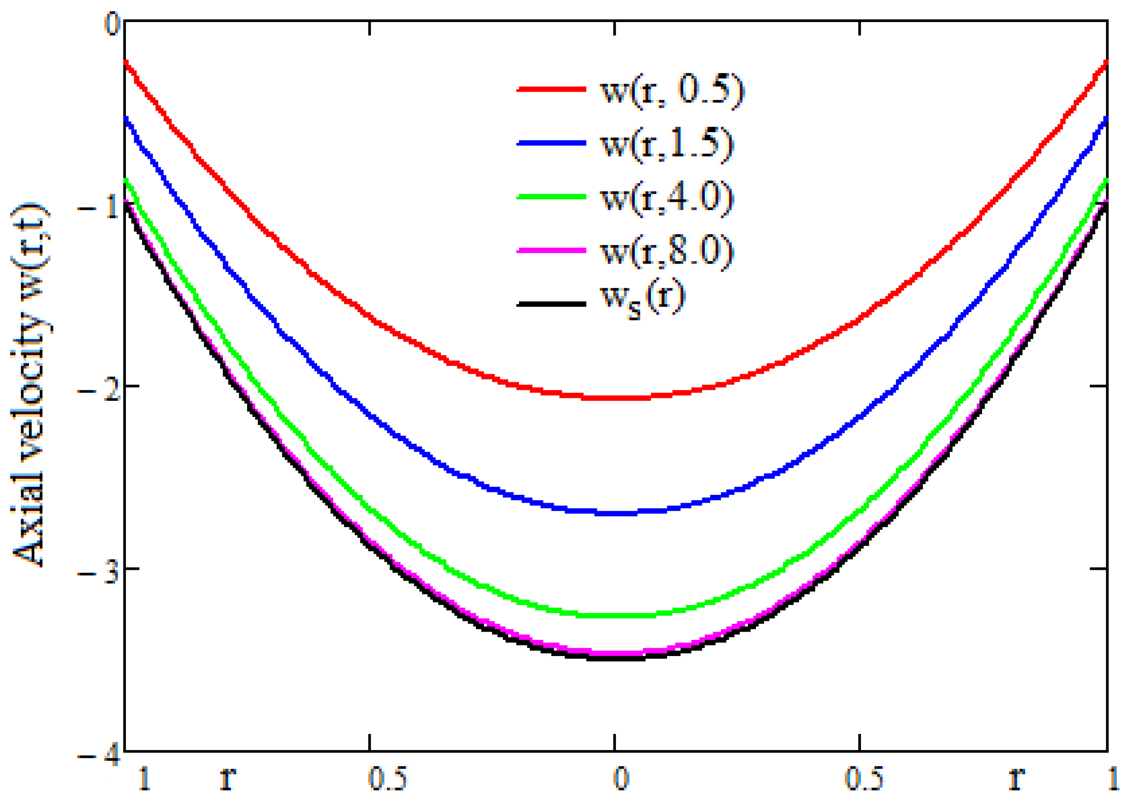
Example. This example aims to exemplify graphically that the transient solution tends to the steady-state solution for large values of time t, namely $\underset{t\to \infty }{\lim }w(r,t)=w_s(r).$ Consider the function $f(t)=1-\exp (-0.5t)$. Figure 2 shows plotted profiles of the steady-state solution $w_s(r)$ and of the transient velocity $w(r,t)$ for $t\in \{0.5, 1.5, 4.0, 8.0\}$. It is easy to see from Figure 2 that graphs of the transient velocity tend to overlap the graph of the stationary velocity when the values of time t increase.

4. Numerical Results and Discussion

Unsteady, axisymmetric granular flows based on the particle–particle model developed by Blackmore et al. [12] in the Hertz–Mindlin theory have been analytically studied. By and large, in granular flows, the density field and the pressure are unknown scalar functions. A well-known relationship between these fields gives the pressure field a power law of the density. The unsteady, axisymmetric, fully developed granular flow under the gravity action in a vertical cylindrical pipe under the assumption that the density field is constant and the velocity on the pipe’s wall is time-dependent has been investigated. Using integral transforms method and appropriate initial-boundary conditions, the analytical solution for axial velocity is determined. The obtained analytical solution is used to determine the steady-state solution (the solution for large values of the time). The properties of the flow in some particular cases of the velocity on the pipe’s surface are analyzed and the transient flow is compared with the stationary one.

The studied problem has been solved for arbitrary time-dependent values of the axial velocity on the pipe’s surface; therefore, the obtained solutions are suitable to describe several practical issues by changing the function $f(t)$ that gives the velocity on the boundary.

The analytical solution for axial velocity has been determined by two ways using Laplace transform coupled with the residue theory in complex analysis, respectively, the finite Hankel transform. The general analytical solution of the axial velocity is used to determine the steady-state solution (the solution for large values of the time). Note that the stationary solution obtained by us is identical to the one determined in ([12], Equation (31)) for the same type of movement but with constant speed on the pipeline’s surface.

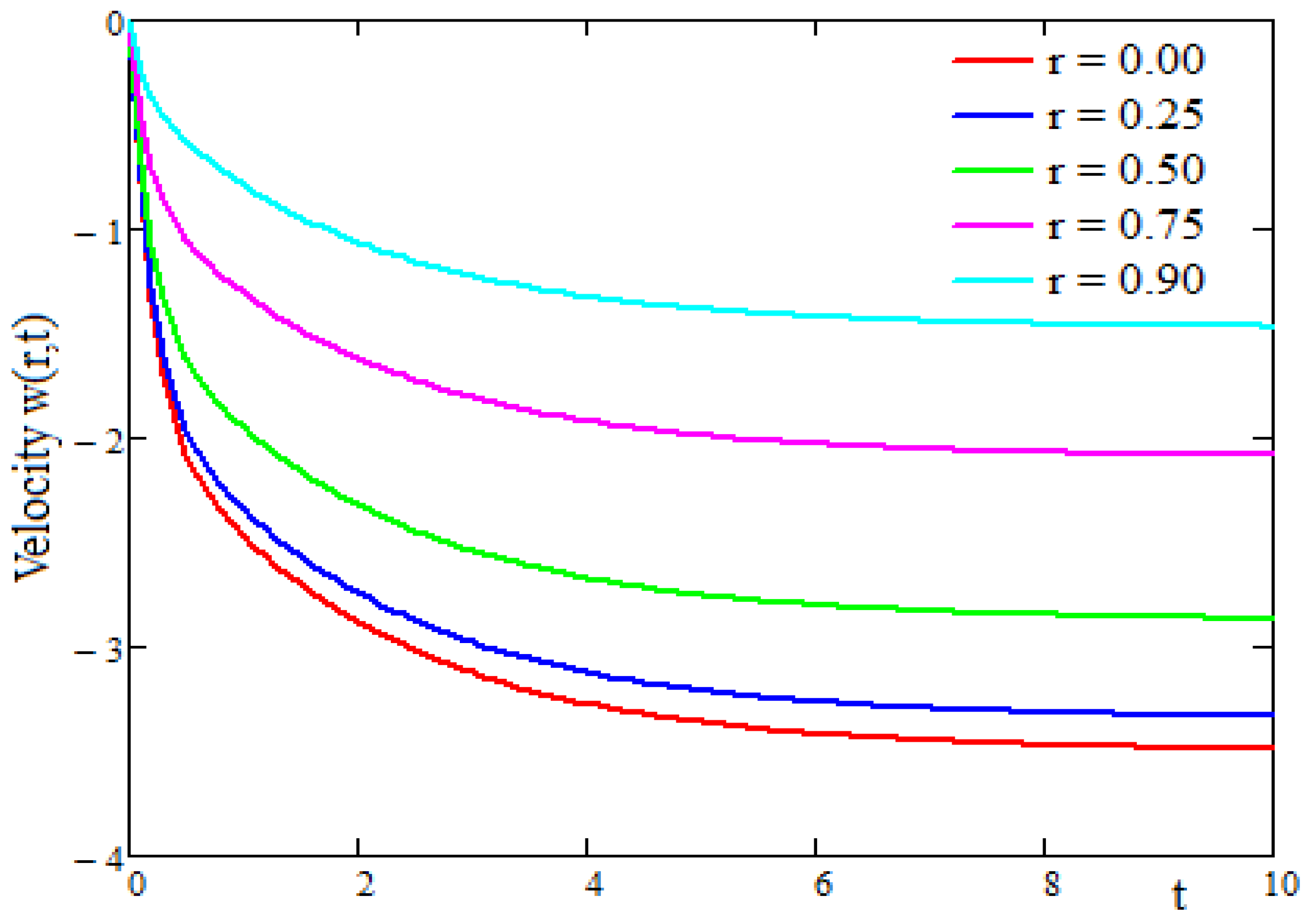
In this section, some flow characteristics are highlighted by numerical simulations and graphical illustrations obtained with the Mathcad software. To do this, we used for the boundary dimensionless axial velocity the expression $f(t)=1-\exp (-0.5t)$.

The time-variation of the dimensionless axial velocity $w(r,t)$ is given in Figure 3. The curves in Figure 3 are plotted for $a_0=10$ and five spatial positions, namely $r\in \{0, 0.25, 0.50, 0.75, 0.90\}$.

It can be seen in Figure 3 that the velocity has the highest absolute value in the central area of the pipe. Also, as expected, the transient velocity $w(r,t)$ tends to be the steady-state velocity $w_s(r)$ for large values of time t.

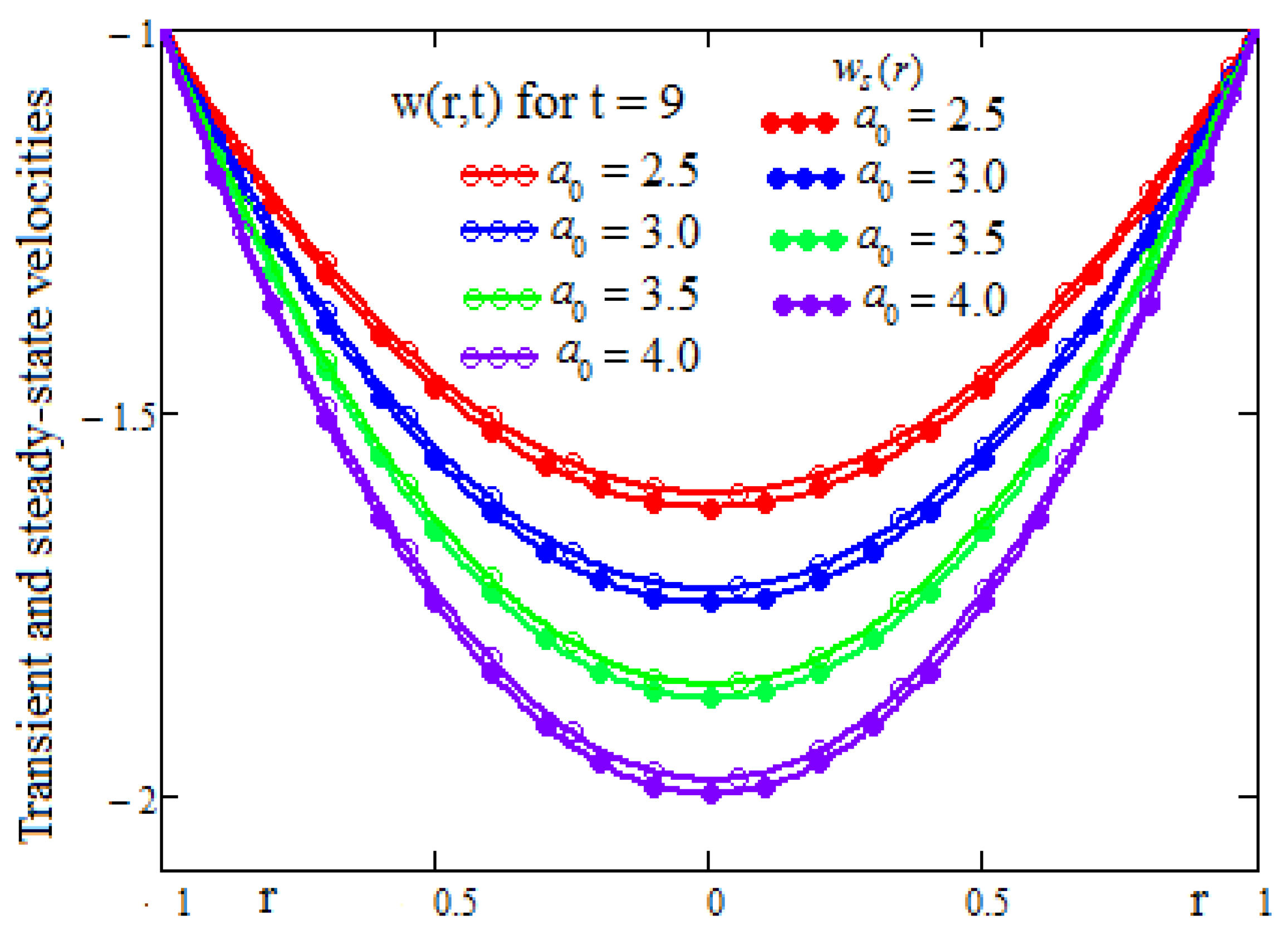
The graphs in Figure 4 were drawn to investigate the influence of the dimensionless parameter $a_0$ on the axial velocity. The axial velocity profiles in Figure 4 show that its absolute value increases with the $a_0$ parameter. This is since the viscosity of the material decreases with the increase in the values of the coefficient $a_0$. The same characteristic of the axial velocity is observed in Figure 5. The curves in this figure compare the transient velocity and the steady-state velocity for different values of the parameter $a_0$, at the moment, $t=9$.

5. Conclusions

Unsteady, axisymmetric granular flows based on the particle–particle model developed by Blackmore et al. [12] in the Hertz–Mindlin theory have been analytically studied in a particular case of the nonlinear mathematical model.

By and large, in granular flows, the density field and the pressure are unknown scalar functions. A well-known relationship between these fields gives the pressure field a power law of the density. The fully developed granular flows under gravity action in a vertical cylindrical pipe under the assumption that the density field is constant and the velocity on the pipe’s wall is time-dependent have been analytically studied.

Using integral transforms method, the analytical solution for axial velocity was determined in two different ways, namely by using Laplace transform coupled with the residues theory in complex functions, respectively, the finite Hankel transform and Bessel functions. For large values of the time t, the general solution of the axial velocity tends to be the steady-state solution known in the literature.

Flow characteristics were investigated by numerical simulations and graphical illustrations. The properties of the flow in some particular cases of the velocity on the pipe’s surface were analyzed and the transient flow was compared with the stationary one.

References

- Nedderman, R.M. Statics and Kinematics of Granular Materials; Cambridge University Press: Cambridge, UK, 1992. [Google Scholar]
- Savage, S.B.; Hutter, K. The dynamics of avalanches of granular materials from initiation to runout. Part I Analysis. Acta Mech. 1991, 86, 201–223. [Google Scholar] [CrossRef]
- Cleary, P.W.; Prakash, M. Discrete–element modelling and smoothed particle hydrodynamics: Potential in the environmental sciences. Philosophical Transactions of the Royal Society of London. Ser. A Math. Phys. Eng. Sci. 2004, 362, 2003–2030. [Google Scholar] [CrossRef] [PubMed]
- Forterre, Y.; Pouliquen, O. Flows of dense granular media. Annu. Rev. Fluid Mech. 2008, 40, 1–24. [Google Scholar] [CrossRef]
- Williams, H. Gravity-driven granular flows in pipes: Teaching experimental skills in the context of granular flows. Phys. Educ. 2022, 57, 055024. [Google Scholar] [CrossRef]
- Barker, T.; Zhu, C.; Sun, J. Exact solutions for steady granular flow in vertical chutes and pipes. J. Fluid Mech. 2022, 930, A21. [Google Scholar] [CrossRef]
- Farin, M.; Mangeney, A.; De Rosny, J.; Toussaint, R.; Trinh, P.T. Link between the dynamics of granular flows and the generated seismic signal: Insights from laboratory experiments. J. Geophys. Res. Earth Surf. 2018, 123, 1407–1429. [Google Scholar] [CrossRef]
- Ligneau, C.; Sovilla, B.; Gaume, J. Numerical investigation of the effect of cohesion and ground friction on snow avalanches flow regimes. PLoS ONE 2022, 17, e0264033. [Google Scholar] [CrossRef] [PubMed]
- Yang, S.; Wang, X.; Liu, Q.; Pan, M. Numerical simulation of fast granular flow facing obstacles on steep terrains. J. Fluids Struct. 2020, 99, 103162. [Google Scholar] [CrossRef]
- Fazelpour, F.; Daniels, K.E. The effect of boundary roughness on dense granular flows. EDP Sciences. EPJ Web Conf. 2021, 249, 03014. [Google Scholar] [CrossRef]
- Zhu, H.P.; Yu, A.B. Steady-state granular flow in a 3D cylindrical hopper with flat bottom: Macroscopic analysis. Granul. Matter 2005, 7, 97–107. [Google Scholar] [CrossRef]
- Blackmore, D.; Samulyak, R.; Rosato, A. New Mathematical Models for Particle Flow Dynamics. J. Nonlinear Math. Phys. 1999, 6, 198–221. [Google Scholar] [CrossRef][Green Version]
- Legree, P.Y.; Staron, L.; Popinet, S. Granular column collapse as a continuum: Validity of a two-dimensional Navier_Stokes model with a rheology. J. Fluid Mech. 2011, 686, 378–408. [Google Scholar] [CrossRef]
- Shabir, A.; Siraj, M.S. DEM study of monodisperse granular flow in a pipe. Adv. Powder Thech. 2020, 31, 4222–4230. [Google Scholar] [CrossRef]
- Li, T.; Zhang, H.; Liu, M.; Huang, Z.; Bo, H.; Do, Y. DEM study of granular discharge rate through a vertical pipe with a bend outlet in small absorber system. Nucl. Eng. Des. 2017, 314, 1–10. [Google Scholar] [CrossRef]
- Rosato, A.D.; Zuo, L.; Blackmore, D.; Wu, H.; Horntrop, D.J.; Parker, D.J.; Windows-Yule, C. Tapped granular column dynamics: Simulations, experiments and modeling. Comput. Part. Mech. 2016, 3, 333–348. [Google Scholar] [CrossRef]
- Barker, T.; Rauter, M.; Maguire, E.S.F.; Johnson, C.G.; Gray, J.M.N.T. Coupling rheology and segregation in granular flows. J. Fluid Mech. 2021, 909, A22. [Google Scholar] [CrossRef]
- Heyman, J.; Delannay, R.; Tabuteau, H.; Valance, A. Compressibility regularizes the μ(I)-rheology for dense granular flows. J. Fluid Mech. 2017, 830, 553–568. [Google Scholar] [CrossRef]
- Kim, S.; Kamrin, K. Power-law scaling in granular rheology across flow geometries. Phys. Rev. Lett. 2020, 125, 088002. [Google Scholar] [CrossRef]
- Elata, D.; Berryman, J.G. Contact force displacement laws and the mechanical behavior of random packs of identical spheres. Mech. Mater. 1996, 24, 229–240. [Google Scholar] [CrossRef]
- Jiang, M.; Shen, Z.; Wang, J. A novel three-dimensional contact model for granulates incorporating rolling and twisting resistances. Comput. Geotech. 2015, 65, 147–163. [Google Scholar] [CrossRef]
- Davies, B. Integral Transforms and Their Applications; Springer Science & Business Media: Berlin, Germany, 2002. [Google Scholar]
- Debnath, L.; Bhatta, D. Integral Transforms and Their Applications; Chapman and Hall/CRC: London, UK, 2016. [Google Scholar]
- Watson, G.N. A Treatise on the Theory of Bessel Functions; Cambridge University Press: Cambridge, UK, 1922. [Google Scholar]
- Grigoletto, E.C.; de Oliveira, E.C. A Note on the Inverse Laplace Transform. Cad. IME-Série Matemática 2018, 39–46. [Google Scholar] [CrossRef]
- Kerimov, M.K. Studies on the zeros of Bessel functions and methods for their computation. Comput. Math. Math. Phys. 2014, 54, 1337–1388. [Google Scholar] [CrossRef]
- Roberts, G.E.; Kaufman, H. Table of Laplace Transforms; W.B. Saunders Co.: Toronto, ON, Canada, 1966. [Google Scholar]