Stochastic Intermittency Fields in a von Kármán Experiment

Abstract

We discuss the application of stochastic intermittency fields to describe and analyse the statistical properties of time series of the generalised turbulence intensity in an anisotropic and inhomogeneous turbulent flow and provide a parsimonious description of the one-, two-, and three-point statistics. In particular, we show that the three-point correlations can be predicted from observed two-point statistics. Our analysis is motivated by observed stylised features of the energy dissipation in homogeneous and isotropic situations where these statistical properties are well represented within the framework of stochastic intermittency fields. We find a close resemblance and conclude that stochastic intermittency fields may be relevant in more general situations.

1. Introduction

Cascade processes and their representation in terms of stochastic intermittency fields constitute a fundamental stochastic framework that captures strongly intermittent fluctuations and long range correlations with scaling properties [1,2,3,4,5,6,7]. These cascade processes have therefore found widespread applications in the phenomenological description and modelling of temporal dynamics and spatial structures in turbulent flows [8,9,10,11,12,13].

From an experimental point of view, spatial structures are often analysed in the time domain, using the Taylor Frozen Flow Hypothesis (TFFH) [14]. TFFH requires that the mean flow transports spatial structures without relevant distortion over the observation point where time series are recorded. In such situations, statistical properties associated with spatial structures are observed in the time domain and afterwards translated to and interpreted in the spatial domain [8,15,16,17,18,19,20]. However, timewise experimental studies of spatio-temporal phenomena may reveal stylised statistical features that can be used as robust characteristics of the underlying dynamics in cases where the interpretation in the spatial domain using TFFH is questionable or impossible.

In this paper, we analyse the generalised turbulence intensity in a von Kármán Experiment with focus on a particular set of such statistical properties and their realisation within the framework of stochastic intermittency fields, namely self-scaling of correlators [9] and the representation of three-point statistics in terms of two-point statistics [2,10]. These temporal statistical properties are well represented within stochastic intermittency fields and their empirical verification has been done for the statistics of the energy dissipation in isotropic and homogeneous turbulent flows [9,10,13]. One of our main results is that the statistical properties displayed by correlators in homogeneous and isotropic flows are also observed in non-homogeneous and non-isotropic situations where an interpretation in terms of spatial structures is not possible. Thus, our analysis shows that these specific statistical properties of correlators are not necessarily related to spatial dynamics and as such are genuine time wise properties. Based on that, we propose that stochastic intermittency fields and the statistical properties implied by them may be of relevance in a wider range of applications than previously anticipated.

The paper is organised as follows. In Section 2, we give some background on the data we analysed and briefly outline the analysis of the generalised turbulence intensity as reported in [21]. Section 3 introduces stochastic intermittency fields together with some of their most important statistical properties. We examine these statistical properties for the generalised turbulence intensity in Section 4. Section 5 concludes and summarises the main results.

2. The Generalised Turbulence Intensity

Our data set is recorded within the von Kármán Experiment (VKE), performed at the Commissariat á l’Énergie Atomique in Paris. The experiment consists of a realisation of the von Kármán swirling flow, inertially-driven between two disks fitted with blades, and with Reynolds number $Re={10}^5$, described in detail in [22].

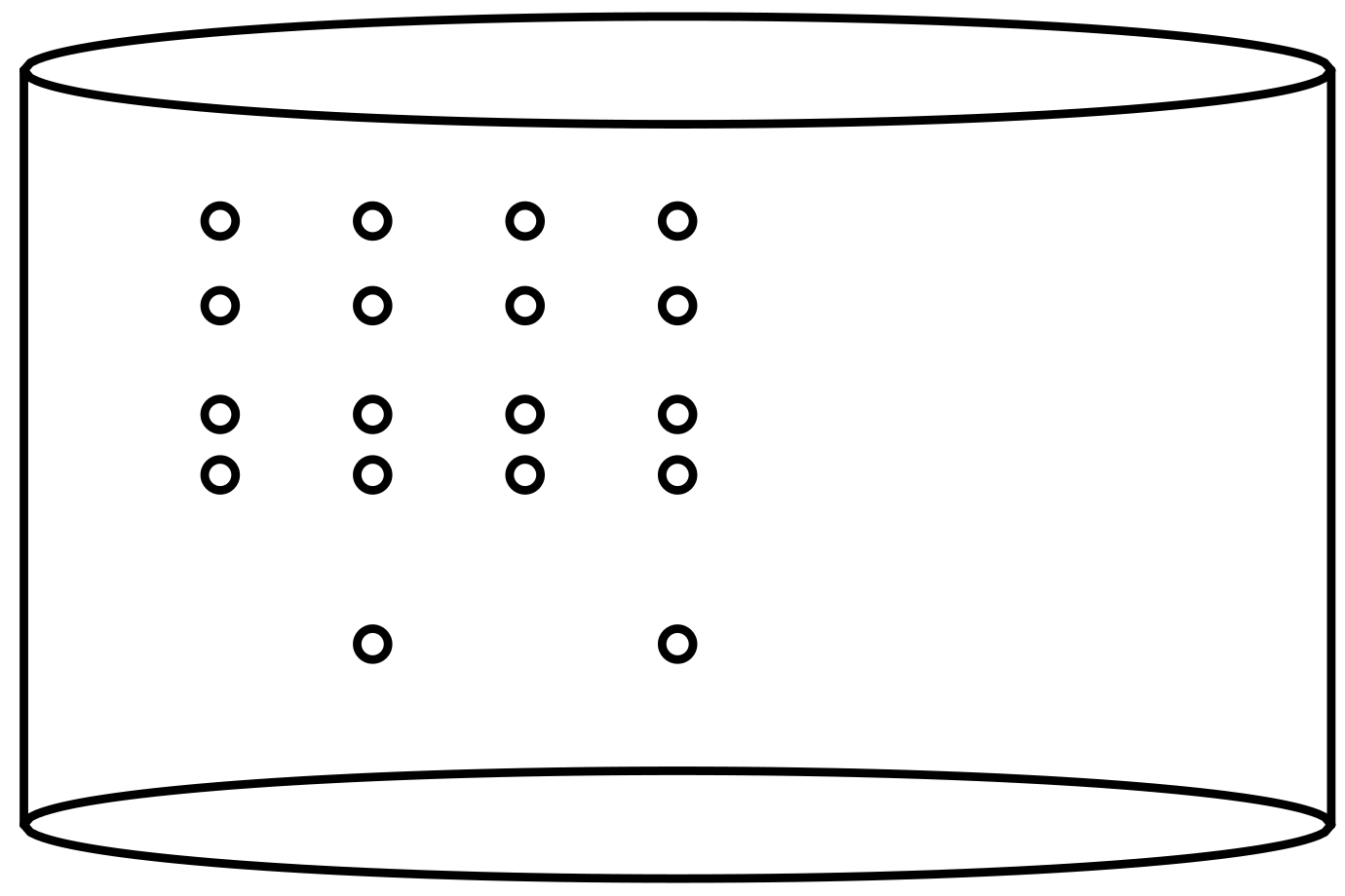
The fluid is seeded with passive particles that sample the fluid velocity field on a $11\times 17$ spatial point grid by means of Laser Doppler Velocimetry (LDV). The measurements provide the azimuthal component of the velocity vector with an average data rate of ∼0.5 kHz. Following the recommendation in [23], time series affected by spurious data and boundary effects are discarded in the present analysis implying that, out of the original 187 time series, only 18 are retained. In [23], the authors state that, for these 18 time series, they are confident that the LDV is capable of measuring the vertical velocity component. The location of the 18 measurement points within the experimental device is sketched in Figure 1.

The velocities of the tracer particles are measured over a fixed period $T_0=3600$ s. The sample size at each location depends on the number of tracer particles passing by, implying that the length of the measured time series is ranging from n = 1,435,270 to n = 2,462,311. Moreover, the measurements are not equidistant.

In [21], different realisations of the VKE, sampled by Stereoscopic Particle Image Velocimetry, are considered, producing equidistant time series of velocities on a $58\times 58$ point grid. The data rate is lower and the time series are shorter compared to the LDV case. The authors then introduce a so-called generalised turbulence intensity

$$\tilde{\delta }\left(t\right)=\frac{\langle v^2\left(t\right)\rangle }{\langle {\overline{v}}^2\rangle }$$

(1)

where $\langle ·\rangle$ denotes spatial averaging and $\overline{·}$ denotes time wise averaging. Here, and in what follows, spatial averaging refers to an ensemble average of the time series after regularisation in time [23]. This quantity measures the contribution of the instantaneous kinetic energy of the field to the kinetic energy of the mean field. The spatial averaging in (1) turns it into a global observable for the VKE.

It is argued in [21] that the generalised turbulence intensity (1) serves as a quantitative measure for the level of fluctuations compared to the mean flow and their ability to disturb the mean flow. This characterisation relies on two parameters, the mean value and variance of $\tilde{\delta }$. It is important to note that one of the main arguments behind this point of view is the assumption of a Gaussian probability density function (pdf) for $\tilde{\delta }$. Moreover, the analysis in [21] solely focuses on marginal statistical properties, not taking into account the dynamics of $\tilde{\delta }$. In Section 4, we will show that the Gaussian assumption may well be questioned for our data set and that the dynamical behaviour of a slightly modified version of the generalised turbulence intensity reveals distinct statistical properties that may serve to better characterise the various realisations of the VKE experiments.

The analysis performed in Section 4 requires evenly spaced time series. To overcome the problem of irregular sampling in time in our data set, we define a suitable regular partition of the total time interval $[0,T_0]$ in each of our time series and, as a consequence, slightly modify definition (1). We choose a constant time interval $\Delta t$ as the global average waiting time for five measurements in the whole data set. We verified that, in this way, we avoid considering time intervals without any measurement, with no drastic decrease in the length of the resulting time series and of the corresponding sampling frequency. A reasonable value is $\Delta t=9.27$ ms. We then define evenly spaced time points $t_m=m·\Delta t$, $m=0,1,\dots ,M$, $M=⌊\frac{T_0}{\Delta t}⌋$ = 388,267.

Considering this partition, we replace the instantaneous value of the velocity component $v\left(t\right)$ in (1) by the mean velocity within each time step

$$v\left(t_m\right)=\frac{1}{n}\sum _{h=1}^n{v}_h,$$

where n is the number of measurements $v_h$ in $]t_{m-1},t_m]$. The modified expression for the generalised turbulence intensity then reads

$$\delta \left(t_m\right)=\frac{\langle v^2\left(t_m\right)\rangle }{\langle {\overline{v}}^2\rangle }.$$

(2)

3. Stochastic Intermittency Fields

Stochastic intermittency fields have been introduced as a suitable stochastic framework that accounts for the specific scaling behaviour of correlators of the turbulent energy dissipation [1]. These fields predicted statistical properties that go beyond the original motivation by scaling of correlators and were subsequently verified empirically [9,10]. Relevant for the present analysis of the generalised turbulence intensity $\delta$ (2) with respect to stochastic intermittency fields are self-scaling of correlators (9) and a specific relation between three-point correlators and two-point correlators (11).

3.1. Lévy Based Model Construction

The basic ingredient for the construction of stochastic intermittency fields is that of an infinitely divisible and independently scattered random measure, called a Lévy basis. Such measures associate an infinitely divisible random variable to any bounded subset of the underlying space S. For disjoint subsets, the associated variables are independent, and the random variable associated with a disjoint union of sets almost surely equals the sum of the random variables associated with each of the individual sets (see [24,25] and references therein for more detail and mathematical rigour).

Here, we restrict to the case of a homogeneous Lévy basis, where the distribution of the measure does not depend on the localisation of the subset and where the control measure is proportional to the Lebesgue measure. In this case, it is straightforward to define integrals with respect to the Lévy basis.

Let Z be a homogeneous Lévy basis on $S\subset {\mathbb{R}}^n$. Then, for $x\in S$, we choose $S^{\prime }\left(x\right)\subset S$, $x\in S^{\prime }\left(x\right)$, and define a stochastic intermittency field as

$$y\left(x\right)=exp\left\{{\int }_{S^{\prime }\left(x\right)}h\left(a\right)Z\left(\mathrm{d}a\right)\right\},$$

where h is a deterministic kernel (subject to some minor conditions to ensure the existence of the above integral).

We have the fundamental relation

$$\mathrm{E}\left\{exp\left[{\int }_{S^{\prime }}h\left(a\right)Z\left(\mathrm{d}a\right)\right]\right\}=exp\left\{{\int }_{S^{\prime }}\mathrm{K}\left[h\left(a\right)\right]\mathrm{d}a\right\},$$

(3)

where $\mathrm{E}$ denotes the expectation and $\mathrm{K}[·]\mathrm{d}a$ denotes the cumulant function of $Z\left(\mathrm{d}a\right)$, defined by

$$ln\mathrm{E}\left\{exp\left(\xi Z\right(\mathrm{d}a\left)\right)\right\}=\mathrm{K}\left[\xi \right]\mathrm{d}a.$$

(4)

Relation (3) allows for explicitly calculating and modelling the correlation structure of the stochastic intermittency field y.

A particular simple example of a stochastic intermittency field is

$$\epsilon \left(x\right)=exp\left\{{\int }_{S^{\prime }\left(x\right)}Z\left(\mathrm{d}a\right)\right\},$$

(5)

where $S^{\prime }\left(x\right)=x+S_0$ for some fixed $S_0\subset S$, $x\in S$. The set $S^{\prime }$ is termed ambit set in [26] (a comprehensive account of so-called ambit stochastics may be found in [25]). Since the shape and size of the ambit set $S^{\prime }$ does not depend on the location x, the resulting process $\epsilon$ is homogeneous.

The simplified model (5) has been used in [9,10,13] to model cascade processes that capture the statistics of the energy dissipation in homogeneous, isotropic, and stationary turbulent flows. For that, the shape of $S_0$ has been chosen such that correlators and moments of the coarse grained field display scaling relations. Such scaling relations are considered as defining properties of an underlying cascade process [8].

3.2. The Self-Scaling Property

Depending on the shape and size of the ambit set $S_0$, a wide range of correlations can be modelled. In what follows, we focus on statistical properties that are independent of the shape and size of the ambit set and are solely due to the multiplicative structure of stochastic intermittency fields of type (5).

The multiplicative structure inherent to (5) can be characterised using k-point correlators of order $\overrightarrow{n}=(n_1,\dots ,n_k)$ defined as

$$c_{\overrightarrow{n}}(x_1,\dots ,x_k)=\frac{\mathrm{E}\left\{\epsilon {\left(x_1\right)}^{n_1}\cdots \epsilon {\left(x_k\right)}^{n_k}\right\}}{\mathrm{E}\left\{\epsilon {\left(x_1\right)}^{n_1}\right\}\cdots \mathrm{E}\left\{\epsilon {\left(x_k\right)}^{n_k}\right\}}.$$

(6)

These correlators can all be expressed in terms of the Euclidean volume of overlaps $V(S^{\prime }\left(x_i\right)\cap S^{\prime }\left(x_j\right))$, $i,j=1,\dots ,k$ and the corresponding constants

$$\overline{\mathrm{K}}[n_i,n_j]=\mathrm{K}[n_i+n_j]-\mathrm{K}\left[n_i\right]-\mathrm{K}\left[n_j\right].$$

(7)

For $k=2$ and $\overrightarrow{n}=(n_1,n_2),$ one obtains

$$c_{\overrightarrow{n}}(x_1,x_2)=exp\left\{\overline{\mathrm{K}}[n_1,n_2]V(S^{\prime }\left(x_1\right)\cap S^{\prime }\left(x_2\right))\right\}.$$

(8)

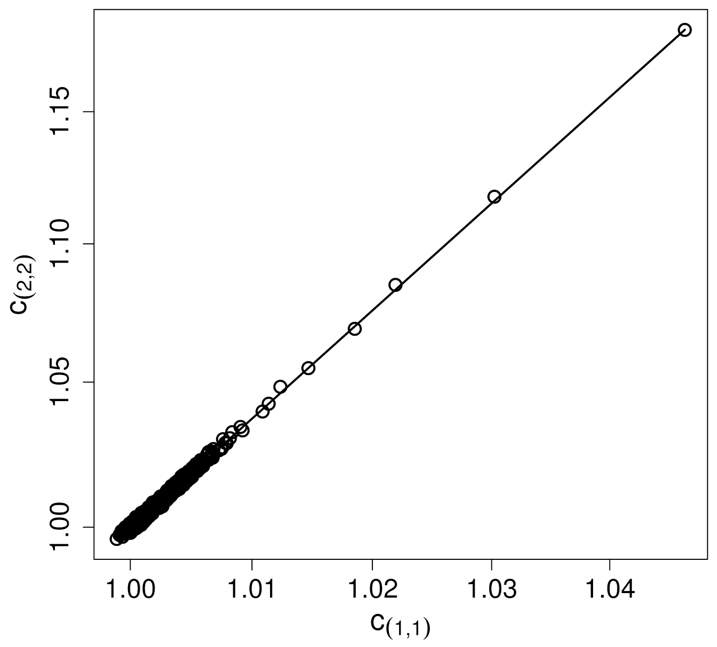
Here, the properties of the underlying Lévy basis are separated from the properties of the associated sets $S^{\prime }$, which allows for representing correlators of order $\overrightarrow{m}=(m_1,m_2)$ as a scaling relation of correlators of order $\overrightarrow{n}=(n_1,n_2)$ [9]

$$c_{\overrightarrow{m}}(x_1,x_2)=c_{\overrightarrow{n}}{(x_1,x_2)}^{r(\overrightarrow{m},\overrightarrow{n})}$$

(9)

where

$$r(\overrightarrow{m},\overrightarrow{n})=\frac{\overline{\mathrm{K}}[m_1,m_2]}{\overline{\mathrm{K}}[n_1,n_2]}.$$

(10)

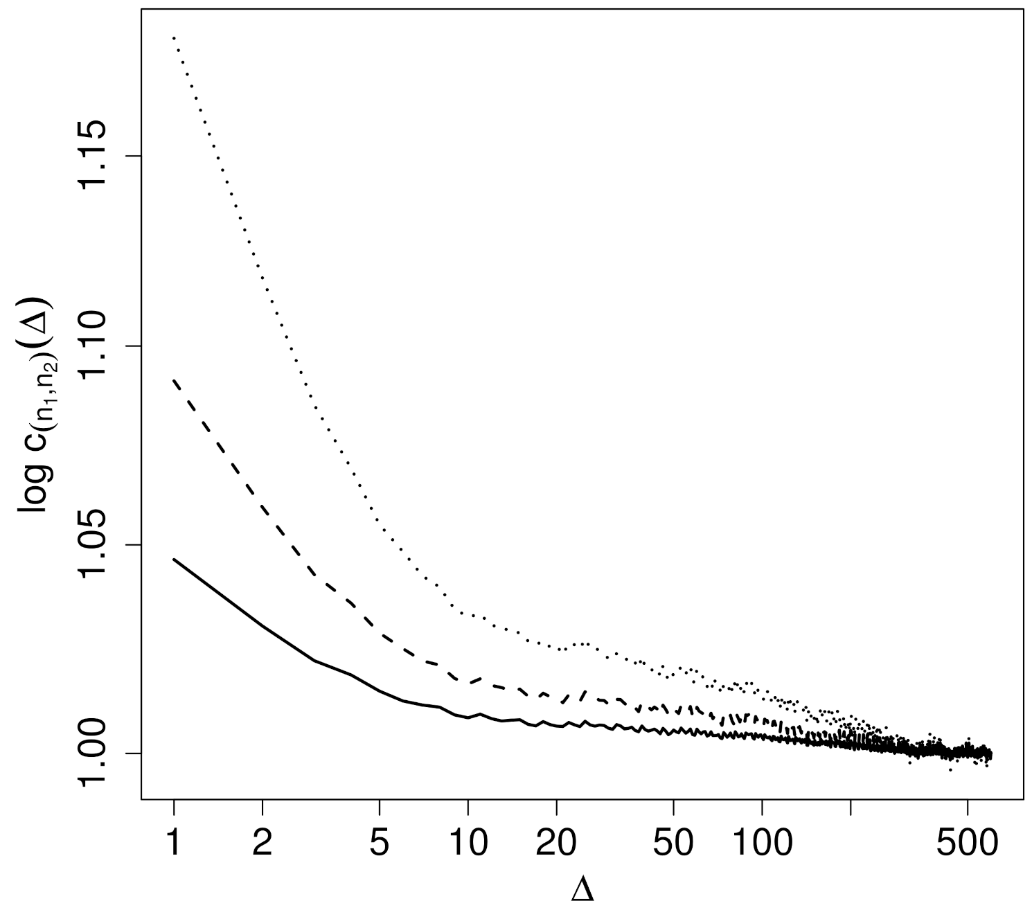
This self-scaling property is independent of the shape and size of the associated ambit sets $S^{\prime }$ (and thus independent of the specific behaviour of the correlators) and only depends on the properties of the underlying Lévy basis.

It is important to note that processes revealing scaling relations for two-point correlators trivially exhibit self-scaling of correlators. For the energy dissipation in homogeneous and isotropic flow situations, the important observation is that the range where self-scaling is observed considerably extends the range where scaling of correlators is detected [9].

3.3. Three-Point Correlators

The second fingerprint of an underlying stochastic intermittency field of the type (5) that is independent of the shape and size of the ambit set concerns the behaviour of three-point correlators in terms of two-point correlators. We illustrate the relation between three-point correlators and two-point correlators in a simplified setting. For simplicity, we set $\mathrm{E}\left\{\epsilon \left(x\right)\right\}=1$, i.e., $\mathrm{K}\left[1\right]=0$, without loss of generality. 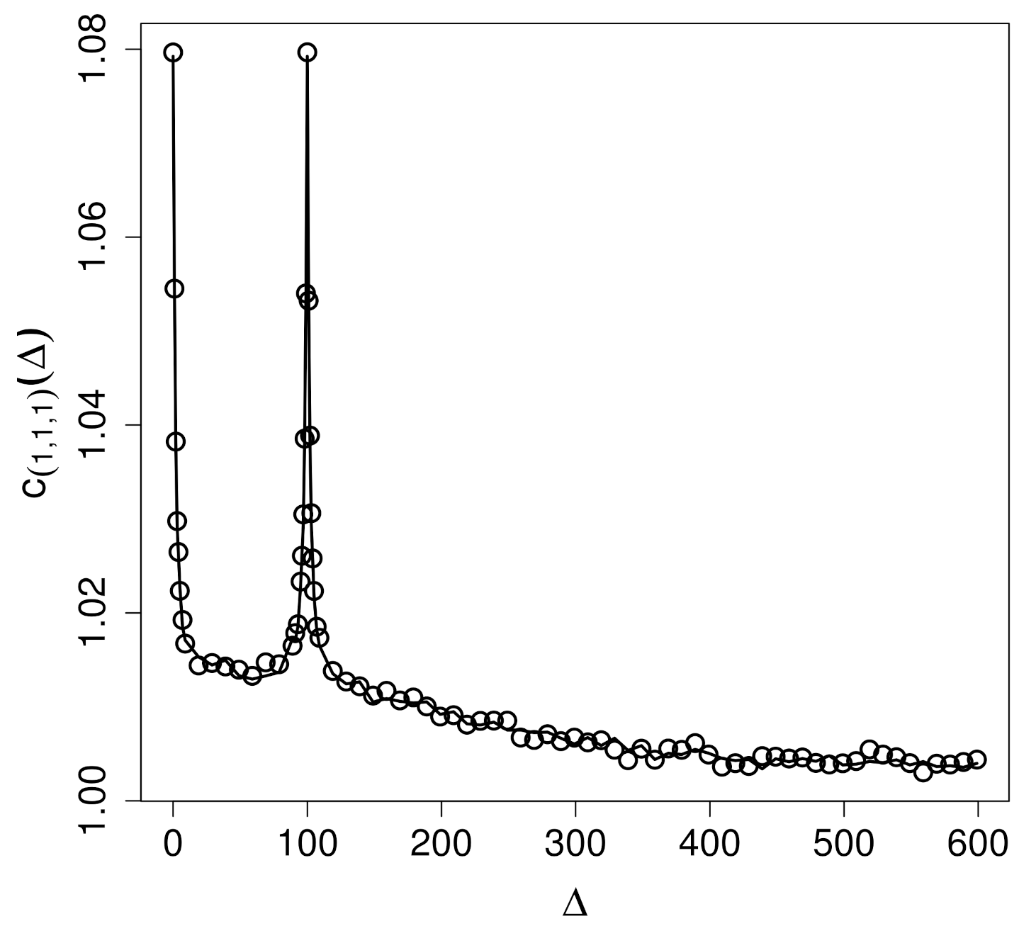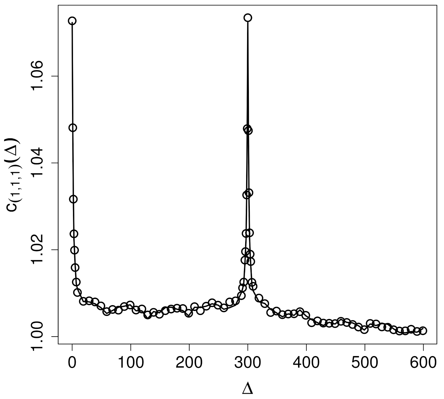We also specify the underlying space to be $S=\mathbb{R}$ (for the sake of simplicity) and the associated ambit sets as $S^{\prime }\left(x\right)=[x-L,x]$, where $L>0$ denotes a decorrelation distance. The three-point correlators of order $\overrightarrow{n}=(1,1,1)$ for $x_1\le x_2\le x_3$ can then be expressed in terms of two-point correlators as (see [2,10] for details of the derivation in a more general setting)

$$\begin{array}{cc}\hfill c_{\overrightarrow{n}}(x_1,x_2,x_3)=& exp\left\{\mathrm{K}\left[2\right]V((S^{\prime }\left(x_1\right)\cap S^{\prime }\left(x_2\right))\backslash S^{\prime }\left(x_3\right))\right\}\hfill \\ \hfill & exp\left\{\mathrm{K}\left[2\right]V((S^{\prime }\left(x_2\right)\cap S^{\prime }\left(x_3\right))\backslash S^{\prime }\left(x_1\right))\right\}\hfill \\ \hfill & exp\left\{\mathrm{K}\left[3\right]V(S^{\prime }\left(x_1\right)\cap S^{\prime }\left(x_3\right))\right\}\hfill \\ \hfill =& \frac{c_{(1,1)}(x_1,x_2)}{c_{(1,1)}(x_1,x_3)}\frac{c_{(1,1)}(x_2,x_3)}{c_{(1,1)}(x_1,x_3)}{c}_{(2,1)}(x_1,x_3)c_{(1,1)}(x_1,x_3)\hfill \\ \hfill =& c_{(1,1)}(x_1,x_2)c_{(1,1)}(x_2,x_3)c_{(1,1)}{(x_1,x_3)}^{r\left(\right(2,1),(1,1\left)\right)-1}.\hfill \end{array}$$

(11)

Three-point correlators of order $(1,1,1)$ are completely determined by the two-point correlators of order $(1,1)$ and the self-scaling exponent $r\left(\right(2,1),(1,1\left)\right)$. Equation (11) is the second implication of an underlying stochastic intermittency field of the type (5) that we will confront the generalised turbulence intensity $\delta$ with.

Formula (11) is derived here for the simple case of ambit sets in $\mathbb{R}$. However, as was shown in [2], a corresponding identical relation can also be derived for more general ambit sets in ${\mathbb{R}}^n$ as long as the positions $x_1,x_2$, and $x_3$ are along the same coordinate axis and the associated ambit sets have a finite Euclidean volume. Furthermore, it can be shown that arbitrary n point correlators can be expressed in terms of two-point correlators and a suitable set of self-scaling exponents.

4. Statistical Properties of the Generalised Turbulence Intensity

In the following sections, we analyse the generalised turbulence intensity $\delta$ with respect to two-point and three-point statistics and provide empirical evidence for the properties (9) and (11). We complement the analysis by a discussion of the marginal law of $\delta$ within the class of normal inverse Gaussian distributions and emphasise the non-Gaussian character in relation to the analysis performed in [21].

4.1. Marginal Distribution of the Generalised Turbulence Intensity

The assumption of a Gaussian distribution for the generalised turbulence intensity is the starting point for the characterisation of different experimental realisations of the VKE in [21]. Here, we analyse the log amplitude of the generalised turbulence intensity $\delta$ within the class of normal inverse Gaussian (NIG) distributions which constitute a parsimonious and flexible class of infinitely divisible distributions that include the Gaussian law as a limiting case (see Appendix A). It is natural to investigate the distribution of $log\delta$ which in the framework of stochastic intermittency fields of type (5) relates to the law of the underlying Lévy basis.

Figure 2 shows the probability density function (pdf) of $\delta$ together with the corresponding approximations obtained from a fit of the pdf of $\delta$ within the class of Gaussian distributions and a fit of the pdf of $log\delta$ within the class of NIG distributions. The estimated log-NIG distribution excellently fits the empirical density and is clearly superior to the Gaussian distribution, able to capture the asymmetry and the detailed tail behaviour. The mean squared error [27] of the Gaussian approximation is $5.3\times {10}^{-4}$, while that for the approximation within the class of NIG distributions is $2.6\times {10}^{-6}$. The maximum likelihood estimates of the parameters of the NIG distribution are $\mu =2.087$, $\delta =1.066$, $\alpha =40.269$, and $\beta =-28.708$. The four parameters for the NIG distribution reflect the four main properties of the pdf of $\delta$, the mean, the variance, and the specific tail behaviour including its asymmetry (see Appendix A for details).

It is of interest to inquire the dynamical role of the additional parameters of the NIG distribution in relation to the analysis performed in [21] based on the assumption of a Gaussian distribution for $\delta$. This is, however, outside the scope of the present analysis and postponed to a forthcoming study. Another interesting point is the fact that a similar analysis within the class of NIG distributions has been performed for the energy dissipation in various homogeneous and isotropic turbulent experiments [13] with similar excellent fits.

4.2. Two-Point Correlators of $\delta$

As a first dynamical statistical property of $\delta$, we analyse two-point correlators $c_{\overrightarrow{n}}(\Delta )$ of $\delta$, $\overrightarrow{n}=(n_1,n_2)$, where $\Delta$ denotes the time lag $\Delta =t_2-t_1\ge 0$ and where

$$c_{\overrightarrow{n}}(\Delta )=\frac{\mathrm{E}\left\{\delta {\left(t_1\right)}^{n_1}\delta {\left(t_2\right)}^{n_2}\right\}}{\mathrm{E}\left\{\delta {\left(t_1\right)}^{n_1}\right\}\mathrm{E}\left\{\delta {\left(t_2\right)}^{n_2}\right\}}$$

(12)

only depends on $\Delta$ due to stationarity of $\delta \left(t\right)$.

Figure 3 shows these correlators for $\overrightarrow{n}=(1,1),(1,2)$ and $(2,2)$. With increasing order $\overrightarrow{n}$, the scatter at large time lags increases and we therefore restrict the discussion to the relatively low orders displayed in Figure 3.

Figure 4 and Figure 5 show the functional dependence between correlators of different orders in double logarithmic representation. A self-scaling relation of the form

$$c_{\overrightarrow{m}}(\Delta )=c_{\overrightarrow{n}}{(\Delta )}^{r(\overrightarrow{m},\overrightarrow{n})}$$

(13)

will result in a straight line where the slope is given by the self-scaling exponent r. Self-scaling of correlators is well established for the generalised turbulence intensity $\delta$ and holds for all time lags $\Delta$ covered by Figure 3. The estimated self-scaling exponents are $r\left(\right(1,2),(1,1\left)\right)=1.92$ and $r\left(\right(2,2),(1,1\left)\right)=3.69$. The ratio of these exponents may be expressed as, using (7) and (10),

$$\frac{r\left(\right(2,2),(1,1\left)\right)}{r\left(\right(1,2),(1,1\left)\right)}=\frac{K\left[4\right]-2K\left[2\right]}{K\left[3\right]-K\left[2\right]-K\left[1\right]}.$$

For a Gaussian Lévy basis of an underlying stochastic intermittency field, this ratio is 2. In the present analysis, we get a ratio of $1.95$ expressing the fact that the Lévy basis is not Gaussian, but not too far away from the Gaussian case with respect to the modelling of the low order moments of the generalised turbulence intensity.

The self-scaling exponents $r\left(\right(1,2),(1,1\left)\right)$ and $r\left(\right(2,2),(1,1\left)\right)$ are estimated from the empirical correlators and the relation

$$log{c}_{\overrightarrow{m}}(\Delta )=r(\overrightarrow{m},\overrightarrow{n})log{c}_{\overrightarrow{n}}(\Delta )$$

using least-squares estimation. Another possibility is to extract these exponents directly from the correlators at $\Delta =0$ and the marginal law of the generalised turbulence intensity. For $\Delta =0$, the self-scaling relation (9) may be written as, assuming a NIG distribution for the generalised turbulence intensity and using the cumulant function (A2),

$$\begin{array}{cc}\hfill r\left(\right(1,2),(1,1\left)\right)=& \frac{log{c}_{(2,1)}\left(0\right)}{log{c}_{(1,1)}\left(0\right)}=\frac{log\mathrm{E}\left\{{\delta }^3\right\}-log\mathrm{E}\left\{{\delta }^2\right\}-log\mathrm{E}\left\{\delta \right\}}{log\mathrm{E}\left\{{\delta }^2\right\}-2log\mathrm{E}\left\{\delta \right\}}\hfill \\ \hfill =& \frac{-\sqrt{{\alpha }^2-{\beta }^2}-\sqrt{{\alpha }^2-{(\beta +3)}^2}+\sqrt{{\alpha }^2-{(\beta +2)}^2}+\sqrt{{\alpha }^2-{(\beta +1)}^2}}{-\sqrt{{\alpha }^2-{\beta }^2}-\sqrt{{\alpha }^2-{(\beta +2)}^2}+2\sqrt{{\alpha }^2-{(\beta +1)}^2}}\hfill \end{array}$$

and

$$\begin{array}{cc}\hfill r\left(\right(2,2),(1,1\left)\right)=& \frac{log{c}_{(2,2)}\left(0\right)}{log{c}_{(1,1)}\left(0\right)}=\frac{log\mathrm{E}\left\{{\delta }^4\right\}-2log\mathrm{E}\left\{{\delta }^2\right\}}{log\mathrm{E}\left\{{\delta }^2\right\}-2log\mathrm{E}\left\{\delta \right\}}\hfill \\ \hfill =& \frac{-\sqrt{{\alpha }^2-{\beta }^2}-\sqrt{{\alpha }^2-{(\beta +4)}^2}+2\sqrt{{\alpha }^2-{(\beta +2)}^2}}{-\sqrt{{\alpha }^2-{\beta }^2}-\sqrt{{\alpha }^2-{(\beta +2)}^2}+2\sqrt{{\alpha }^2-{(\beta +1)}^2}}.\hfill \end{array}$$

Inserting the estimated values $\alpha =40.269$ and $\beta =-28.708$ from the fitted NIG distribution for the generalised turbulence intensity gives the values $r\left(\right(1,2),(1,1\left)\right)=1.91$ and $r\left(\right(2,2),(1,1\left)\right)=3.66$ which are very close to those shown in Figure 4 and Figure 5, thus confirming the appropriateness of the NIG distribution as the marginal law of the generalised turbulence intensity.

Self-scaling of correlators is a characteristic feature of the dynamics of the turbulent energy dissipation in homogeneous and isotropic flows [9]. There, stochastic intermittency fields interpreted as spatial continuous cascade processes using TFFH provide a theoretical framework for this striking observation. However, in the present analysis, the flow is not homogeneous and isotropic. Due to the performed spatial averaging in the definition of $\delta$ (2), self-scaling of correlators can not be related to spatial structures and is thus established here as a genuine property of time series.

4.3. Three-Point Correlators of $\delta$

As a further indication of the relevance of stochastic intermittency fields in the present context, we examine the generalised turbulence intensity $\delta$ with respect to the predictability of three-point correlators from estimated two-point correlators as outlined in Equation (11). The self-scaling exponent $r\left(\right(2,1),(1,1\left)\right)$ entering (11) is extracted from Figure 4 by estimating the slope of $log{c}_{(2,1)}$ as a function of $log{c}_{(1,1)}$. To facilitate the representation, we choose a reference time lag T well inside the range of time lags where correlations are observed, $T\le L$ (i.e., where two-point correlators do not factorise and are not identical to one) and consider the three-point correlators as a function of the time lag $\Delta \ge 0$

$$c_{(1,1,1)}(\Delta )=\frac{\mathrm{E}\left\{\delta \left(t\right)\delta (t+T)\delta (t+\Delta )\right\}}{\mathrm{E}\left\{\delta \left(t\right)\right\}\mathrm{E}\left\{\delta (t+T)\right\}\mathrm{E}\left\{\delta (t+\Delta )\right\}}.$$

Equation (11) then translates into, using (12),

$$\begin{array}{cc}\hfill c_{(1,1,1)}(\Delta )=& c_{(1,1)}\left(\min \{\Delta ,T\}\right)c_{(1,1)}\left(\max \{T-\Delta ,\Delta -T\}\right)\hfill \\ & c_{(1,1)}{\left(\max \{\Delta ,T\}\right)}^{r\left(\right(2,1),(1,1\left)\right)-1}.\hfill \end{array}$$

(14)

Figure 6 and Figure 7 show the empirical three-point correlators for $T=100$ and $T=300$, respectively, compared to the prediction by stochastic intermittency fields as established in Equation (14). Similar results also hold for other choices of T (not shown). The peaks are located at $\Delta =T$ with values $c_{(2,1)}\left(T\right)$. The correspondence between data and theory is excellent and clearly confirms that three-point correlations of time series of $\delta$ are in accordance with those reflecting stochastic intermittency fields of type (5).

5. Discussion

Motivated by statistical properties observed for the energy dissipation in homogeneous and isotropic turbulent flows, the statistical properties of the generalised turbulence intensity in a non-homogeneous and non-isotropic flow situation are analysed in relation to characteristic statistics implied by stochastic intermittency fields. We observe a close resemblance with respect to the type of marginal distributions and the statistical properties of two-point and three-point correlators.

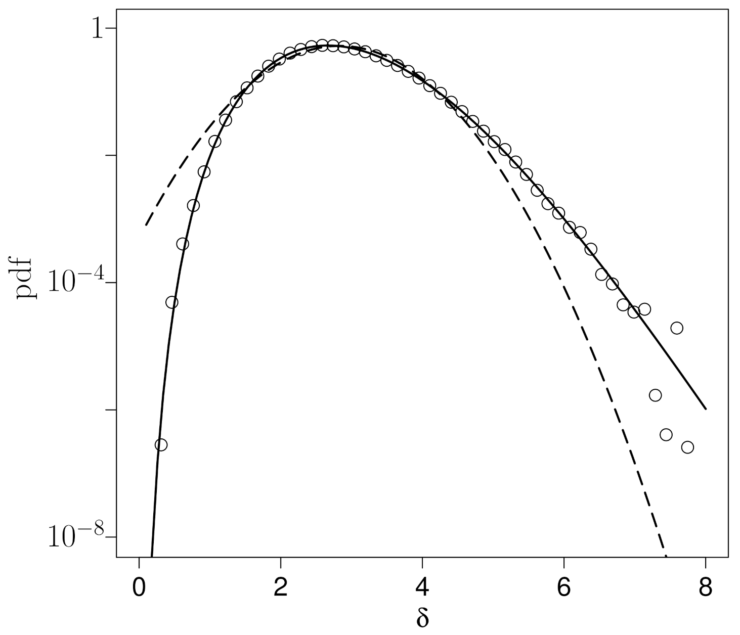
The present study reveals for the first time the appropriateness and superiority of NIG distributions compared to Gaussian distributions for the description of the marginal law of the generalised turbulence intensity. We have shown that the marginal law of the generalised turbulence intensity is parsimoniously described by a log-NIG distribution that takes into account the asymmetry and non-Gaussianity of the tails observed for the data. Compared to Gaussian approximations, this wider class of distributions is still tractable in the sense that its characteristic function is explicitly known (see Appendix A). Moreover, NIG distributions are infinitely divisible and as such may serve as the underlying Lévy basis in a stochastic intermittency framework.

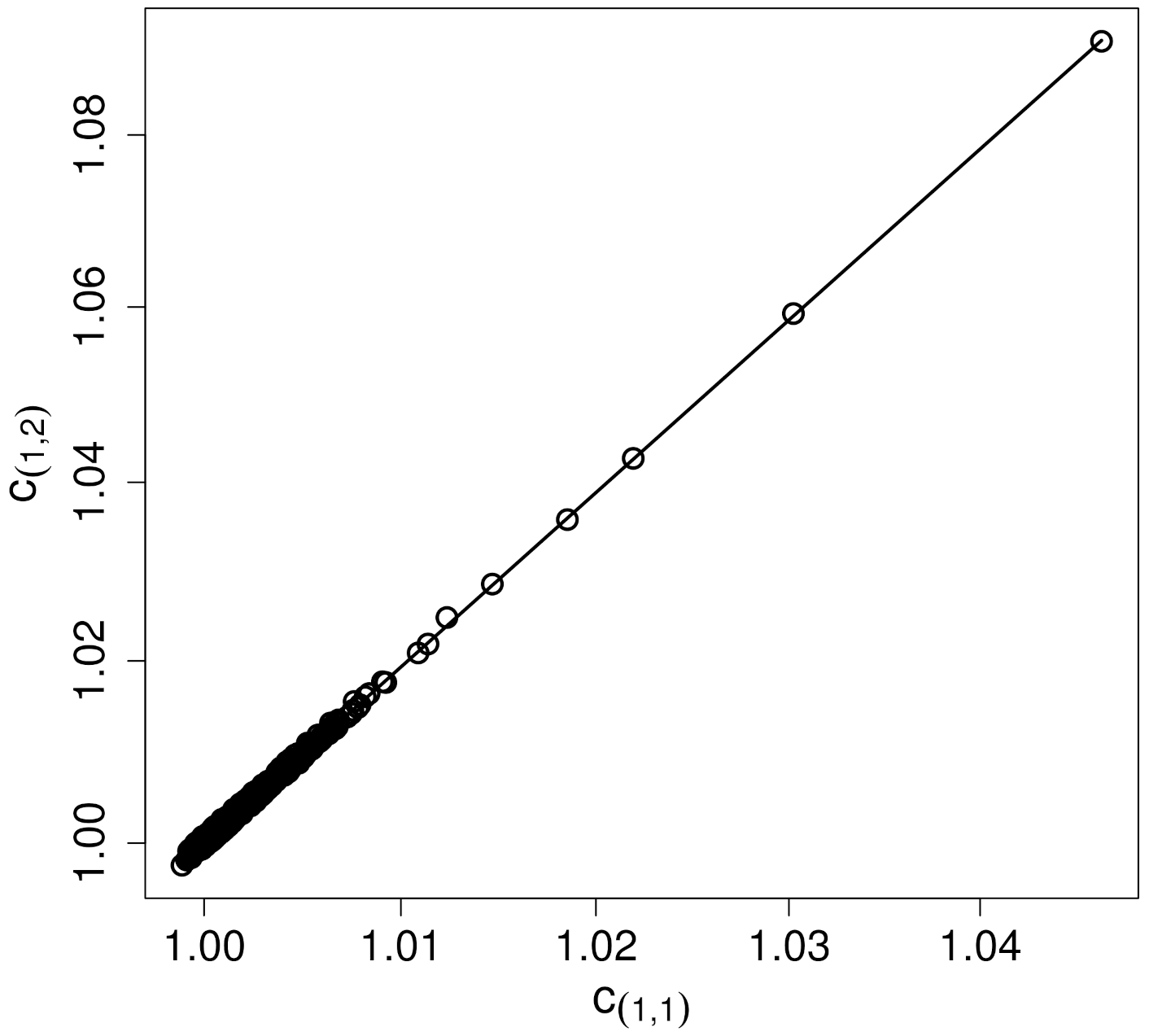
Going beyond the one-point statistics, a detailed analysis of higher order correlations of the generalised turbulence intensity provides evidence for novel stylised dynamical statistical features. In particular, we report for the first time the predictability of higher order correlations from two-point correlations. We have also shown that the generalised turbulence intensity reveals the dynamical behaviour characteristic for stochastic intermittency fields of type (5), and supplements the statistical analysis by providing a stochastic model that captures the observed statistical features. We observe self-scaling of correlators, a simple relation between two-point statistics of different orders, and a specific relation between three-point correlators and two-point correlators. In this sense, the dynamics are also described in a parsimonious way since only lowest order two-point statistics and the self-scaling exponents are needed to describe higher order two-point statistics and multi-point statistics. It remains to be examined how these additional characteristics are useful to qualitatively and quantitatively describe different flow realisations within the VKE experimental set-up in the spirit of [21].

To the best of the author’s knowledge, the proposed framework of a stochastic intermittency field of type (5) is the first explicit and analytically tractable stochastic model to describe the generalised turbulence intensity in a von Kármán Experiment. Its applicability relies on the presence of self-scaling of correlators and a specific relation between higher order correlators and two-point correlators. A full characterisation of the model requires the specification of the underlying Lévy basis and the shape and size of the associated ambit set. In the present case where the two-point correlators are monotonically decreasing, the shape and size of the ambit set can be estimated under the assumption that it is bounded by a monotonic function [9]. The underlying Lévy basis may then be estimated from the marginal distribution of the amplitude of the stochastic intermittency field using the knowledge of the shape and size of the associated ambit set [13]. A detailed analysis along these lines will be subject to a forthcoming publication.

The similarity between the statistical properties of the generalised turbulence intensity (which is based on a spatial average) to what is observed for the energy dissipation in homogeneous and isotropic situations is striking and clearly shows that these characteristic statistical properties of stochastic intermittency fields may be observed in the time domain without reference to any underlying homogeneous and isotropic spatial process. We thus conclude that the observed statistical properties of self-scaling of two-point correlators and the relation between three-point correlators and two-point correlators are of relevance in more general situations than previously reported.

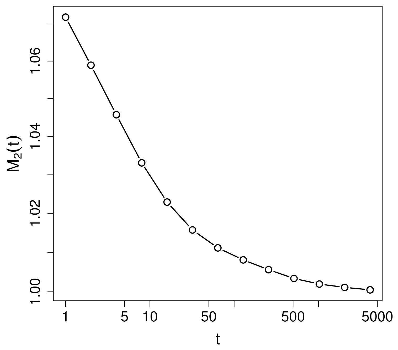
In this respect, it is also important to note that the specific dynamics of correlators are, in the present analysis, not related to a multifractal character of the analysed time series as is the case for time series of the energy dissipation in homogeneous and isotropic turbulent flows. Such a multifractality would show itself in a scaling relation for the moments of the coarse-grained intensity defined as

$$M_n\left(t\right)=\mathrm{E}\left\{{\left(\frac{1}{t}{\int }_0^t\delta \left(s\right)\mathrm{d}s\right)}^n\right\}.$$

(15)

Figure 8 displays $M_2\left(t\right)$ as a function of t in double logarithmic representation. No clear scaling behaviour can be detected. It can, however, be shown [2,9] that a pronounced scaling behaviour of $M_2$ implies scaling of $c_{(1,1)}$ from which scaling of $c_{(n_1,n_2)}$ may be expected, which, in turn, trivially implies self-scaling of correlators. Since such a sufficient scaling of $M_2$ or $c_{(n_1,n_2)}$ is not observed, self-scaling of two-point correlators may be attributed to a general class of processes that extends the class of cascade processes with multifractal scaling. Stochastic intermittency fields are a promising candidate for such a class of processes.

References

1. Barndorff-Nielsen, O.; Schmiegel, J. Lévy based tempo-spatial modelling; with applications to turbulence. Uspekhi Matematicheskikh Nauk 2003, 159, 65–90. [Google Scholar]
2. Schmiegel, J.; Barndorff-Nielsen, O.; Eggers, H. A class of spatio-temporal and causal stochastic processes, with application to multiscaling and multifractality. S. Afr. J. Sci. 2006, 101, 513–519. [Google Scholar]
3. Schmitt, F.; Marsan, D. Stochastic equations generating continuous multiplicative cascades. Eur. Phys. J. B 2001, 20, 3–6. [Google Scholar]
4. Muzy, J.; Bacry, E. Multifractal stationary random measures and multifractal random walks with log infinitely divisible scaling laws. Phys. Rev. E 2002, 66, 056121. [Google Scholar] [CrossRef] [Green Version]
5. Ostrovsky, D. Limit lognormal multifractal as an exponential functional. J. Stat. Phys. 2004, 116, 1491–1520. [Google Scholar] [CrossRef]
6. Chainais, P.; Riedi, R.; Abry, P. On non-scale-invariant infinitely divisible cascades. IEEE Trans. Inf. Theory 2005, 51, 1063–1083. [Google Scholar] [CrossRef] [Green Version]
7. Barral, J.; Mandelbrot, B. Multifractal products of cylindrical pulses. Probab. Theor. Relat. Fields 2002, 124, 409–430. [Google Scholar] [CrossRef]
8. Frisch, U. Turbulence; Cambridge University Press: Cambridge, UK, 1995. [Google Scholar]
9. Schmiegel, J. Self-scaling of turbulent energy dissipation correlators. Phys. Lett. A 2005, 337, 342–353. [Google Scholar] [CrossRef] [Green Version]
10. Schmiegel, J.; Cleve, J.; Eggers, H.; Pearson, B.; Greiner, M. Stochastic energy-cascade model for (1+1)-dimensional fully developed turbulence. Phys. Lett. A 2004, 320, 247–253. [Google Scholar] [CrossRef] [Green Version]
11. Schmitt, F. A causal multifractal stochastic equation and its statistical properties. Eur. Phys. J. B 2003, 34, 85–98. [Google Scholar] [CrossRef]
12. Bacry, E.; Muzy, J. Log-infinitely divisible multifractal processes. Commun. Math. Phys. 2003, 236, 449–475. [Google Scholar] [CrossRef] [Green Version]
13. Hedevang, E.; Schmiegel, J. A causal continuous-time stochastic model for the turbulent energy cascade in a helium jet flow. J. Turbul. 2013, 14, 1–26. [Google Scholar] [CrossRef] [Green Version]
14. Taylor, G. The spectrum of turbulence. Proc. R. Soc. Lond. A 1938, 164, 476–490. [Google Scholar] [CrossRef] [Green Version]
15. Wyngaard, J.; Clifford, S. Taylor’s hypothesis and high-frequency turbulence spectra. J. Atmos. Sci. 1977, 34, 922–929. [Google Scholar] [CrossRef] [Green Version]
16. Li, B.; Murthi, A.; Bowman, K.; North, G.; Genton, M.; Sherman, M. Statistical tests of Taylor’s hypothesis: An application to precipitation fields. J. Hydrometeorol. 2009, 10, 254–265. [Google Scholar] [CrossRef] [Green Version]
17. Bershadskii, A. Isotherms clustering in cosmic microwave background. Phys. Lett. A 2006, 360, 210–216. [Google Scholar] [CrossRef] [Green Version]
18. Hsieh, C.; Katul, G. Dissipation methods, Taylor’s hypothesis, and stability correction functions in the atmospheric suface layer. J. Geophys. Res. 1997, 102, 16391–16405. [Google Scholar] [CrossRef] [Green Version]
19. Castro, J.; Carsteanu, A.; Fuentes, J. On the phenomenology underlying Taylor’s hypothesis in atmospheric turbulence. Rev. Mex. Fis. 2011, 57, 60–64. [Google Scholar]
20. Barndorff-Nielsen, O.; Schmiegel, J. Intermittent Stochastic Fields and Space-Time Symmetry; Thiele Research Reports; T.N. Thiele Centre, University of Aarhus: Aarhus, Denmark, 2015; Volume 6. [Google Scholar]
21. Cortet, P.; Diribarne, P.; Monchaux, R.; Chiffaudel, A.; Daviaud, F.; Dubrulle, B. Normalized kinetic energy as a hydrodynamical global quantity for inhomogeneous anisotropic turbulence. Phys. Fluids 2009, 21, 25104. [Google Scholar] [CrossRef]
22. Ravelet, F.; Chiffaudel, A.; Daviaud, F. Supercritical transition to turbulence in an inertially-driven von Kármán closed flow. J. Fluid Mech. 2008, 601, 339–364. [Google Scholar] [CrossRef] [Green Version]
23. Faranda, D.; Pons, F.; Dubrulle, B.; Daviaud, F.; Saint-Michel, B.; Herbert, É.; Cortet, P.P. Modelling and analysis of turbulent datasets using Auto Regressive Moving Average processes. Physics of Fluids 2014, 26, 105101. [Google Scholar] [CrossRef]
24. Hedevang, E.; Schmiegel, J. A Lévy based approach to random vector fields: With a view towards turbulence. Int. J. Nonlinear Sci. Numer. Simul. 2014, 15, 411–435. [Google Scholar] [CrossRef]
25. Barndorff-Nielsen, O.; Benth, F.; Veraart, A. Ambit Stochastics; Springer International Publishing: New York, NY, USA, 2018. [Google Scholar]
26. Barndorff-Nielsen, O.; Schmiegel, J. Ambit processes with applications to turbulence and cancer growth. In Stochastic Analysis and Applications: The Abel Symposium 2005; Benth, F., Di Nunno, G., Linstrøm, T., Øksendal, B., Zhang, T., Eds.; Springer: Berlin/Heidelberg, Germany, 2007; pp. 93–124. [Google Scholar]
27. Hamdia, M.; Msekh, M.; Silani, M.; Vu-Bac, N.; Zhuang, X.; Nguyen-Thoi, T.; Rabczuk, T. Uncertainty quantification of the fracture properties of polymeric nanocomposites based on phase field modeling. Compos. Struct. 2015, 26, 1177–1190. [Google Scholar] [CrossRef]
28. Barndorff-Nielsen, O. Normal inverse Gaussian distributions and stochastic volatility modelling. Scand. J. Stat. 1997, 24, 1–13. [Google Scholar] [CrossRef]
29. Barndorff-Nielsen, O. Exponentially decreasing distributions for the logarithm of particle size. Proc. R. Soc. Lond. A 1977, 353, 401–419. [Google Scholar]
30. Barndorff-Nielsen, O.; Blæsild, P.; Schmiegel, J. A parsimonious and universal description of turbulent velocity increments. Eur. Phys. J. B 2004, 41, 345–363. [Google Scholar] [CrossRef]
31. Barndorff-Nielsen, O.; Mikosch, T.; Resnick, S. (Eds.) Lévy Processes: Theory and Applications; Springer Science & Business Media: Berlin/Heidelberg, Germany, 2012. [Google Scholar]
Figure 1. Location of the measurement points within the experimental device used in the present analysis.
Symmetry 13 01752 g001
Figure 2. The probability density function of the generalised turbulence intensity δ (dots). Comparison between a Gaussian approximation (dashed line) for δ and an approximation within the class of normal inverse Gaussian distributions (solid line) for log δ in linear-logarithmic representation.
Symmetry 13 01752 g002
Figure 3. Logarithm of two-point correlators c ( n 1 , n 2 ) (12) of orders ( n 1 , n 2 ) = ( 1 , 1 ) (solid line), ( 1 , 2 ) (dashed line) and ( 2 , 2 ) (dotted line) as a function of Δ (in logarithmic representation).
Symmetry 13 01752 g003
Figure 4. Correlator c ( 2 , 1 ) as a function of c ( 1 , 1 ) ( ) in double logarithmic representation. The solid line indicates the self-scaling property (13).
Symmetry 13 01752 g004
Figure 5. Correlator c ( 2 , 2 ) as a function of c ( 1 , 1 ) ( ) in double logarithmic representation. The solid line indicates the self-scaling property (13).
Symmetry 13 01752 g005
Figure 6. Comparison between empirical (∘) three-point correlators and the theoretical (solid line) three-point correlator c ( 1 , 1 , 1 ) (14) for T = 100 .
Symmetry 13 01752 g006
Figure 7. Comparison between empirical (∘) three-point correlators and the theoretical (solid line) three-point correlator c ( 1 , 1 , 1 ) (14) for T = 300 .
Symmetry 13 01752 g007
Figure 8. Second order moment M 2 ( t ) (15) in double logarithmic representation.
Symmetry 13 01752 g008
Publisher’s Note: MDPI stays neutral with regard to jurisdictional claims in published maps and institutional affiliations.