An Improved Equilibrium Optimizer Algorithm and Its Application in LSTM Neural Network

Abstract

An improved equilibrium optimizer (EO) algorithm is proposed in this paper to address premature and slow convergence. Firstly, a highly stochastic chaotic mechanism is adopted to initialize the population for range expansion. Secondly, the capability to conduct global search to jump out of local optima is enhanced by assigning adaptive weights and setting adaptive convergence factors. In addition 25 classical benchmark functions are used to validate the algorithm. As revealed by the analysis of the accuracy, speed, and stability of convergence, the IEO algorithm proposed in this paper significantly outperforms other meta-heuristic algorithms. In practice, the distribution is asymmetric because most logging data are unlabeled. Traditional classification models have difficulty in accurately predicting the location of oil layer. In this paper, the oil layers related to oil exploration are predicted using long short-term memory (LSTM) networks. Due to the large amount of data used, however, it is difficult to adjust the parameters. For this reason, an improved equilibrium optimizer algorithm (IEO) is applied to optimize the parameters of LSTM for improved performance, while the effective IEO-LSTM is applied for oil layer prediction. As indicated by the results, the proposed model outperforms the current popular optimization algorithms including particle swarm algorithm PSO and genetic algorithm GA in terms of accuracy, absolute error, root mean square error and mean absolute error.

1. Introduction

Most of the optimization problems arising from various engineering settings are highly complex and challenging. Since traditional approaches tend to use specific solutions to solve specific problems, they are highly characteristic but not universally applicable. Characterized by linear programming and convex optimization [1], traditional methods are restricted by various drawbacks. For example, the problem-solving process is extremely complicated, and it is prone to obtaining local optimal solutions, thus it is difficult to solve realistic problems using traditional methods and therefore, currently it is a common practice to use meta-heuristic optimization algorithms. The meta-heuristic optimization algorithm is becoming popular because it is easy to implement, bypass local optimization, and can be used in a wide range of problems covering different disciplines utilized in various problems covering different disciplines. Meta-heuristic algorithms solve optimization problems by mimicking biological or physical phenomena. It can be grouped into three main categories: natural evolution (EA)-based algorithms [2], physics-based algorithms [3], and swarm intelligence algorithms (SI) [4]. They all have excellent performances in combinatorial optimization [5], feature selection [6], image processing [7], data mining [8], and many other fields. In recent years, new meta-heuristic algorithms based on mimic the natural behavior have been proposed one after another, including particle swarm optimization (PSO) [9,10], gray wolf optimization (GWO) [11], seagull optimization algorithm (SOA) [12], whale optimization algorithm (WOA) [13,14], cuckoo search algorithm (CSA) [15,16], marine predator algorithm (MPA) [17,18], coyote optimization algorithm (COA) [19], carnivorous plant algorithm (CPA) [20], transient search algorithm (TSA) [21], genetic algorithms (GA) [22] and more.

Inspired by control volume mass balance models used to estimate both dynamic and equilibrium states, the equilibrium optimization algorithm (EO) is proposed by Faramarzia and Heidarinejad in 2019 [23]. The mass balance equation is used to describe the concentration of non-reactive components in the control volume depending on the exact resource library model, before reaching the equilibrium state as the optimal result. However, the EO algorithm is disadvantaged by its slow convergence and the tendency to fall into the local optimum. Thus, an improved algorithm is proposed in this paper. Firstly, allowing for the instability caused by the traditional randomly initialized population, chaotic mapping is performed to initialize the population. At this time, the distribution of search agents will be made more comprehensive. Secondly, adaptive weights and adaptive convergence factors are introduced to improve global search ability in the early stage, for avoiding the prospect of falling into the local optimum. In addition, the local search ability in the later stage is also improved. At present, there have been a lot of comparative experiments conducted to validate the improved algorithm. Herein, there are three popular group optimization algorithms chosen for comparison. Besides, there are fifteen commonly-used standard test functions selected, including five high-dimensional unimodal functions, three multimodal functions, seven fixed-dimensional multimodal functions, and 10 composite functions. For each function, 30 experiments were performed, and then the experimental results were recorded. According to the experimental results obtained, IEO has a higher convergence speed and higher search accuracy for most functions.

Like other neural network models, in LSTM applications it is necessary to manually set some parameters for the LSTM neural network model, such as the learning rate and the number of batches. These parameters tend to have a significant impact on the topology of the network model. Since prediction performance of models trained with different parameters varies significantly. To confirm the appropriate model parameters, this paper proposes the EO algorithm with adaptive weights based on chaos theory to optimize the internal parameters of LSTM, and then use the optimized neural network for oil layer prediction. Experimentally, it is proved that the improved EO algorithm can globally optimize parameters of LSTM, reduce the randomness and improve the prediction effect of LSTM for the oil layer.

2. Equilibrium Optimizer Algorithm and Its Improvement

2.1. Description of Equilibrium Optimizer Algorithm

In the equilibrium optimization algorithm, the solution is similar to particles, the concentration is similar to the position of particles in PSO. The mass balance equation is used to describe the concentration of non-reactive components in the control volume. The mass balance equation is reflected in the physical process of controlling the mass entering, leaving and generating in the volume. Usually described by a first-order differential equation, its expressed as follows:

$$V\frac{dC}{dt}=Q{C}_{\mathrm{eq}}-QC+G$$

(1)

where V represents control volume; $V\frac{dC}{dt}$ denotes the rate of quality change; C indicates the concentration in the control volume; Q is referred to as the volumetric flow rate into or out of the control volume; C_eq denotes the concentration inside the control volume in the absence of mass generation (which is the equilibrium state); $G$ represents the rate of mass production inside the control volume.

Through the differential equation as described using Equation (1) is solved, it can be obtained that:

$$C=C_{\mathrm{eq}}+\left(C_0-C_{\mathrm{eq}}\right)F+\frac{G}{\lambda V}(1-F)$$

(2)

$$F=\exp \left[-\lambda \left(t-t_0\right)\right]$$

(3)

where $C_0$ represents the initial concentration of the control volume in time t0; $F$ indicates the index term coefficient; $\lambda$ refers to the flow rate. For an optimization problem, the concentration C on the left side of the equation represents the newly generated current solution; $C_0$ denotes the initial concentration of the control volume at the time $t_0$, while representing the solution as obtained in the previous iteration; $C_{\mathrm{eq}}$ represents the best solution currently found by the algorithm; $t$ is defined as an iterative (iter) function, which decreases as the number of times of iteration increases:

$$t=1-{(\frac{Iter}{Max\_iter})}^{a_2\frac{Iter}{Max\_iter}}$$

(4)

$Iter$ and $Max\_iter$ are constant, representing the current and maximum number of times of iteration, respectively; $a_2$ is a constant, which is used to manage the optimization ability of the function.

The mathematical model is as follows:

(1)

Initialization: In the initial state of the optimization process, the equilibrium concentration is unknown. Therefore, the algorithm performs random initialization within the upper and lower limits of each optimization variable.

$${\overrightarrow{C}}_i^0={\overrightarrow{C}}_{\min }+{\overrightarrow{r}}_i\left({\overrightarrow{C}}_{\max }-{\overrightarrow{C}}_{\min }\right),\hspace{1em}i=1,2,\dots ,n$$

(5)

where ${\overrightarrow{C}}_{\min }$ and ${\overrightarrow{C}}_{\max }$ represent the lower limit and upper limit vector of the optimized variable, respectively; ${\overrightarrow{r}}_i$ denotes the random number vector of individual i, the dimension of which is consistent with that of the optimized space. The value of each element is a random number ranging from 0 to 1.

(2)

Update of the balance pool: The equilibrium state in Equation (2) is selected from the five current optimal candidate solutions to improve the global search capability of the algorithm and avoid the prospect of falling into low-quality local optimal solutions. The equilibrium state pool formed by these candidate solutions is expressed as follows:

$${\overrightarrow{C}}_{eq,poal}=\left\{{\overrightarrow{C}}_{eq(1)},{\overrightarrow{C}}_{eq(2)},{\overrightarrow{C}}_{eq(3)},{\overrightarrow{C}}_{eq(4)},{\overrightarrow{C}}_{eq(axe)}\right\}$$

(6)

where ${\overrightarrow{C}}_{eq(1)},{\overrightarrow{C}}_{eq(2)},{\overrightarrow{C}}_{eq(3)},{\overrightarrow{C}}_{eq(4)}$ represent the best solution found through the iteration so far; ${\overrightarrow{C}}_{eq(axe)}$ refers to the average of these four solutions. The probability is identical for these five candidate solutions selected, that is, 0.2.

(3)

Index term F: To better balance the local search and global search of the algorithm, Equation (3) is improved as follows:

$$\overrightarrow{F}=a_{1}sign(\overrightarrow{r}-0.5)\left[e^{-\overrightarrow{\lambda }t}-1\right]$$

(7)

where, $a_1$ represents the weight constant coefficient of the global search; $sign$ indicates the symbolic function; $\overrightarrow{r},\overrightarrow{\lambda }$ both represent a random number vector, the dimension of which is consistent with the optimized space dimension. The value of each element is a random number ranging from 0 to 1.

(4)

Generation rate G: To enhance the local optimization capability of the algorithm, the generation rate is designed as follows:

$$\overrightarrow{G}=\overrightarrow{G_0}{e}^{-\overrightarrow{\lambda }(t-t_0)}=\overrightarrow{G_0}\overrightarrow{F}$$

(8)

where:

$$\overrightarrow{G_0}=\overrightarrow{GCP}(\overrightarrow{C_{eq}}-\overrightarrow{\lambda }\overrightarrow{C})$$

(9)

$$\overrightarrow{GCP}=\left\{\begin{array}{ll}0.5r_1& r_2\ge GP\\ 0& r_2<GP\end{array}\right.$$

(10)

when $GP=0.5$, the algorithm achieves balance between global optimization and local optimization.

(5)

Solution update: To address the update optimization problem, the solution of the algorithm is updated as follows according to Equation (2):

$$\overrightarrow{C}={\overrightarrow{C}}_{eq}+\left(\overrightarrow{C}-{\overrightarrow{C}}_{eq}\right)\overrightarrow{F}+\frac{\overrightarrow{G}}{\overrightarrow{\lambda }V}(1-\overrightarrow{F})$$

(11)

$\overrightarrow{F}$ is obtained using Equation (9), and $V$ represents the unit. The right side of Equation (10) is comprised of three terms. The first one is an equilibrium concentration, while the second and third ones represent the changes in concentration.

Though the equalization optimization algorithm (EO) performs well in optimization, it is prone to find local optimal solutions, as a result of which the capability of global search is inadequate, as is that of convergence [24]. Therefore, an inertial weight optimization algorithm based on chaos theory is proposed in this paper to improve the capability of global search and local convergence.

2.2. Improved Equilibrium Optimizer (IEO)

2.2.1. Improved Strategies for EO

(1)

Population initialization based on chaos theory

The diversity of the initial population can have a considerable impact on the speed and accuracy of convergence for the swarm intelligence algorithm. However, the basic equilibrium optimization algorithm can’t ensure the diversity of the population by randomly initializing the population. Featuring regularity, randomness, and ergodicity, chaotic mapping has been widely practiced for the optimization of intelligent algorithms [25]. In this paper, the information in the solution space is fully extracted and captured through chaotic mapping to enhance the diversity of the initial concentration. One of the mapping mechanisms widely used in the research of chaos theory is chaotic mapping, the mathematical iterative equation of which is expressed as follows:

$${\lambda }_{t+1}=\mu \times {\lambda }_t\left(1-{\lambda }_t\right),t=0,1,2,\cdots ,T$$

(12)

where ${\lambda }_t$ represents a uniformly distributed random number in the interval [0,1], ${\lambda }_0\notin \{0,0.25,0.5,0.75,1\}$; $T$ indicates the preset maximum number of chaotic iterations, $T\ge D$; $\mu$ denotes the chaos control parameter. When μ = 4, the system is in a completely chaotic state.

Equation (8) is first used to generate a set of chaotic variables. Then, the chaotic sequence is adopted to map the concentration of all dimensional liquids into the chaotic interval $\left[f_{\min },f_{\max }\right]$ according to Equation (9). Furthermore, the fitness function is used to calculate the fitness value corresponding to each solubility:

$$X_i^j=f_{\min }+{\lambda }_j\times \left(f_{\max }-f_{\min }\right)$$

(13)

where $X_i^j$ represents the coordinate of the j-th dimension of the i-th search agent, and λ_j refers to the coordinate of the j-th dimension randomly sorted inside λ.

(2)

Adaptive inertia weights Based on the nonlinear decreasing strategy

The inertia weight plays an essential role in optimizing the objective function. More specifically, when the inertia weight is larger, the algorithm performs better in global search, and it can search a larger area. Conversely, when the inertia weight is smaller, the algorithm has a better capability of local search, and it can search the area around the optimal solution. However, the value of inertia weight is constant at 1 in most cases of EO initialization. This is not a better value in the early and late stages of the algorithm. Therefore, appropriate weighting is required to improve the capability of optimization for the algorithm. In the process of EO optimization, the convergence speed of the algorithm will be reduced if the linear inertia weight adjustment strategy chosen is inappropriate. Therefore, an approach to adaptively changing the weight based on the number of iterations is proposed in this paper in line with the nonlinear decrement strategy. It is expressed as follows:

$$w(t)=2\times \sin \left(\right(\pi \times \mathrm{t}/(\mathrm{m}\times \mathrm{Max}\_\mathrm{t}\left)\right)+\pi )+\mathrm{n}$$

(14)

where m and n represent optional parameters; $Max\_t$ indicates the maximum number of iterations; t denotes the current number of iterations.

By combining directions Equations (7) and (8), the concentration update formula is expressed as follows:

$$\overrightarrow{C}=w(t){\overrightarrow{C}}_{eq}+\left(\overrightarrow{C}-{\overrightarrow{C}}_{eq}\right)\overrightarrow{F}+\frac{\overrightarrow{G}}{\overrightarrow{\lambda }V}(1-\overrightarrow{F})$$

(15)

The fluctuation range of the convergence factor is shown in Figure 1. Plenty of experiments have been conducted to demonstrate that the effect is better when both m and n are 2, respectively.

The large inertia weight and rapid decline in the early stage are conducive to improving the capability of global search. While the small inertia weight and slow decline in the later stage are favorable to enhancing the capability of local search and improving convergence speed. In the later stage of the algorithm, the updated concentration increasingly approaches the optimal concentration to reach an equilibrium state. Thus, the small adaptive weight can be used to change the concentration at this time while improving the capability of local optimization.

2.2.2. IEO Algorithm Process

The main process of the IEO algorithm is detailed as follows:

(1)

The parameters are initialized, including $a_1$, $a_2$, and $GP$, Then the maximum number of iterations and the fitness function of the candidate concentration are set;

(2)

The fitness value of each object is calculated according to Equation (5), including: ${\overrightarrow{C}}_{eq1}$, ${\overrightarrow{C}}_{eq2}$, ${\overrightarrow{C}}_{eq3}$, ${\overrightarrow{C}}_{eq4}$, and ${\overrightarrow{C}}_{eq(ave)}$;

(3)

Calculation is performed for ${\overrightarrow{C}}_{eq,pool}$ according to Equation (6), and the concentration of each search object is updated using Equation (15);

(4)

The output result is saved when the maximum number of iterations is reached.

The pseudo-code of the IEO algorithm is shown in Algorithm 1.

Algorithm 1 Pseudo-code of the IEO algorithm.

Initialisation: particle populations i = 1, …., n;

free parameters a1;a2; GP: a1 = 2; a2 = 1; GP = 0.5;

While (Iter < Max_iter) do

for (i = 1:number of particles(n)) do

Calculate fitness of i-th particle

if (fit(${\overrightarrow{C}}_i$) < fit(${\overrightarrow{C}}_{eq1}$)) then

Replace ${\overrightarrow{C}}_{eq1}$ with ${\overrightarrow{C}}_i$ and fit(${\overrightarrow{C}}_{eq1}$) with (${\overrightarrow{C}}_i$)

Else if (fit(${\overrightarrow{C}}_i$) > fit(${\overrightarrow{C}}_{eq1}$) & fit(${\overrightarrow{C}}_i$) < fit(${\overrightarrow{C}}_{eq2}$)) then

Replace ${\overrightarrow{C}}_{eq2}$ with ${\overrightarrow{C}}_i$ and fit(${\overrightarrow{C}}_{eq2}$) with (${\overrightarrow{C}}_i$);

Else if (fit(${\overrightarrow{C}}_i$) > fit(${\overrightarrow{C}}_{eq1}$) & fit(${\overrightarrow{C}}_i$) > fit(${\overrightarrow{C}}_{eq2}$) & fit(${\overrightarrow{C}}_i$) < fit(${\overrightarrow{C}}_{eq3}$)) then

Replace ${\overrightarrow{C}}_{eq3}$ with ${\overrightarrow{C}}_i$ and fit(${\overrightarrow{C}}_{eq3}$) with (${\overrightarrow{C}}_i$)

else fit(${\overrightarrow{C}}_i$) > fit(${\overrightarrow{C}}_{eq1}$) & fit(${\overrightarrow{C}}_i$) > fit(${\overrightarrow{C}}_{eq2}$) & fit(${\overrightarrow{C}}_i$) > fit(${\overrightarrow{C}}_{eq3}$) & fit(${\overrightarrow{C}}_i$) < fit(${\overrightarrow{C}}_{eq4}$)

Replace ${\overrightarrow{C}}_{eq4}$ with ${\overrightarrow{C}}_i$ and fit(${\overrightarrow{C}}_{eq4}$) with (${\overrightarrow{C}}_i$);

end if

end for

${\overrightarrow{C}}_{ave}=({\overrightarrow{C}}_{eq1}+{\overrightarrow{C}}_{eq2}+{\overrightarrow{C}}_{eq3}+{\overrightarrow{C}}_{eq4})/4$

Construct the equilibrium pool ${\overrightarrow{C}}_{eq,pool}=\{{\overrightarrow{C}}_{eq1},{\overrightarrow{C}}_{eq2},{\overrightarrow{C}}_{eq3},{\overrightarrow{C}}_{eq4},{\overrightarrow{C}}_{eq(ave)}\}$

Accomplish memory saving (if Iter > 1)

Assign $t=1-{(\frac{Iter}{Max\_iter})}^{a_2\frac{Iter}{Max\_iter}}$

For I = 1:number of particles(n)

Randomly choose one candidate from the equilibrium pool(vector)

Generate random vectors of λ, r

Construct $\overrightarrow{F}=a_{1}sign(\overrightarrow{r}-0.5)[e^{-\lambda t}-1]$

Construct  $\overrightarrow{GCP}=\left\{\begin{array}{ll}0.5r_1& r_2\ge 0.5\\ 0& r_2<0.5\end{array}\right.$

Construct  $\overrightarrow{G_0}=\overrightarrow{GCP}(\overrightarrow{C_{eq}}-\overrightarrow{\lambda }\overrightarrow{C})$

Construct  $\overrightarrow{G}=\overrightarrow{G_0}·\overrightarrow{F}$

Update concentrations$\overrightarrow{C}=w(t)·\overrightarrow{Ceq}+(\overrightarrow{C}-\overrightarrow{Ceq})·\overrightarrow{F}+\frac{\overrightarrow{G}}{\overrightarrow{\lambda }V}(1-\overrightarrow{F})$

end for

Iter = Iter+1

End while

2.3. Numerical Optimization Experiments

In order to validate the IEO algorithm, it is compared with 6 well-known meta-heuristic algorithms, including equilibrium optimizer (EO), whale optimization algorithm (WOA), marine predator algorithm (MPA), grey wolf optimization algorithm (GWO), particle swarm optimization (PSO), and genetic algorithm (GA). Furthermore, a total of 25 standard test functions are used to test its performance. In the following part, the benchmark function, experimental settings, and simulation results will be detailed.

2.3.1. Experimental Settings and Algorithm Parameters

The experimental environment is Microsoft Corporation, Windows 10 64 bit, MATLAB R2012a, Intel Core CPU (I5-3210M 2.50GHz) equipped with 8 G RAM. Since the results of each algorithm are randomized during operation, each comparison algorithm will be operated independently in all test functions 30 times to ensure the objectivity of comparison. The population size is 30, and the maximum number of iterations is set to 1000. Then, the average and standard deviations are calculated for the data collected.

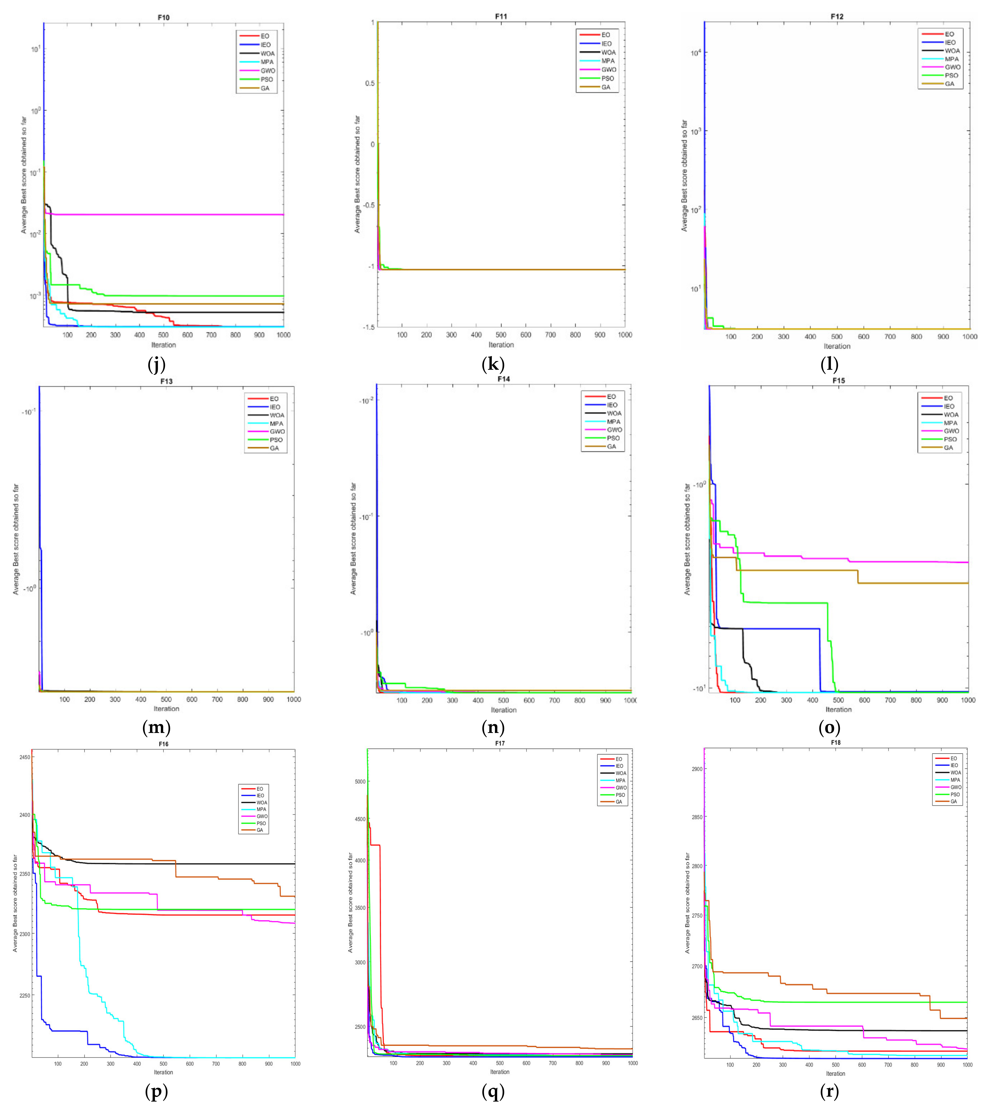
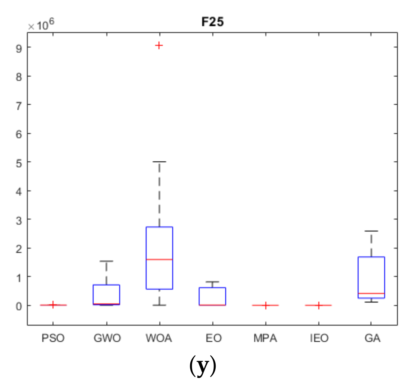
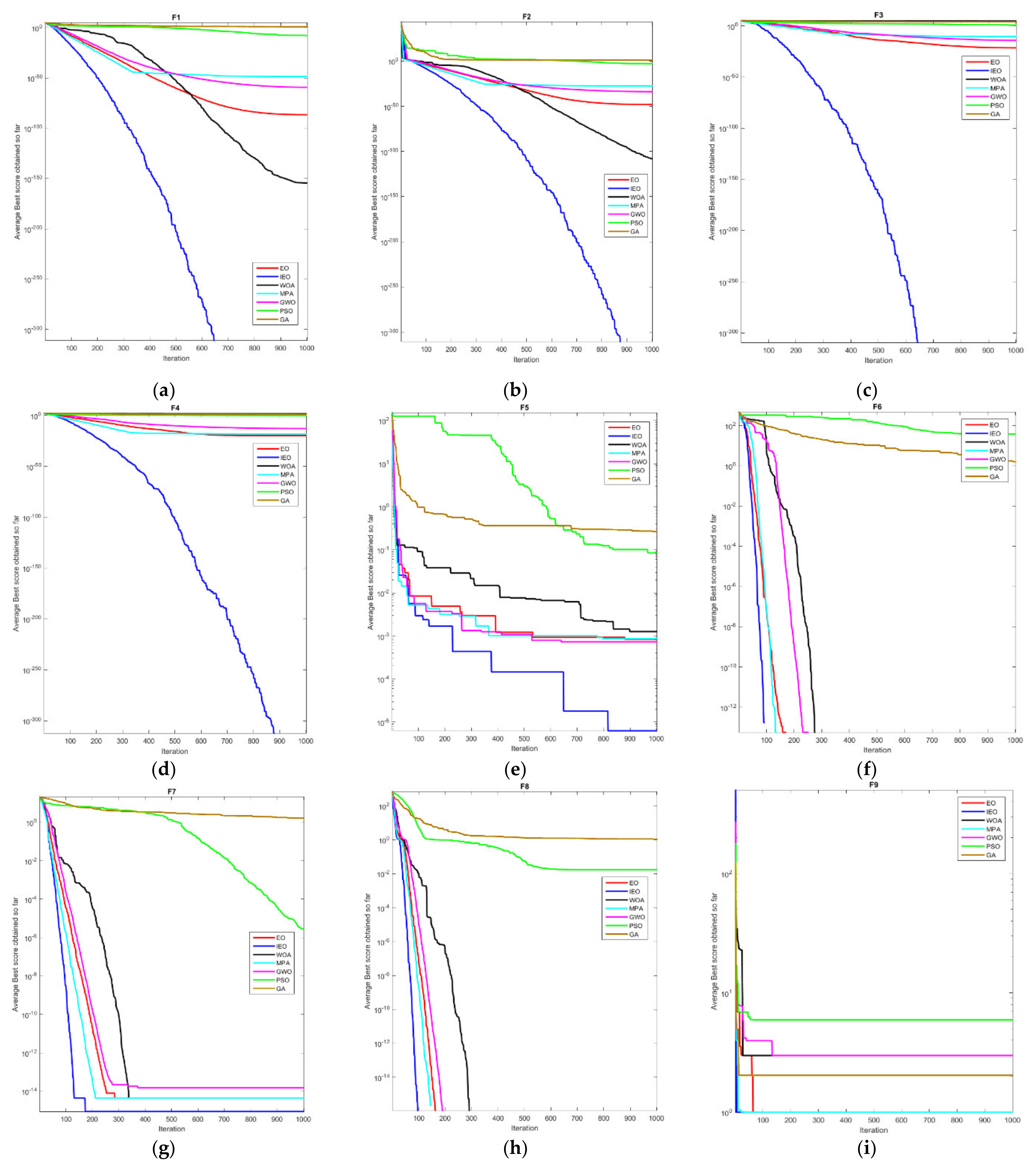
2.3.2. Benchmark Test Functions

Currently, the parameter settings of these 25 standard test functions have been widely adopted to verify meta-heuristics. In general, it is difficult for an algorithm to fit all test functions. Therefore, the 25 test functions selected are different. In this way, the experimental results can better reflect the capability of optimization for the algorithm.

The five high-dimensional unimodal test functions ($F_1(x)$~$F_5(x)$) have as few as one global optimal value but no local optimal value. Therefore, this function can be applied to test the algorithm for its capability of local search and convergence speed. In contrast to the high-dimensional unimodal function, the three high-dimensional multimodal test functions ($F_6(x)$~$F_8(x)$) have multiple local optimal values, thus making it more difficult for the algorithm to solve high-dimensional multimodal test functions than to solve unimodal functions. Thus, this function can be used to verify the algorithm for its capability of global search. The 7 fixed-dimensional multimodal functions ($F_9(x)$~$F_{15}(x)$) have multiple local extrema but the level of their dimensionality is lower as compared to high-dimensional multimodal functions. Therefore, the number of local extrema is relatively small. Similar to the high-dimensional multi-modal test function, the fixed-dimensional multi-modal test function can also be used to assess the algorithm for its performance in global search. To test its comprehensive capability, we added 10 composition functions of cec2017 [26]. In

Table 1. Description of benchmark functions.

Function	Dim	Range	${\mathit{f}}_{\mathbf{min}}$
$F_1(x)={\displaystyle \sum _{i=1}^n{x}_i^2}$	30	[−100, 100]	0
$F_2(x)={\displaystyle \sum _{i=1}^n\left|x_i\right|}+{\displaystyle \prod _{i=1}^n\left|x_i\right|}$	30	[−10, 10]	0
$F_3(x)={\displaystyle \sum _{i=1}^n{\left({\displaystyle \sum _{j-1}^i{x}_j}\right)}^2}$	30	[−100, 100]	0
$F_4(x)=\underset{i}{\max }\left\{\left|x_i\right|,\hspace{1em}1\le i\le n\right\}$	30	[−100, 100]	0
$F_5(x)={\displaystyle \sum _{i=1}^{n}i{x}_i^4}+\mathrm{random}[0,1)$	30	[−1.28, 1.28]	0
$F_6(x)={\displaystyle \sum _{i=1}^n\left[x_i^2-10\cos \left(2\pi x_i\right)+10\right]}$	30	[−5.12, 5.12]	0
$F_7(x)=-20\exp \left(-0.2\sqrt{\frac{1}{n}{\displaystyle \sum _{i=1}^n{x}_i^2}}\right)-\exp \left(\frac{1}{n}{\displaystyle \sum _{i=1}^n\cos \left(2\pi x_i\right)}\right)+20+e$	30	[−32, 32]	0
$F_8(x)=\frac{1}{4000}{\displaystyle \sum _{i=1}^n{x}_i^2}-{\displaystyle \prod _{i=1}^n\cos \left(\frac{x_i}{\sqrt{i}}\right)}+1$	30	[−600, 600]	−418.9829 × 5
$F_{\begin{array}{l}9\\ \end{array}}(x)={\left(\frac{1}{500}+{\displaystyle \sum _{j=1}^{25}}\frac{1}{j+{\displaystyle {\sum }_{i=1}^2}{\left(x_i-a_{ij}\right)}^6}\right)}^{-1}$	2	[−65, 65]	1
$F_{10}(x)={\displaystyle \sum _{i=1}^{11}{\left[a_i-\frac{x_1\left(b_i^2+b_i{x}_2\right)}{b_i^2+b_i{x}_3+x_4}\right]}^2}$	4	[−5, 5]	0.00030
$F_{11}(x)=4x_1^2-2.1x_1^4+\frac{1}{3}{x}_1^6+x_1{x}_2-4x_2^2+4x_2^4$	2	[−5, 5]	−1.0316
$\begin{array}{l}{F}_{12}(x)=\left[1+{\left(x_1+x_2+1\right)}^2\left(19-14x_1+3x_1^2-14x_2+6x_1{x}_2+3x_2^2\right)\right]\\ \times \left[30+{\left(2x_1-3x_2\right)}^2\times \left(18-32x_1+12x_1^2+48x_2-36x_1{x}_2+27x_2^2\right)\right]\end{array}$	2	[−2, 2]	3
$F_{13}(x)=-{\displaystyle \sum _{i=1}^4}{c}_i\exp \left(-{\displaystyle \sum _{j=1}^3}{a}_{ij}{\left(x_j-p_{ij}\right)}^2\right)$	3	[1, 3]	−3.86
$F_{14}(x)=-{\displaystyle \sum _{i=1}^4}{c}_i\exp \left(-{\displaystyle \sum _{j=1}^6}{a}_{ij}{\left(x_j-p_{ij}\right)}^2\right)$	6	[0, 1]	−3.32
$F_{15}(x)=-{\displaystyle \sum _{i=1}^{10}}{\left[\left(X-a_i\right){\left(X-a_i\right)}^T+c_i\right]}^{-1}$	4	[0, 10]	−10.5363
$F_{16}(x)=Composition Function 1 \left(N=3\right)$	30	${\left[-100,\hspace{0.33em}100\right]}^D$	0
$F_{17}(x)=Composition Function 2 \left(N=3\right)$	30	${\left[-100,\hspace{0.33em}100\right]}^D$	0
$F_{18}(x)=Composition Function 3 \left(N=4\right)$	30	${\left[-100,\hspace{0.33em}100\right]}^D$	0
$F_{19}(x)=Composition Function 4 \left(N=4\right)$	30	${\left[-100,\hspace{0.33em}100\right]}^D$	0
$F_{20}(x)=Composition Function 5 \left(N=5\right)$	30	${\left[-100,\hspace{0.33em}100\right]}^D$	0
$F_{21}(x)=Composition Function 6 \left(N=5\right)$	30	${\left[-100,\hspace{0.33em}100\right]}^D$	0
$F_{22}(x)=Composition Function 7 \left(N=6\right)$	30	${\left[-100,\hspace{0.33em}100\right]}^D$	0
$F_{23}(x)=Composition Function 8 \left(N=6\right)$	30	${\left[-100,\hspace{0.33em}100\right]}^D$	0
$F_{24}(x)=Composition Function 9 \left(N=3\right)$	30	${\left[-100,\hspace{0.33em}100\right]}^D$	0
$F_{25}(x)=Composition Function 10 \left(N=3\right)$	30	${\left[-100,\hspace{0.33em}100\right]}^D$	0

, Dim indicates the dimension of the standard test function, f_min represents the theoretical optimal value of the standard test function, and the range means the range of search space, N means the number of basic functions.

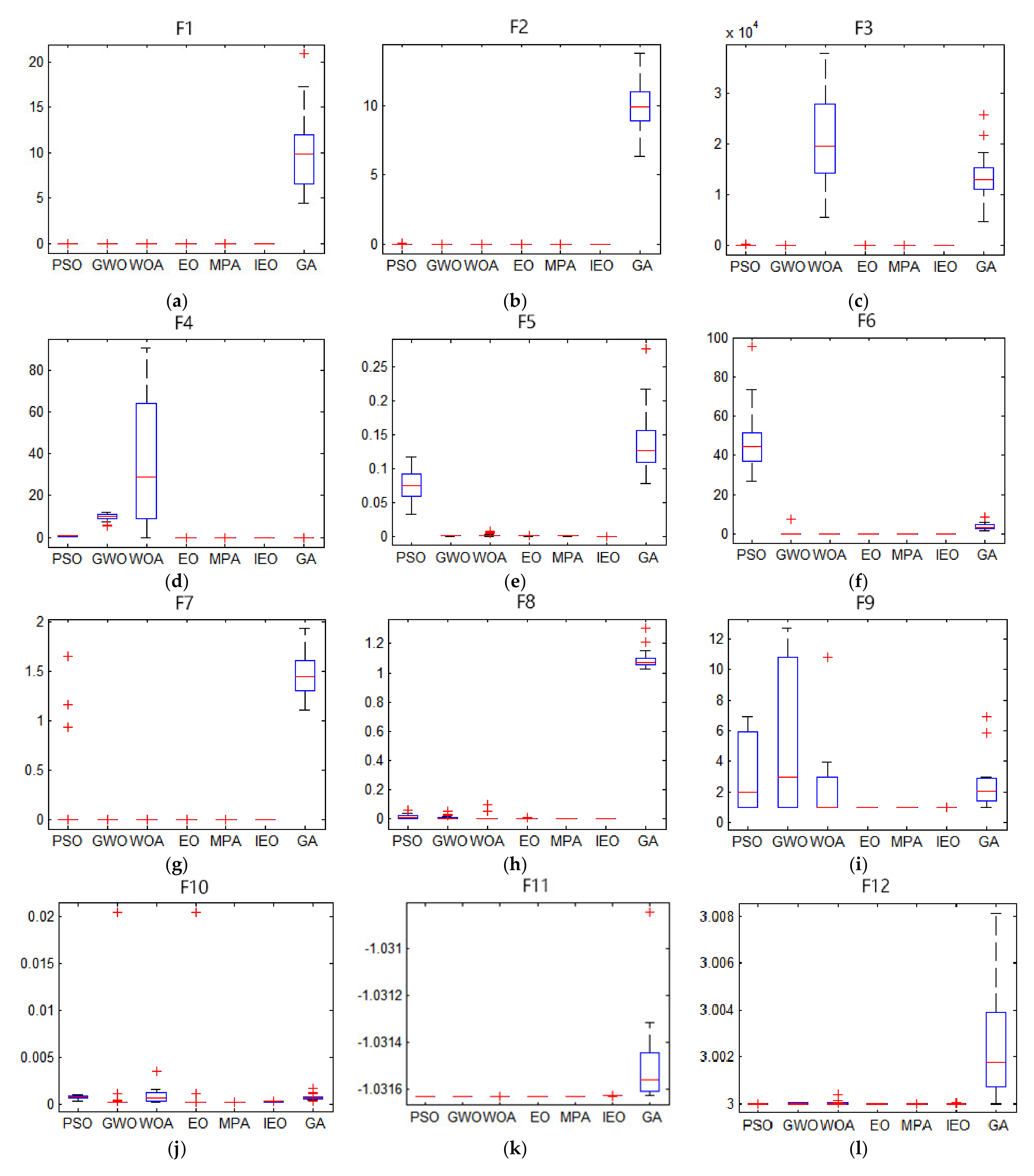
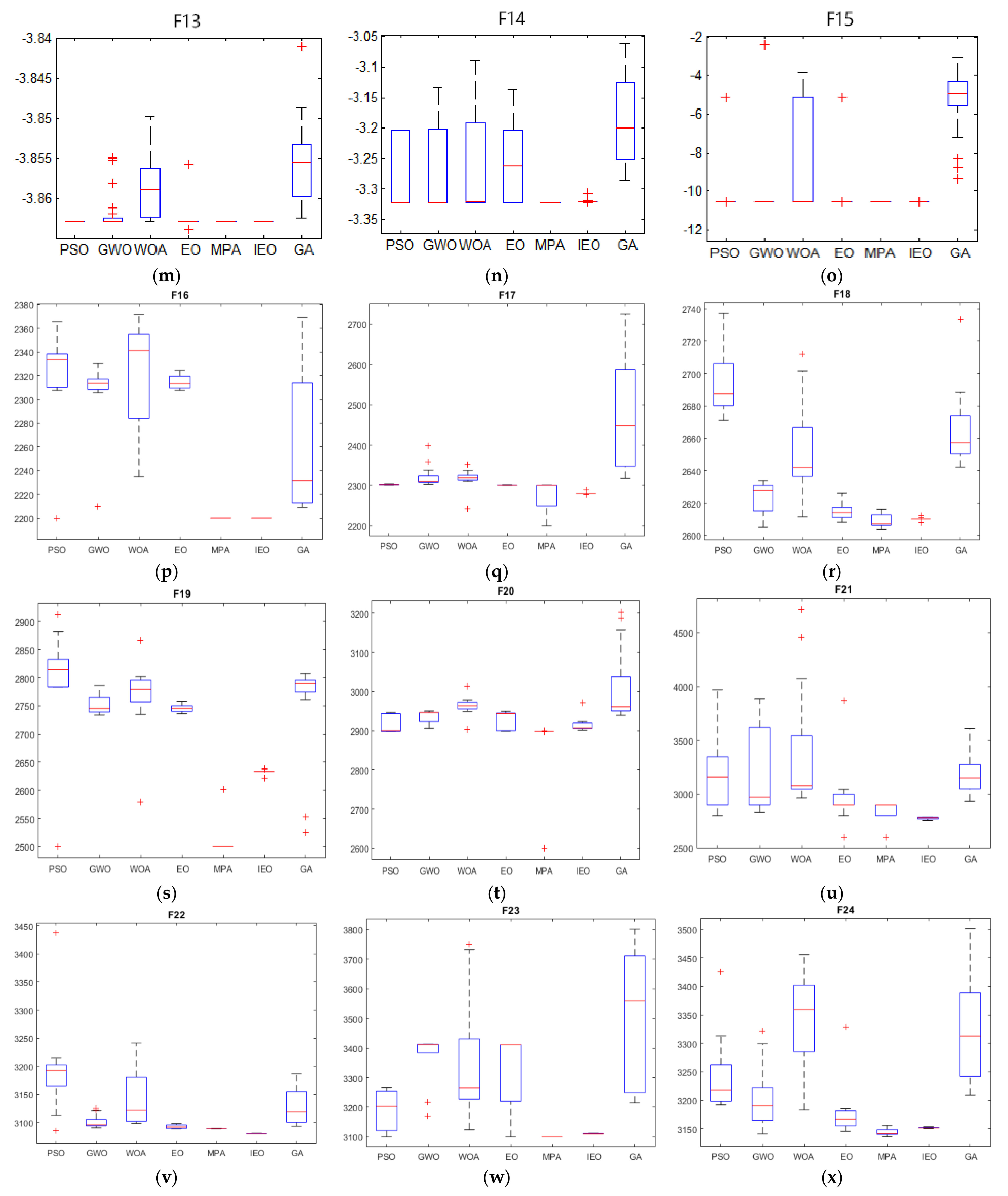
2.3.3. Experimental Results and Analysis

In this section, comparative numerical optimization experiments are conducted on EO, WOA, MPA, GWO, PSO, GA, and IEO, respectively. The convergence curve is presented in Figure A1, and the stability curve of each group optimization algorithm is presented in Figure A2. The test results of the unimodal function, high-dimensional multimodal function, fixed-dimensional multimodal function and composition functions are listed in

Table A1. Optimization results and comparison for functions.

	Function		IEO	EO	WOA	MPA	GWO	PSO	GA
Unimodal Benchmark Functions	F1	Ave	0.00 × 10+00	2.45 × 10−85	1.41 × 10−30	3.27 × 10−21	1.07 × 10−58	0.32 × 10+00	0.55 × 10+00
		Std	0.00 × 10+00	9.08 × 10−85	4.91 × 10−30	4.61 × 10−21	2.77 × 10−58	0.21 × 10+00	1.23 × 10+00
	F2	Ave	0.00 × 10+00	2.91 × 10−48	1.06 × 10−21	0.07 × 10+00	1.36 × 10−34	1.04 × 10+00	0.01 × 10+00
		Std	0.00 × 10+00	2.92 × 10−48	2.39 × 10−21	0.11 × 10+00	1.40 × 10−34	0.46 × 10+00	0.01 × 10+00
	F3	Ave	0.00 × 10+00	1.77 × 10−21	5.39 × 10−07	2.78 × 10+02	9.25 × 10−16	8.14 × 10+01	8.46 × 10+02
		Std	0.00 × 10+00	8.45 × 10−21	2.93 × 10−06	4.00 × 10+02	2.44 × 10−15	2.13 × 10+01	1.62 × 10+02
	F4	Ave	0.00 × 10+00	2.84 × 10−21	0.73 × 10−01	6.78 × 10+00	1.84 × 10−14	1.51 × 10+00	4.56 × 10+00
		Std	0.00 × 10+00	9.26 × 10−21	0.40 × 10+00	2.94 × 10+00	3.40 × 10−14	0.22 × 10+00	0.59 × 10+00
	F5	Ave	6.70 × 10−05	0.00 × 10+00	0.00 × 10+00	0.00 × 10+00	0.09 × 10+00	0.07 × 10+00	0.11 × 10+00
		Std	0.00 × 10+00	0.00 × 10+00	0.00 × 10+00	0.00 × 10+00	0.03 × 10+00	0.01 × 10+00	0.04 × 10+00
Multimodal Benchmark Functions	F6	Ave	0.00 × 10+00	0.00 × 10+00	0.00 × 10+00	0.00 × 10+00	0.00 × 10+00	4.84 × 10+01	0.00 × 10+00
		Std	0.00 × 10+00	0.00 × 10+00	0.00 × 10+00	0.00 × 10+00	0.00 × 10+00	3.44 × 10+00	3.97 × 10+00
	F7	Ave	8.84 × 10−16	5.15 × 10−15	7.40 × 10+00	9.69 × 10−12	0.00 × 10+00	1.20 × 10+00	0.18 × 10+00
		Std	0.00 × 10+00	1.45 × 10−15	9.90 × 10+00	6.13 × 10−12	0.00 × 10+00	0.73 × 10+00	0.15 × 10+00
	F8	Ave	0.00 × 10+00	0.00 × 10+00	0.00 × 10+00	0.00 × 10+00	0.60 × 10+00	0.01 × 10+00	0.66 × 10+00
		Std	0.00 × 10+00	0.00 × 10+00	0.00 × 10+00	0.00 × 10+00	0.09 × 10+00	0.01 × 10+00	0.19 × 10+00
Fifixed-Dimenstion Multimodal Benchmark Functions	F9	Ave	1.00 × 10+00	1.00 × 10+00	2.11 × 10+00	1.00 × 10+00	0.16 × 10+00	2.18 × 10+00	1.00 × 10+00
		Std	2.12 × 10−17	1.11 × 10−16	2.50 × 10+00	2.47 × 10−16	0.84 × 10+00	2.01 × 10+00	8.84 × 10−12
	F10	Ave	3.58 × 10−04	3.69 × 10−49	0.00 × 10+00	3.07 × 10−04	1.62 × 10−04	5.61 × 10−04	2.69 × 10−03
		Std	1.54 × 10−04	2.36 × 10−04	0.00 × 10+00	4.09 × 10−15	3.33 × 10−04	4.38 × 10−04	4.84 × 10−03
	F11	Ave	−1.03 × 10+00	−1.03 × 10+00	−1.03 × 10+00	−1.03 × 10+00	−1.03 × 10+00	−1.03 × 10+00	−1.03 × 10+00
		Std	5.63 × 10−06	2.04 × 10+16	4.2 × 10−07	4.46 × 10−01	5.46 × 10−09	6.64 × 10−16	2.39 × 10−08
	F12	Ave	3.00 × 10+00	3.00 × 10+00	3.00 × 10+00	3.00 × 10+00	3.00 × 10+00	3.00 × 10+00	3.00 × 10+00
		Std	5.95 × 10−17	4.96 × 10−16	4.22 × 10−15	1.95 × 10−15	2.29 × 10−02	1.38 × 10−15	2.45 × 10−07
	F13	Ave	−3.86 × 10+00	−3.86 × 10+00	−3.85 × 10+00	−3.86 × 10+00	0.51 × 10+00	−3.86 × 10+00	−3.86 × 10+00
		Std	3.17 × 10−16	2.15 × 10−15	0.00 × 10+00	2.42 × 10−15	2.73 × 10−15	2.68 × 10−15	2.85 × 10−8
	F14	Ave	−3.32 × 10+00	-−3.28 × 10+00	−2.98 × 10+00	−3.32 × 10+00	−2.84×10+00	−3.26 × 10+00	−3.27 × 10+00
		Std	1.59 × 10−15	0.06 × 10+00	0.38 × 10+00	1.14 × 10−11	4.68 × 10−2	6.05 × 10−2	5.99 × 10−2
	F15	Ave	−1.05 × 10+1	−10.27 × 10+00	−9.34 × 10+00	−1.05 × 10+1	−7.11 × 10+00	−7.25 × 10+00	−7.77 × 10+00
		Std	1.92 × 10−07	1.48 × 10+00	2.41 × 10+00	3.89 × 10−11	3.11 × 10+00	3.66 × 10+00	3.73 × 10+00
Composition Functions	F16	Ave	2.20 × 10+03	2.30 × 10+03	2.33 × 10+03	2.20 × 10+03	2.31 × 10+03	2.32 × 10+03	2.28 × 10+03
		Std	6.54 × 10−07	4.13 × 10+01	4.34 × 10+01	8.66 × 10−06	2.28 × 10+01	6.34 × 10+01	5.84 × 10+01
	F17	Ave	2.28 × 10+3	2.30 × 10+03	2.36 × 10+03	2.28 × 10−06	2.31 × 10+03	2.37 × 10+03	2.41 × 10+03
		Std	0.54 × 10+00	0.35 × 10+00	1.43 × 10+02	3.38 × 10+01	8.52 × 10+00	3.20 × 10+02	1.00 × 10+02
	F18	Ave	2.61 × 10+03	2.62 × 10+03	2.65 × 10+03	2.61 × 10+03	2.62 × 10+03	2.71 × 10+03	2.65 × 10+03
		Std	3.55 × 10+00	8.76 × 10+00	2.88 × 10+01	5.06 × 10+00	1.04 × 10+01	4.18 × 10+01	1.28 × 10+01
	F19	Ave	2.63 × 10+02	2.74 × 10+03	2.76 × 10+03	2.51 × 10+03	2.75 × 10+03	2.77 × 10+02	2.79 × 10+03
		Std	5.13 × 10+00	4.30 × 10+00	6.11 × 10+01	3.58 × 10+01	1.40 × 10+01	1.16 × 10+02	2.31 × 10+01
	F20	Ave	2.91 × 10+03	2.92 × 10+03	2.95 × 10+03	2.88 × 10+03	2.94 × 10+03	2.90 × 10+03	2.99 × 10+02
		Std	2.29 × 10+01	2.39 × 10+02	2.36 × 10+01	2.09 × 10+01	2.68 × 10+01	8.60 × 10+01	8.07 × 10+01
	F21	Ave	2.78 × 10+03	3.03 × 10+03	3.60 × 10+03	2.79 × 10+03	3.23 × 10+03	3.08 × 10+03	3.20 × 10+03
		Std	5.11 × 10+01	3.07 × 10+02	6.33 × 10+02	1.10 × 10+02	4.32 × 10+02	3.57 × 10+02	2.17 × 10+02
	F22	Ave	3.08 × 10+03	3.09 × 10+03	3.13 × 10+03	3.09 × 10+03	3.10 × 10+03	3.16 × 10+03	3.14 × 10+03
		Std	0.33 × 10+00	6.52 × 10+00	4.27 × 10+01	0.22 × 10+00	2.11 × 10+01	7.44 × 10+01	3.53 × 10+01
	F23	Ave	3.11 × 10+03	3.32 × 10+03	3.41 × 10+03	3.12 × 10+03	3.34 × 10+03	3.19 × 10+03	3.62 × 10+03
		Std	5.57 × 10−05	1.41 × 10+02	1.77 × 10+02	5.00 × 10−05	9.99 × 10+01	6.07 × 10+01	2.02 × 10+02
	F24	Ave	3.15 × 10+03	3.18 × 10+03	3.36 × 10+03	3.14 × 10+03	3.22 × 10+03	3.26 × 10+03	3.30 × 10+03
		Std	3.14 × 10+00	3.47 × 10+01	1.12 × 10+02	8.63 × 10+00	5.49 × 10+01	8.77 × 10+01	8.67 × 10+01
	F25	Ave	4.73 × 10+03	3.35 × 10+05	9.75 × 10+05	3.40 × 10+03	1.03 × 10+06	1.08 × 10+04	1.39 × 10+06
		Std	3.51 × 10+01	4.11 × 10+05	8.97 × 10+05	3.51 × 10+01	1.09 × 10+06	4.96 × 10+03	1.10 × 10+06

, where Ave and Std represent the average solution in 30 independent experiments and the standard deviation of the results in 30 runs, respectively.

As shown in Figure A1, the convergence speed of IEO on $F_1(x)$~$F_5(x)$ is significantly higher when compared with other algorithms and it achieves higher accuracy of convergence. Besides, the convergence of each function is relatively slow, and the IEO convergence value is shown to be the best, suggesting that the IEO is less prone to the local optimum. In general, when the high-dimensional unimodal function is tested, the IEO algorithm demonstrates its superior and consistent performance, implying its effectiveness in solving the high dimensionality of space. On $F_6(x)$~$F_8(x)$, the convergence speed of IEO is the highest, and the accuracy of convergence is improved, suggesting that IEO has a better ability to jump out of the local optimum than other algorithms. Compared with other algorithms, it can be seen from the average (Ave) and standard deviation (Std) that IEO performs best and is most stable. Overall, the performance of the IEO algorithm in solving the high-dimensional multi-peak test function shows higher stability than other algorithms, which evidences its strong capability of global search. On $F_9(x)$~$F_{15}(x)$, in the first five functions, IEO is not only reflected in the fastest convergence speed, but also the higher convergence accuracy. While on $F_{15}(x)$, despite the slow convergence of IEO, it jumped out of the local optimum in the later stage and found the optimum value which is closer to the theory. In general, the capability of IEO to jump out of the local optimal value is better than that of other algorithms for the fixed-dimensional multi-modal function. Thus, the algorithm is verified as effective and stable. On $F_{16}(x)$~$F_{25}(x)$, Overall, the convergence speed of IEO is faster than that of EO, and compared with other algorithms, the convergence speed of IEO has certain advantages. Among them, $F_{16}(x)$, $F_{18}(x)$, $F_{21}(x)$ and $F_{23}(x)$ converge the fastest and obtain the optimal value. As shown in Table A1, on $F_1(x)$~$F_5(x)$, the IEO algorithm outperforms other algorithms. In these five test functions, IEO produces better results than other algorithms regardless of the average value or the standard deviation, and the accuracy of convergence is significantly improved relative to other algorithms. Moreover, in the tests in four of the functions, IEO achieved the ideal optimal value of 0 every time. The variance of the IEO algorithm is considerably smaller as compared to other algorithms, which indicates the stability of the IEO algorithm. On the high-dimensional multimodal test functions $F_6(x)$~$F_8(x)$, IEO outperforms other algorithms to a significant extent. Compared with other algorithms, IEO performs more consistently with the smallest average and standard deviation. Notably, it achieves the theoretical optimal value of 0 on $F_6(x)$ and $F_8(x)$. On fixed-dimensional multimodal functions ($F_9(x)$~$F_{15}(x)$), the data comparison of all algorithms to optimize the fixed-dimensional multimodal function is performed. According to the comparison of the mean and standard deviation in the table, IEO performs better in mean and standard deviation on the test functions of $F_9(x)$, $F_{12}(x)$, and $F_{13}(x)$, while MPA performs best in average and standard deviation on $F_{10}(x)$, followed by IEO. On $F_{11}(x)$, the average and standard deviation of IEO are not as satisfactory as the four functions of MPA, GWO, PSO and GA. On $F_{14}(x)$, EO has achieved the best average and standard deviation, followed by IEO. On $F_{15}(x)$, IEO and MPA have achieved the best average and standard deviation together. As a whole, IEO shows stronger capabilities of global search in fixed-dimensional multi-modal functions. On $F_{16}(x)$~$F_{25}(x)$, $F_{16}(x)$, $F_{18}(x)$, $F_{21}(x)$ and $F_{22}(x)$ all achieved the minimum value. In the remaining functions, IEO performed better than EO, indicating that the IEO improvement strategy was successful. It shows that IEO has a significant improvement over EO in solving composition functions, and has a great advantage over other algorithms, and ranks second in most of the functions. Figure A2 shows the test result block diagram of the selected function. In the experiment, box plots are used to indicate the distribution of the results for each function after 30 independent tests to demonstrate the stability of IEO and other algorithms in a more intuitive way. The numerical distribution of the selected function is selected from the test functions. IEO exhibits outstanding stability in all functions, which allows it to outperform other algorithms. More specifically, its bottom edge, top edge, and median value of the same function are superior or inferior to other algorithms.

In general, the IEO optimization algorithm outperforms other algorithms in optimization speed, accuracy and stability.

3. LSTM Model Optimization by Improved IEO Algorithm

Time series data are everywhere, and prediction is an eternal topic for human beings. Gooijer and Hyndman highlight researched published in the International Institute of Forecasters (IIF) and key publications in other journals [27]. From the early traditional autoregressive integrated moving average (ARIMA) linear model to various nonlinear models (e.g., SETAR model). Due to increased computational power and electronic storage capacity, nonlinear forecasting models have grown in a spectacular way and received a great deal of attention during the last decades. The neural networks (NN) model is a prominent example of such nonlinear and nonparametric models that do not make assumptions about the parametric form of the functional relationship between the variables. Several studies have been done relating to the application of NN, such as Caraka and Chen used vector autoregressive (VAR) to improve NN for space-time pollution date forecasting modeling [28], then they used VAR-NN-PSO model to predicting PM_2.5 in air [29]. Suhartono and Prastyo applied Generalized Space-Time Autoregressive (GSTAVR) to FFNN for forecasting oil production [30]. In recent years, types of recurrent neural networks (RNN) have been frequently employed for forecasting tasks and have shown promising reslts. This is mainly due to RNNs having the ability to persist information about previous time steps and being able to use that information when processing the current time step. Due to vanishing gradients, RNN is unable to persist long-term dependencies. A long short term memory (LSTM) network is a type of RNN that was introduced to persist long term dependencies [31]. By comparing LSTM with a random forest, a standard deep net, and a simple logistic regression in the large-scale financial market prediction task. It is proved that LSTM performed better than others and was a method naturally suitable for this field [32]. By comparing LSTM with the Prophet model proposed by Facebook, the result showed LSTM performs better on minimum air temperature [33]. ChihHung and Yu-Feng proposed a new forecasting framework with the LSTM model to forecasting bitcoin daily prices. The results revealed its possible applicability in various cryptocurrencies prediction [34]. Helmini and Jihan adopted a special variant LSTM with peephole connections for the sales forecasting tasks, proved that the initial LSTM and improved LSTM both outperform two machine learning models (extreme gradient boosting (XGB) and random forest regressor (RFR)) [35]. To enhance the performance of the LSTM model, Gers and Schmidhuber proposed a novel adaptive “forget gate” that enables an LSTM cell to learn to reset itself at appropriate times [36], Karim and Majumdar added the attention model to detect regions of the input sequence that contribute to the class label through the context vector [37]. Saeed and Li proposed a hybrid model called BLSTM, constructing quality intervals based on the high-quality principle, presented excellent prediction performance [38]. Venskus and Treigys described two methods—the LSTM prediction region learning and the wild bootstrapping for estimation of prediction regions—and the expected results have been achieved when it is used for abnormal marine traffic detection [39]. In order to strengthen the early diagnosis of cardiovascular disease, Zheng and Chen presented an arrhythmia classification method that combines 2-D CNN and LSTM and uses ECG images as the input data for the model [40]. Currently, the most mainstream method for time series forecasting would be LSTM and its variants.

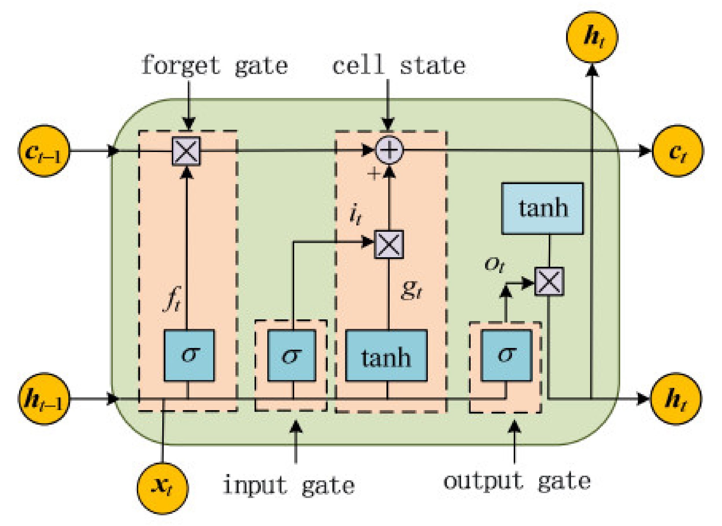
3.1. Basic Model of LSTM

The LSTM model introduces a gating unit into its network topology for gaining control on the degree of impact of current information on the previous information, thus endowing the model with a longer “memory function”. It is made suitable for solving long-term nonlinear sequence forecasting problems. The LSTM network structure consists of input gates, forget gates, output gates, and unit states. The basic structure of the network is illustrated in Figure 2.

LSTM is a purpose-built recurrent neural network. Not only does the design of the “gate” structure avoid the gradient disappearance and gradient explosion caused by traditional recurrent neural networks, it is also effective in learning long-term dependency. Therefore, the LSTM model with memory function shows a clear advantage in dealing with the problems arising from the prediction and classification of time series.

Let the input sequence be $\left(x_1,x_2,\cdots ,x_T\right)$, and the hidden layer state be $\left(h_1,h_2,\cdots ,h_T\right)$. Then, at time t:

$$f_t=\sigma \left(W_f{h}_{t-1}+U_f{x}_t+b_f\right)$$

(16)

$$i_t=\sigma \left(W_i{h}_{t-1}+U_i{x}_t+b_i\right)$$

(17)

$$g_t=tanh\left(W_C{h}_{t-1}+U_C{x}_t+b_C\right)$$

(18)

$$C_t=f_t\ast C_{t-1}+i_t\ast g_t$$

(19)

$$o_t=\sigma \left(W_o{h}_{t-1}+U_o{x}_t+b_o\right)$$

(20)

$$h_t=o_t\ast tanh\left(C_t\right)$$

(21)

where, $x_t$ represents the input vector of the LSTM cell; $h$ indicates the cell output vector; $f_t$, $i_t$, and ${ \mathrm{o}}_t$ refer to the forget gate, input gate, output gate, respectively; $C_t$ denotes the status of the cell unit; $t$ stands for the time; $\sigma$ and $tanh$ represent the activation functions; $W$ and $b$ denote the weight and deviation matrix, respectively. $U$ stands for the input weight matrix.

The key to LSTM lies in the cell state $C_t$. It maintains the memory of the unit state at time $t$, and adjusts it through the forget gate $f_t$ and input gate $i_t$. The purpose of the forget gate is to make the cell remember or forget its previous state $C_{t-1}$. The input gate is purposed to allow incoming signals to update the unit state or prevent it. The output gate aims to control the output of the unit state $C_t$ and then transmit it to the next cell. The internal structure of the LSTM unit is comprised of multiple perceptrons. In general, backpropagation algorithms are the most commonly used training method.

The LSTM neural network framework applied in the design of this paper involves one input layer, three hidden layers (64 neurons in the first layer, 16 neurons in the second layer, and 50 neurons in the third fully connected layer), and one output layer (two neuron output). Using the Adam optimizer, the learning rate is 0.01, the loop is executed 30 times, and the batch size is 256.

3.2. LSTM Based on Improved EO

As mentioned above, the parameters of the LSTM-based model are set manually, which however affects the outcome of the prediction made using the model. Thus, an improved EO-LSTM model is proposed in this paper. The main purpose of doing so is to optimize the relevant parameters of the LSTM through the excellent parameter optimization capabilities of the above-mentioned IEO algorithm for the improved outcome of prediction for the LSTM. In order to ensure the objectivity of the experiment, the LSTM model structure is fixed (the number of nodes in each layer does not modified), The modeling process of the IEO-LSTM model is detailed as follows.

(1)

The relevant parameters are initialized. The parameters of the IEO algorithm are initialized, including: population size, fitness function, are free parameter assignment. The parameters of the LSTM algorithm are initialized by setting the time window, the initial learning rate, the number of initial iterations, and the size of the packet. In this paper, the error is treated as a fitness function, which is expressed as follows:

$$fitness=1-\mathrm{acc}(f;D)=1-\frac{1}{m}{\displaystyle \sum _{i=1}^{m}I}\left(f\left(x_i\right)=y_i\right)$$

(22)

where D represents the training set, m denotes the number of samples in the training set, $f\left(x_i\right)$ indicates the predicted sample label, $y_i$ means the original sample label, and $I(f\left(x_i\right)=y_i)$ is a function. If $f\left(x_i\right)=y_i$, $I(f\left(x_i\right)=y_i)$ = 1; otherwise, $I(f\left(x_i\right)=y_i)$ = 0.

(2)

The LSTM parameters are set as required to form the corresponding particles. The particle structure is ($alpha$, $num\_epochs$, $batch\_size$). Among them, $alpha$ represents the LSTM learning rate, $num\_epochs$ indicates the number of iterations, $batch\_size$ suggests the size of the bag. The particles mentioned above are the objects of IEO optimization.

(3)

The concentration is updated according to Equation (15). According to the newly-obtained concentration, calculate the fitness value and then update the individual optimal concentration and the global optimal concentration of the particles.

(4)

If the number of iterations reaches the maximum number of times of iteration, that is, 30, the LSTM model trained on the optimal particles will output the prediction value; otherwise, return to step (3) for continued iteration.

(5)

The optimal parameters are substituted into the LSTM model, for constructing obtaining the IEO-LSTM model.

The pseudo-code of the IEO-LSTM on oil prediction algorithm is shown in Algorithm 2.

Algorithm 2 Pseudo-code of the IEO-LSTM on oil prediction.

Input:

Training samples set: trainset_input, trainset_output

LSTM initialization parameters

Output: IEO-LSTM model

1. Initialize the LSTM model:

assign parameters para = [lr,epoch,batch_size] = [0.01,100,256];

loss = categorical_crossentropy, optimizer = adam

2. Set IEO equalization parameters and Import trainset to Optimization:     Parameters:para = [lr,epoch,batch_size]     Ll para = [0.001,1, 1, 1, 1, 1];        % Set lower limit for merit search     Ul para = [0.01, 100,256, 100, 100,100];    % Set the upper limit of merit seeking       IEO_para = [ll,ul,trainset_input, trainset_output, num_epoch = 30];       Get_fitness_position ((IEO)) = length(find((trainset_output - LSTM(trainset-             input)~ = 0))/length(trainset_output);             % Find the best Concentration to minimize the LSTM error rate return para_best to LSTM model; save (‘IEO-LSTM.mat’,’LSTM’)

3.3. Actual Application in Oil Layer Prediction

3.3.1. Design of Oil Layer Prediction System

In respect of oil logging, reservoir prediction is regarded as crucial for improving the accuracy of oil layer prediction. Herein, we apply IEO-LSTM to oil logging and verify the effectiveness of this algorithm by using oil data provided by three oil fields.

Figure 3 shows the block diagram of the oil layer prediction system based on IEO-LSTM.

The oil layer prediction mainly includes the following processes:

(1)

Data acquisition and preprocessing

In practice, the logging data is classified into two categories after being collected. On the one hand, labeled data as obtained through core sampling and laboratory analysis is generally used as a training set. On the other hand, the unlabeled logging data is treated as the test set. The data pre-processing mainly includes denoising process, normalization process, etc.

Besides, due to the different dimensions of each attribute and value range, these data need to be normalized in the first place, so that the sample data ranges between [0,1]. The normalized logging data are then trained and tested. The formula for sample normalization is expressed as follows:

$$\overline{x}=\frac{\left(x-x_{\min }\right)}{x_{\max }-x_{\min }}$$

(23)

where, $x\in \left[x_{\min },x_{\max }\right]$; $x_{\min }$ represents the minimum value of the attributes of the data sample, and $x_{\max }$ refers to the maximum value of the attribute of the data sample.

(2)

Selection of sample set and attribute reduction

In the selection of the sample set, the selection of the sample set for training is supposed not only to be complete and comprehensive but also to be closely related to the evaluation of the oil. Moreover, the degree to which the prediction of oil can be made varies due to the different attributes of oil logging. In general, there are dozens of logging condition attributes in logging data but not all of them play a decisive role, which makes it necessary to perform attribute reduction. In this paper, the discretization algorithm based on the inflection point is applied and then the reduction method based on the attribute dependence is applied to reduce the logging attributes [41].

(3)

IEO-LSTM modeling

First of all, the LSTM model is established, the training set information is inputted after attribute reduction, and The IEO algorithm is used to find the optimal combination of parameters for the LSTM model to obtain a high-precision IEO-LSTM prediction model.

(4)

Prediction

The trained IEO-LSTM model is used to perform prediction and output the results. Among them, before the test set is inputted into the IEO-LSTM model, the reduced test set must be obtained according to the sample attribute reduction result for normalization according to the normalization principle of sample training.

The pseudo-code of the oil layer prediction system based on IEO-LSTM is shown in Algorithm 3.

Algorithm 3 Pseudo-code of the oil prediction system based on IEO-LSTM.

Input:

Training samples set: trainset_input, trainset_output, testset

Test samples set: testset

Output: Parameter optimization value Prediction results of the test samples set

1. Original data initialization, Divide the trainset and testset

2. Initialize the LSTM model:

assign parameters para = [lr,epoch,batch_size] = [0.01,100,256];

loss = categorical_crossentropy, optimizer = adama;

3. Set IEO equalization parameters and Import trainset to Optimization: 4. Set IEO equalization parameters and Import trainset to Optimization:    Parameters:para = [lr,epoch,batch_size]     ll =[0.001,1, 1];        % Set lower limit for merit search     ul = [0.01, 100, 256];      % Set the upper limit of merit seeking     para = IEO[ll,ul,trainset_input, trainset_output, num_epoch = 30];     Get_fitness_position ($\overrightarrow{C}$) = length(find((trainset_output—LSTM(trainset-         input)~ = 0))/length(trainset_output);         % Find the best Concentration to minimize the LSTM error rate return para_best to LSTM model; save (‘IEO-LSTM.mat’,’LSTM’); 5. Import test samples set to IEO-LSTM load(‘IEO-LSTM.mat’) predictset = IEO-LSTM(testset) return predictset

3.3.2. Practical Application

To verify the effectiveness and stability of the proposed IEO-LSTM model, we selected logging data from three actual oil wells for the experiment. And the prediction results are compared and evaluated with those of the LSTM, PSO-LSTM [42], GA-LSTM [43] and EO-LSTM models.

The logging data for the three selected actual wells were recorded as $o_1$, $o_2$ and $o_3$,

Table 2. Reduction results of logging data.

Well	Attributes
Original results ($o_1$)	GR,DT,SP,WQ,LLD,LLS,DEN,NPHI,PE,U,TH,K,CALI
Reduction results ($o_1$)	GR, DT,SP,LLD,LLS, DEN, K
Original results ($o_2$)	AC,CNL,DEN,GR,RT,RI,RXO,SP,R2M,R025,BZSP,RA2,C1,C2,CALI,RINC,PORT,VCL,VMA1,VMA6,RHOG,SW,VO,WO,PORE,VXO,VW,so,rnsy,rsly,rny,AC1
Reduction results ($o_2$)	AC,GR,RT,RXO,SP
Original results ($o_3$)	AC,CALI,GR,NG,RA2,RA4,RI,RM,RT,RXO,SP
Reduction results ($o_3$)	AC,NG,RI,SP
Decision attribute	where–1, 1 represents the dry layer and oil layer respectively.

shows the reduction results obtained after the attribute reduction process for the three wells. It can be seen from the table that there are various redundant condition attributes in the original data. After attribute reduction is performed through a rough set, those significant attributes can be selected, which is conducive to simplifying the complexity of the LSTM model. The data set division of three wells is shown in

Table 3. Data set partition details.

Well	Depth (m)	Training Set		Depth (m)	Test Set
		Oil Layer	Dry Layer		Oil Layer	Dry Layer
$o_1$	3150~3330	122	1319	3330~3460	115	925
$o_2$	1180~1255	65	496	1230~1300	40	360
$o_3$	1150~1250	65	736	1233~1260	104	112

. It can be seen from Table 3 that the oil layer and dry layer distribution range in the training set and test set.

Table 4. Value range of attributes in $o_1$.

Attributes	GR	DT	SP	LLD	LLS	DEN	K
Boundary	[6, 200]	[152, 462]	[−167, −68]	[0, 25000]	[0, 3307]	[1, 4]	[0, 5]

lists the value range of each attribute after $o_1$ attribute reduction. Among them, $GR$, $DT$, $SP$, $LLD$, $LLS$, $DEN$, and $K$ represent natural gamma, acoustic time difference, natural potential, deep lateral resistivity, shallow lateral resistivity, compensation density, and potassium, respectively. Besides,

Table 5. Value range of attributes in $o_2$.

Attributes	AC	GR	RT	RXO	SP
Boundary	[54, 140]	[27, 100]	[2, 90]	[1, 328]	[−32, −6]

shows the value range of each attribute after $o_2$ attribute reduction. Among them, $AC$, $RT$, and $RXO$ denote jet lag, intact formation resistivity, and flush zone resistivity, respectively.

Table 6. Value range of attributes in $o_3$.

Attributes	AC	NG	RI	SP
Boundary	[0, 571]	[0, 42]	[−1, 81]	[−50, 28]

lists the value range of each attribute after $o_3$ attribute reduction, where $NG$ and $RI$ represent neutron gamma and intrusion zone resistivity, respectively.

The logging curve is obtained after the normalization of the reduced attributes, as shown in Figure 4. The horizontal axis and the vertical axis indicate the depth and the standardized value, respectively.

In order to conduct comparative experiments better, the LSTM model, PSO-LSTM model, GA-LSTM model, and EO-LSTM model are established for comparison against the IEO-LSTM model. Then, these optimized classification models are applied to oil predict using the test set.

In addition to the prediction accuracy of the test set, the following performance indicators are defined to assess the performance of the prediction model:

$$\mathrm{MSE}=\frac{1}{m}{\displaystyle \sum }_{i=1}^m{\left(f\left(x_i\right)-y_i\right)}^2$$

(24)

$$RMSE=\sqrt{\frac{1}{m}\underset{i=1}{\overset{m}{{\displaystyle a}}}{\left(f\left(x_i\right)-y_i\right)}^2}$$

(25)

$$\mathrm{MAE}=\frac{1}{m}{\displaystyle \sum }_{i=1}^m\left|f\left(x_i\right)-y_i\right|$$

(26)

where, $f\left(x_i\right)$ and $y_i$ represent the predicted output value and the expected output value, respectively.

RMSE is applied to measure the deviation between the observed value and the true value. MAE is referred to as the average of absolute errors. If the RMSE and MAE are reduced, the performance of the algorithm model is improved. Therefore, RMSE is treated as a criterion applied to evaluate the accuracy of each algorithm model. MAE is often treated as the actual forecast and forecast error because it can better reflect the real state of the forecast value error.

For a comprehensive experimental comparison, the number of times of training is set to 30, based on which the average value of the performance indicators is calculated for each model.

Table 7. Prediction performance on $o_1$, $o_2$, $o_3$.

Optimization Algorithm	Oil	Learning Rate	Epochs	Batch Size	ACC	MSE	RMSE	MAE
LSTM	o1	0.01	100	256	0.8837	0.2049	0.4887	0.2341
	o2	0.01	100	256	0.8937	0.1765	0.0519	0.0826
	o3	0.01	100	256	0.9095	0.1561	0.4896	0.1971
PSO_LSTM	o1	0.0098	86	103	0.9025	0.1697	0.3925	0.1137
	o2	0.0011	42	154	0.9154	0.0937	0. 035	0.0985
	o3	0.003	52	75	0.8859	0.0952	0.3131	0.0933
GA_LSTM	o1	0.0082	20	200	0.9084	0.6732	0.8587	0.7368
	o2	0.0082	54	167	0.8979	0.0753	0.2853	0.0877
	o3	0.0038	29	176	0.9132	0.1368	0.3368	0.1404
EO_LSTM	o1	0.0089	28	163	0.9231	0.1481	0.2347	0.5442
	o2	0.0081	45	127	0.9183	0.0605	0.0375	0.0116
	o3	0.0049	56	155	0.9203	0.0795	0.2353	0.0793
IEO_LSTM	o1	0.0030	29	137	0.9433	0.1023	0.3781	0.4544
	o2	0.0082	43	109	0.9371	0.041	0.0212	0.0107
	o3	0.0027	53	128	0.9661	0.0323	0.2016	0.0571

shows the prediction ability of each model on the test set of three wells ($o_1$, $o_2$, $o_3$). On the whole, the prediction accuracy of IEO-LSTM is most satisfactory. Compared with other models, it performs better in each index, and the accuracy of it is about 5% higher than the original LSTM model on average.

4. Conclusions

In this paper, an improved equalization optimization algorithm is proposed, which applies chaos theory to initialize the population and relies on adaptive weights to enhance the capability of global and local search. Firstly, a total of 30 independent experiments are conducted on 25 benchmarks using six popular swarm intelligence algorithms. According to the experimental results, IEO achieves a significant improvement of convergence speed and convergence accuracy as compared to traditional EO. Compared with PSO, GA, MPA, WOA, and GWO, IEO performs better in convergence speed, accuracy, and stability.

The poor robustness of LSTM is attributed to the randomized generation of such parameters as the learning rate, the number of iterations, and the packet size. To improve the performance of LSTM, IEO and LSTM are combined, with the aforementioned three parameters globally optimized to improve the performance of LSTM in prediction.

Finally, it is applied to well-logging oil prediction for the validation of IEO-LSTM. The data set includes the logging data collected from three different wells. The prediction accuracy of the proposed model is shown to be significantly higher as compared to LSTM. Compared with PSO-LSTM, GA-LSTM, and EO-LSTM, the performance of IEO-LSTM is better. When the number of times of iteration is 200, IEO-LSTM is superior to other classification models in terms of classification accuracy, root mean square error, and mean absolute error. In comparison with the actual oil layer distribution, the prediction of IEO-LSTM shows an average classification error of about 5% relative to the original oil layer distribution.

Moreover, this method can also be applied to solve the generic optimization problems encountered in other fields, which suggests a promising prospect of practical application for it. However, LSTM is a special form of time recursive neural network, which appears to solve a fatal defect of RNN, and it still has its own defects: It only solves the gradient problem of RNN to some extent, it is still difficult for data with too large magnitude; It is time-consuming and computationally intensive during optimization. These two problems will be addressed and practically applied in my subsequent research.

References

1. Ma, X.S.; Li, Y.L.; Yan, L. A comparative review of traditional multi-objective optimization methods and multi-objective genetic algorithms. Electr. Drive Autom. 2010, 32, 48–53. [Google Scholar]
2. Koziel, S.; Michalewicz, Z. Evolutionary Algorithms, homomorphous mappings, and constrained parameter optimization. Evol. Comput. 1999, 7, 19–44. [Google Scholar] [CrossRef]
3. Hashim, F.A.; Houssein, E.H.; Mabrouk, M.S.; Al-Atabany, W.; Mirjalili, S. Henry gas solubility optimization: A novel physics-based algorithm. Future Gener. Comput. Syst. 2019, 101, 646–667. [Google Scholar] [CrossRef]
4. Karaboga, D.; Basturk, B. A powerful and efficient algorithm for numerical function optimization: Artificial bee colony (ABC) algorithm. J. Glob. Optim. 2007, 39, 459–471. [Google Scholar] [CrossRef]
5. Fister, I.; Yang, X.S.; Brest, J.; Fister, D. A Brief Review of Nature-Inspired Algorithms for Optimization. Elektrotehniski Vestn. Electrotech. Rev. 2013, 80, 116–122. [Google Scholar]
6. Brezočnik, L.; Fister, I.; Podgorelec, V. Swarm Intelligence Algorithms for Feature Selection: A Review. Appl. Sci. 2018, 8, 9. [Google Scholar] [CrossRef] [Green Version]
7. Omran, M.; Engelbrecht, A.; Salman, A. Particle Swarm Optimization Methods for Pattern Recognition and Image Processing. Ph.D. Thesis, University of Pretoria, Pretoria, South Africa, 2004. [Google Scholar]
8. Martens, D.; Baesens, B.; Fawcett, T. Editorial survey: Swarm intelligence for data mining. Mach. Learn. 2010, 82, 1–42. [Google Scholar] [CrossRef] [Green Version]
9. Kennedy, J.; Eberhart, R. Particle Swarm Optimization. In Proceedings of the IEEE International Conference on Neural Networks, Perth, Australia, 27 November–1 December 1995; pp. 1942–1948. [Google Scholar]
10. Zhang, J.; Xia, K.; He, Z.; Fan, S. Dynamic Multi-Swarm Differential Learning Quantum Bird Swarm Algorithm and Its Application in Random Forest Classification Model. Comput. Intell. Neurosci. 2020, 2020, 6858541. [Google Scholar] [CrossRef] [PubMed]
11. Alejo-Reyes, A.; Cuevas, E.; Rodríguez, A.; Mendoza, A.; Olivares-Benitez, E. An Improved Grey Wolf Optimizer for a Supplier Selection and Order Quantity Allocation Problem. Mathematics 2020, 8, 1457. [Google Scholar] [CrossRef]
12. Dhiman, G.; Kumar, V. Seagull optimization algorithm: Theory and its applications for large-scale industrial engineering problems. Knowl.-Based Syst. 2018, 165, 169–196. [Google Scholar] [CrossRef]
13. Mirjalili, S.; Lewis, A. The Whale Optimization Algorithm. Adv. Eng. Softw. 2016, 95, 51–67. [Google Scholar] [CrossRef]
14. Pan, Y.-K.; Xia, K.-W.; Niu, W.-J.; He, Z.-P. Semisupervised SVM by Hybrid Whale Optimization Algorithm and Its Application in Oil Layer Recognition. Math. Probl. Eng. 2021, 2021, 5289038. [Google Scholar] [CrossRef]
15. Yang, X.S.; Deb, S. Engineering Optimisation by Cuckoo Search. Int. J. Math. Model. Numer. Optim. 2010, 1, 330–343. [Google Scholar] [CrossRef]
16. He, Z.; Xia, K.; Niu, W.; Aslam, N.; Hou, J. Semisupervised SVM Based on Cuckoo Search Algorithm and Its Application. Math. Probl. Eng. 2018, 2018, 8243764. [Google Scholar] [CrossRef] [Green Version]
17. Faramarzi, A.; Heidarinejad, M.; Mirjalili, S.; Gandomi, A.H. Marine Predators Algorithm: A nature-inspired metaheuristic. Expert Syst. Appl. 2020, 152, 113377. [Google Scholar] [CrossRef]
18. Yang, W.B.; Xia, K.W.; Li, T.J.; Xie, M.; Song, F. A Multi-Strategy Marine Predator Algorithm and Its Application in Joint Regularization Semi-Supervised ELM. Mathematics 2021, 9, 291. [Google Scholar] [CrossRef]
19. Pierezan, J.; Coelho, L. Coyote Optimization Algorithm: A New Metaheuristic for Global Optimization Problems. In Proceedings of the 2018 IEEE Congress on Evolutionary Computation (CEC), Rio de Janeiro, Brazil, 8–13 July 2018; IEEE: Piscataway, NJ, USA, 2018. [Google Scholar]
20. Kiong, S.C.; Ong, P.; Sia, C.K. A carnivorous plant algorithm for solving global optimization problems. Appl. Soft Comput. 2020, 98, 106833. [Google Scholar]
21. Yang, W.B.; Xia, K.W.; Li, T.J.; Xie, M.; Song, F.; Zhao, Y.L. An Improved Transient Search Optimization with Neighborhood Dimensional Learning for Global Optimization Problems. Symmetry 2021, 13, 244. [Google Scholar] [CrossRef]
22. Qais, M.H.; Hasanien, H.M.; Alghuwainem, S. Transient search optimization: A new meta-heuristic optimization algorithm. Appl. Intell. 2020, 50, 3926–3941. [Google Scholar] [CrossRef]
23. Afshin, F.; Mohammad, H.; Stephens, B.; Mirjalili, S. Equilibrium optimizer: A novel optimization algorithm. Knowl. Based Syst. 2019, 191, 105190. [Google Scholar]
24. Yang, L.Q. A novel improved equilibrium global optimization algorithm based on Lévy flight. Astronaut. Meas. Technol. 2020, 40, 66–73. [Google Scholar]
25. Feng, Y.H.; Liu, J.Q.; He, Y.C. Dynamic population firefly algorithm based on chaos theory. J. Comput. Appl. 2013, 54, 796–799. [Google Scholar]
26. Wu, G.; Mallipeddi, R.; Ponnuthurai, N. Problem Definitions and Evaluation Criteria for the CEC 2017 Competition on Constrained Real Parameter Optimization; Nanyang Technological University: Singapore, 2010. [Google Scholar]
27. Gooijer, J.; Hyndman, R.J. 25 years of time series forecasting. In Monash Econometrics & Business Statistics Working Papers; Monash University: Clayton, Australia, 2005; Volume 22, pp. 443–473. [Google Scholar]
28. Caraka, R.E.; Chen, R.C.; Yasin, H.; Suhartono, S.; Lee, Y.; Pardamean, B. Hybrid Vector Autoregression Feedforward Neural Network with Genetic Algorithm Model for Forecasting Space-Time Pollution Data. Indones. J. Sci. Technol. 2021, 6, 243–268. [Google Scholar] [CrossRef]
29. Caraka, R.E.; Chen, R.C.; Toharudin, T.; Pardamean, B.; Yasin, H.; Wu, S.H. Prediction of Status Particulate Matter 2.5 using State Markov Chain Stochastic Process and Hybrid VAR-NN-PSO. IEEE Access 2019, 7, 161654–161665. [Google Scholar] [CrossRef]
30. Suhartono, S.; Prastyo, D.D.; Kuswanto, H.; Lee, M.H. Comparison between VAR, GSTAR, FFNN-VAR and FFNN-GSTAR Models for Forecasting Oil Production. Mat. Malays. J. Ind. Appl. Math. 2018, 34, 103–111. [Google Scholar] [CrossRef]
31. Hochreiter, S.; Schmidhuber, J. Long Short-Term Memory. Neural Comput. 1997, 9, 1735–1780. [Google Scholar] [CrossRef] [PubMed]
32. Fischer, T.; Krauss, C. Deep learning with long short-term memory networks for financial market predictions. Eur. J. Oper. Res. 2017, 270, 654–669. [Google Scholar] [CrossRef] [Green Version]
33. Toharudin, T.; Pontoh, R.S.; Caraka, R.E.; Zahroh, S.; Lee, Y.; Chen, R.C. Employing Long Short-Term Memory and Facebook Prophet Model in Air Temperature Forecasting. Commun. Stat. Simul. Comput. 2021. (Early Access). [Google Scholar] [CrossRef]
34. Wu, C.H.; Lu, C.C.; Ma, Y.-F.; Lu, R.-S. A new forecasting framework for bitcoin price with LSTM. In Proceedings of the IEEE International Conference on Data Mining Workshops, Singapore, 17–20 November 2018; pp. 168–175. [Google Scholar]
35. Helmini, S.; Jihan, N.; Jayasinghe, M.; Perera, S. Sales Forecasting Using Multivariate Long Short Term Memory Networks. PeerJ 2019, 7, e27712v1. [Google Scholar]
36. Gers, F.A.; Schmidhuber, J.; Cummins, F. Learning to forget: Continual prediction with LSTM. Neural Comput. 2000, 12, 2451–2471. [Google Scholar] [CrossRef]
37. Karim, F.; Majumdar, S.; Darabi, H.; Chen, S. LSTM Fully Convolutional Networks for Time Series Classification. IEEE Access 2017, 6, 1662–1669. [Google Scholar] [CrossRef]
38. Saeed, A.; Li, C.; Danish, M.; Rubaiee, S.; Tang, G.; Gan, Z.; Ahmed, A. Hybrid Bidirectional LSTM Model for Short-Term Wind Speed Interval Prediction. IEEE Access 2020, 8, 182283–182294. [Google Scholar] [CrossRef]
39. Venskus, J.; Treigys, P.; Markevičiūtė, J. Unsupervised marine vessel trajectory prediction using LSTM network and wild bootstrapping techniques. Nonlinear Anal. Model. Control. 2021, 26, 718–737. [Google Scholar] [CrossRef]
40. Zheng, Z.; Chen, Z.; Hu, F.; Zhu, J.; Tang, Q.; Liang, Y. An automatic diagnosis of arrhythmias using a combination of CNN and LSTM technology. Electronics 2020, 9, 121. [Google Scholar] [CrossRef] [Green Version]
41. Bai, J.; Xia, K.; Lin, Y.; Wu, P. Attribute Reduction Based on Consistent Covering Rough Set and Its Application. Complexity 2017, 2017, 8986917. [Google Scholar] [CrossRef] [Green Version]
42. Wang, P.; Zhao, J.; Gao, Y.; Sotelo, M.A.; Li, Z. Lane Work-schedule of Toll Station Based on Queuing Theory and PSO-LSTM Model. IEEE Access 2020, 8, 84434–84443. [Google Scholar] [CrossRef]
43. Wen, H.; Zhang, D.; Lu, S.Y. Application of GA-LSTM model in highway traffic flow prediction. J. Harbin Inst. Technol. 2019, 51, 81–95. [Google Scholar]
Figure 1. Fluctuation range of inertia weights.
Symmetry 13 01706 g001
Figure 2. LSTM network structure.
Symmetry 13 01706 g002
Figure 3. Block diagram of the oil layer prediction system based on IEO-LSTM.
Symmetry 13 01706 g003
Figure 4. The normalized curves of attributes: (a,b) attribute normalization of o 1 ; (c,d) attribute normalization of o 2 ; (e) attribute normalization of o 3 .
Symmetry 13 01706 g004