Stochastic Subgradient for Large-Scale Support Vector Machine Using the Generalized Pinball Loss Function

Abstract

In this paper, we propose a stochastic gradient descent algorithm, called stochastic gradient descent method-based generalized pinball support vector machine (SG-GPSVM), to solve data classification problems. This approach was developed by replacing the hinge loss function in the conventional support vector machine (SVM) with a generalized pinball loss function. We show that SG-GPSVM is convergent and that it approximates the conventional generalized pinball support vector machine (GPSVM). Further, the symmetric kernel method was adopted to evaluate the performance of SG-GPSVM as a nonlinear classifier. Our suggested algorithm surpasses existing methods in terms of noise insensitivity, resampling stability, and accuracy for large-scale data scenarios, according to the experimental results.

1. Introduction

Support vector machine (SVM) is a popular supervised binary classification algorithm based on statistical learning theory. Initially proposed by Vapnik [1,2,3], it has been gaining more and more attention. There have been many algorithmic and modeling variations of it, and it is a powerful pattern classification tool that has had many applications in various fields during recent years, including face detection [4,5], text categorization [6], electroencephalogram signal classification [7], financial regression [8,9,10,11], image retrieval [12], remote sensing [13], feature extraction [14], etc.

The concept of the conventional SVM is to find an optimal hyperplane that results in the greatest separation of the different categories of observations. The conventional SVM uses the well-known and common hinge loss function; however, it is sensitive to noise, especially noise around the decision boundary, and is not stable in resampling [15]. As a result, many researcher have proposed new SVM methods by changing the loss function. The SVM model with the pinball loss function (Pin-SVM) was proposed by Huang [16] to treat noise sensitivity and instability in resampling. The outcome is less sensitive and is related to the quantile distance. On the other hand, Pin-SVM cannot achieve sparsity. To achieve sparsity, a modified $ϵ$-insensitive zone for Pin-SVM was proposed. This method does not consider the patterns that lie in the insensitive zone while building the classifier, and its formulation requires the value of $ϵ$ to be specified beforehand; therefore, a bad choice may affect its performance. Motivated by these developments, Rastogi [17] recently proposed the modified $({ϵ}_1,{ϵ}_2)$-insensitive zone support vector machine. This method is an extension of existing loss functions that account for noise sensitivity and resampling stability.

However, practical problems require processing large-scale datasets, while the existing solvers are not computationally efficient. Since the generalized pinball loss SVM (GPSVM) still needs to solve a large quadratic programming problem and the dual problem of GPSVM requires solving the quadratic programming problem (QPP), these techniques have difficulty handling large-scale problems [18,19]. Different solving methods have been proposed for large-scale SVM problems. The optimization techniques such as sequential minimal optimization (SMO) [20], successive over-relaxation (SOR) [21], and the dual coordinate descent method (DCD) [22] have been proposed to solve the SVM problem and the dual problem of SVM. However, these methods necessitate computing the inverse of large matrices. Consequently, the dual solutions of SVM cannot be effectively applied to large-scale problems. On the one hand, a main challenge for the conventional SVM is the high computational complexity of the training samples, i.e., $O\left(m^3\right)$, where m is the total number of training samples. As a result, the stochastic gradient descent algorithm (SGD) [23,24] has been proposed to solve the primal problem of SVM. As an application of the stochastic subgradient descent method, Pegasos [25] obtained an $ϵ$-accuracy solution for the primal problem in $\tilde{O}(1/ϵ)$ iterations with the cost per iteration being $O\left(n\right)$, where n is the feature dimension. This technique partitions a large-scale problem into a series of subproblems by stochastic sampling with a suitable size. The SGD for SVM has been shown to be the fastest method among the SVM-type classifiers for large-scale problems [23,26,27,28].

In order to overcome the above-mentioned limitations of large-scale problems and inspired by the studies of SVM and the generalized pinball loss function, we propose a novel stochastic subgradient descent method with generalized pinball support vector machine (SG-GPSVM). The proposed technique is an efficient method for real-world datasets, especially large-scale ones. Furthermore, we prove the theorem that guarantees the approximation and convergence of our proposed algorithm. Finally, the experimental results show that the proposed SG-GPSVM approach outperforms the existing approaches in terms of accuracy, and the proposed SG-GPSVM may result in a more efficient and faster process of convergence rather than using the conventional SVM. The results also show that our proposed SG-GPSVM is noise insensitive and more stable in resampling and can handle large-scale problems.

The structure of the paper is as follows. Section 2 outlines the background. SG-GPSVM is proposed in Section 3, which includes both linear and nonlinear cases. In Section 4, we theoretically compare the proposed SG-GPSVM with two other algorithms, i.e., conventional SVM and Pegasos [25]. Experiments on benchmark datasets, available in the UCI Machine Learning Repository [29], with different noises are conducted to verify the effectiveness of our SG-GPSVM. The results are given in Section 5. Finally, the conclusion is given in Section 6.

2. Related Work and Background

The purpose of this section is to review related methods for binary classification problems. This section contains some notations and definitions that are used throughout the paper. Let us consider a binary classification problem of m data points and n-dimensional Euclidean space ${\mathbb{R}}^n$. Here, we denote the set of training samples by $X\in {\mathbb{R}}^{n\times m}$, where $x\in {\mathbb{R}}^n$ is a sample with a label $y\in \{1,-1\}$. Below, we give a brief outline of several related methods.

Support Vector Machine

The SVM model consists of maximizing the distance between the two bounding hyperplanes that bound the classes, so the SVM model is generally formulated as a convex quadratic programming problem. Let $\parallel ·\parallel$ denote the Euclidean norm, or two-norm, of a vector in ${\mathbb{R}}^n$. Given a training set $S=\{(x_i,y_i)\in \mathbb{R}\times \{1,-1\}:i=1,2,3,\dots ,m\}$, the strategy of SVM is to find the maximum margin separating hyperplane $w^{\top }x+b=0$ between two classes by solving the following problem:

$$\begin{array}{ccc}\hfill \underset{w,b}{min}& & \frac{1}{2}{\parallel w\parallel }^2+C\sum _{i=1}^m{\xi }_i\hfill \\ \hfill \mathrm{s}.\mathrm{t}.& & 1-y_i(w^{\top }{x}_i+b)\ge 1-{\xi }_i,{\xi }_i\ge 0,i=1,\dots ,m,\hfill \end{array}$$

(1)

where C is a penalty parameter and ${\xi }_i$ are the slack variables. By introducing the Lagrangian multipliers ${\alpha }_i$, we derive its dual QPP as follows:

$$\begin{array}{ccc}\hfill & & \underset{\alpha }{min}\frac{1}{2}\sum _{i=1}^m\sum _{j=1}^m{y}_i{y}_j\left(x_i^{\top }{x}_j\right){\alpha }_i{\alpha }_j-\sum _{i=1}^m{\alpha }_i\hfill \\ & & \mathrm{s}.\mathrm{t}.\sum _{i=1}^m{y}_i{\alpha }_i=0,\hfill \\ & & 0\le {\alpha }_i\le C,i=1,\dots ,m.\hfill \end{array}$$

(2)

After optimizing this dual QPP, we obtain the following decision function:

$$\begin{array}{c}\hfill f\left(x\right)=\mathrm{sign}\left(\sum _{i=1}^{N_{SV}}{\alpha }_i^{*}{y}_i\left(x_i^{\top }x\right)+b\right)\end{array}$$

(3)

where ${\alpha }^{*}$ is the solution of the dual problem (Equation (2)) and $N_{SV}$ represents the number of support vectors satisfying $0<\alpha <C$. In fact, the SVM problem (Equation (1)) can be rewritten as the unconstrained optimization problem as follows: [30]:

$$\begin{array}{cc}\hfill \underset{w,b}{min}& \frac{1}{2}{\parallel w\parallel }^2+\frac{C}{m}{\sum }_{i=1}^m{\mathcal{L}}_{hinge}\left(1-y_i(w^{\top }{x}_i+b)\right),\end{array}$$

(4)

where ${\mathcal{L}}_{hinge}\left(1-y_i(w^{\top }{x}_i+b)\right)=max\left\{0,1-y_i(w^{\top }{x}_i+b)\right\}$ is the so-called hinge loss function. This loss is related to the shortest distance between the sets, and the corresponding classifier leads to its sensitivity to noise and instability in resampling [31]. To address the noise sensitivity, Huang [16] proposed the pinball loss function instead of the hinge loss function by using the pinball loss function with the SVM classifier (Pin-SVM). This model works by penalizing correctly classified samples, which is evident from the pinball loss function, which is defined as follows:

$$\begin{array}{c}\hfill {\mathcal{L}}_{pin}\left(v\right)=\left\{\begin{array}{cc}v,\hfill & v\ge 0,\hfill \\ -\tau v,\hfill & v<0,\hfill \end{array}\right.\end{array}$$

(5)

where $v=\left(1-y_i(w^{\top }{x}_i+b)\right)$ and $\tau \ge 0$. Although the pinball loss function achieves noise insensitivity, in the process, it cannot achieve sparsity. This is because the pinball loss function’s subgradient is nonzero almost everywhere. Therefore, to achieve sparsity, in the same publication, Huang [16] proposed the $ϵ$-insensitive pinball loss function, which is insensitive to noise and stable in resampling. The $ϵ$-insensitive pinball loss function is defined by:

$$\begin{array}{c}\hfill {\mathcal{L}}_{pin}^{ϵ}\left(v\right)=\left\{\begin{array}{cc}v-ϵ,\hfill & v>ϵ,\hfill \\ 0,\hfill & -\frac{ϵ}{\tau }\le v\le ϵ,\hfill \\ -\tau \left(v+\frac{ϵ}{\tau }\right),\hfill & v<-\frac{ϵ}{\tau },\hfill \end{array}\right.\end{array}$$

(6)

where $\tau \ge 0$ and $ϵ\ge 0$ are user-defined parameters. On the other hand, the $ϵ$-insensitive pinball loss function necessitates the selection of an ideal parameter. Rastogi [17] introduced the $({ϵ}_1,{ϵ}_2)$-insensitive zone pinball loss function, also known as the generalized pinball loss function. The generalized pinball loss function is defined by:

$$\begin{array}{c}\hfill {\mathcal{L}}_{{\tau }_1,{\tau }_2}^{{ϵ}_1,{ϵ}_2}\left(v\right)=\left\{\begin{array}{cc}{\tau }_1\left(v-\frac{{ϵ}_1}{{\tau }_1}\right),\hfill & v>\frac{{ϵ}_1}{{\tau }_1},\hfill \\ 0,\hfill & -\frac{{ϵ}_2}{{\tau }_2}\le v\le \frac{{ϵ}_1}{{\tau }_1},\hfill \\ -{\tau }_2\left(v+\frac{{ϵ}_2}{{\tau }_2}\right),\hfill & v<-\frac{{ϵ}_2}{{\tau }_2},\hfill \end{array}\right.\end{array}$$

(7)

where ${\tau }_1,{\tau }_2,{ϵ}_1,{ϵ}_2$ are user-defined parameters. After employing the generalized pinball loss function instead of the hinge loss function in problem (1), we obtain the following optimization problem:

$$\begin{array}{ccc}\hfill & & \underset{w,b,\xi }{min}\frac{1}{2}{\parallel w\parallel }^2+C\sum _{i=1}^m{\xi }_i\hfill \\ & & \mathrm{s}.\mathrm{t}.y_i(w^T{x}_i+b)\ge 1-\frac{1}{{\tau }_1}({\xi }_i+{ϵ}_1),i=1,2,3,\dots ,m,\hfill \\ & & y_i(w^T{x}_i+b)\le 1+\frac{1}{{\tau }_2}({\xi }_i+{ϵ}_2),i=1,2,3,\dots ,m,\hfill \\ & & {\xi }_i\ge 0,i=1,2,3,\dots ,m.\hfill \end{array}$$

(8)

By introducing the Lagrangian multipliers ${\alpha }_i,{\beta }_i$, we derive its dual QPP as follows:

$$\begin{array}{ccc}\hfill & & \underset{\alpha ,\beta }{min}\frac{1}{2}\sum _{i=1}^m\sum _{j=1}^m({\alpha }_i-{\beta }_i)({\alpha }_j-{\beta }_j)y_i{y}_j\left(x_i^{\top }{x}_j\right)-(1-\frac{{ϵ}_1}{{\tau }_1})\sum _{i=1}^m{\alpha }_i+(1+\frac{{ϵ}_2}{{\tau }_2})\sum _{i=1}^m{\beta }_i\hfill \\ & & \mathrm{s}.\mathrm{t}.\sum _{i=1}^m({\alpha }_i-{\beta }_i)y_i=0,\hfill \\ & & 0\le \frac{{\alpha }_i}{{\tau }_1}+\frac{{\beta }_i}{{\tau }_2}\le C,i=1,\dots ,m.\hfill \end{array}$$

(9)

A new data point $x\in {\mathbb{R}}^n$ is classified as positive or negative according to the final decision function:

$$\begin{array}{c}\hfill f\left(x\right)=\mathrm{sign}\left(\sum _{i=1}^m({\alpha }_i^{*}-{\beta }_i^{*})y_i\left(x_i^{\top }x\right)+b\right)\end{array}$$

(10)

where ${\alpha }^{*}$ and ${\beta }^{*}$ are the solution to the dual problem (Equation (9)).

In the next section, we go over the core of our proposed technique and present its pseudocode.

3. Proposed Stochastic Subgradient Generalized Pinball Support Vector Machine

For our SG-GPSVM formulation, which is based on the generalized pinball loss function, we apply the stochastic subgradient approach in this section. Our SG-GPSVM can be used in both linear and nonlinear cases.

3.1. Linear Case

Following the method of formulating SVM problems (discussed in Equation (4)), we incorporated the generalized pinball loss function (Equation (7)) in the objective function to obtain the convex unconstrained minimization problems:

$$\begin{array}{cc}\hfill \underset{u}{min}& f\left(u\right)=\frac{1}{2}{\parallel u\parallel }^2+\frac{C}{m}{\sum }_{i=1}^m{\mathcal{L}}_{{\tau }_1,{\tau }_2}^{{ϵ}_1,{ϵ}_2}(1-y_i{u}^{\top }{z}_i),\end{array}$$

(11)

where $u={(w^{\top },b)}^{\top },z={(x^{\top },1)}^{\top }$ and $w\in {\mathbb{R}}^n,b\in \mathbb{R}$ are the weight vectors and biases, respectively, and $C>0$ are the penalty parameters. To apply the stochastic subgradient approach, for each iteration t, we propose a more general method that uses k samples where $1\le k\le m$. We chose a subset $A_t\subseteq \left[m\right]$ with $|A_t|=k$ where k samples are drawn uniformly at random from the training set and $\left[m\right]=\{1,2,3,\dots ,m\}$. Let us consider a model of stochastic optimization problems. Let $u_t$ denote the current hyperplane iterate, and we obtain an approximate objective function:

$$\begin{array}{c}\hfill f\left(u_t\right)=\frac{1}{2}{\parallel u_t\parallel }^2+\frac{C}{k}\sum _{i\in A_t}{\mathcal{L}}_{{\tau }_1,{\tau }_2}^{{ϵ}_1,{ϵ}_2}(1-y_i{u}_t^{\top }{z}_i).\end{array}$$

(12)

When $k=m$, each iteration t, an approximate objective function is the original objective function in problem (11). Let ${\nabla }_t$ be subgradients of $f\left(u_t\right)$ associated with the index set of minibatches $A_t$ at point $u_t$, that is:

$$\begin{array}{c}\hfill {\nabla }_t\in \partial f\left(u_t\right)=u_t-\frac{C}{k}\sum _{i\in A_t}{y}_i{z}_i\partial {\mathcal{L}}_{{\tau }_1,{\tau }_2}^{{ϵ}_1,{ϵ}_2}(1-y_i{u}_t^{\top }{z}_i),\end{array}$$

(13)

where:

$$\begin{array}{c}\hfill \partial {\mathcal{L}}_{{\tau }_1,{\tau }_2}^{{ϵ}_1,{ϵ}_2}\left(v\right)=\left\{\begin{array}{cc}\left\{{\tau }_1\right\},\hfill & v>\frac{{ϵ}_1}{{\tau }_1},\hfill \\ [0,{\tau }_1],\hfill & v=\frac{{ϵ}_1}{{\tau }_1},\hfill \\ \left\{0\right\},\hfill & -\frac{{ϵ}_2}{{\tau }_2}<v<\frac{{ϵ}_1}{{\tau }_1},\hfill \\ [{\tau }_2,0],\hfill & v=-\frac{{ϵ}_2}{{\tau }_2},\hfill \\ \{-{\tau }_2\},\hfill & v<-\frac{{ϵ}_2}{{\tau }_2}.\hfill \end{array}\right.\end{array}$$

(14)

With the above notations and the existence of ${\rho }_i\in \partial {\mathcal{L}}_{{\tau }_1,{\tau }_2}^{{ϵ}_1,{ϵ}_2}(1-y_i{u}^{\top }{z}_i)$, ${\nabla }_t$ can be written as:

$$\begin{array}{c}\hfill {\nabla }_t=u_t-\frac{C}{k}\sum _{i\in A_t}{\rho }_i{y}_i{z}_i.\end{array}$$

(15)

Then, $u_{t+1}=u_t-{\eta }_t{\nabla }_t$ is updated using a step size of ${\eta }_t=\frac{1}{t}$. Additionally, a new sample z is predicted by:

$$\begin{array}{c}\hfill y=\mathrm{sgn}\left(u^{\top }z\right).\end{array}$$

(16)

The above steps can be outlined as Algorithm 1.

Algorithm 1 SG-GPSVM.

Input: Training samples are represented by $X\in {\mathbb{R}}^{n\times m}$,             positive parameters $c_1,c_2,{\tau }_1,{\tau }_2$,             $k\in \{1,2,\dots ,m\}$, and tolerance $tol;typically,$            $tol={10}^{-4}$. 1: Set $u_1$ to zero; 2: while $\parallel {\nabla }_t\parallel \ge tol$ do 3:      Choose $A_t\subseteq \left[m\right]$, where $|A_t| =k$, uniformly at random. 4:      Compute stochastic subgradient ${\nabla }_t$ using Equation (15). 5:      Update $u_{t+1}$ by $u_{t+1}=u_t-{\eta }_t{\nabla }_t$. 6:      $t=t+1$ 7: end Output: Optimal hyperplane parameters $u=\frac{1}{T}{\sum }_{t=1}^T{u}_t$.

3.2. Nonlinear Case

Support vector machine has the advantage of being able to be employed using symmetric kernels rather than having direct access to the feature vectors x, that is instead of considering predictors that are linear functions of the training samples x themselves, predictors that are linear functions of some implicit mapping $\varphi \left(x\right)$ of the instances are considered. In order to extend the linear SG-GPSVM to the nonlinear case by a symmetric kernel trick [32,33], the symmetric-kernel-generated surfaces are considered instead of hyperplanes and are given by:

$$\begin{array}{c}\hfill w^{\top }\varphi \left(x\right)+b=0.\end{array}$$

Then, the primal problem for the nonlinear SG-GPSVM is as follows:

$$\begin{array}{c}\hfill \underset{u}{min}f\left(u\right)=\frac{1}{2}{\parallel u\parallel }^2+\frac{C}{m}\sum _{i=1}^m{\mathcal{L}}_{{\tau }_1,{\tau }_2}^{{ϵ}_1,{ϵ}_2}\left(1-y_i(w^{\top }\varphi \left(x_i\right)+b)\right),\end{array}$$

(17)

where $\varphi \left(x\right)$ is representative of a nonlinear mapping function, which maps x into a higher-dimensional feature space. To apply the stochastic subgradient approach, for each iteration t, we propose a more general method that uses k samples where $1\le k\le m$. We chose a subset $A_t\subseteq \left[m\right]$ with $|A_t|=k$ where k samples are drawn uniformly at random from the training set and $\left[m\right]=\{1,2,3,\dots ,m\}$. Consider an approximate objective function:

$$\begin{array}{c}\hfill f\left(u_t\right)=\frac{1}{2}{\parallel u_t\parallel }^2+\frac{C}{k}\sum _{i\in A_t}{\mathcal{L}}_{{\tau }_1,{\tau }_2}^{{ϵ}_1,{ϵ}_2}\left(1-y_i(w_t^{\top }\varphi \left(x_i\right)+b)\right),\end{array}$$

(18)

Then, consider the subgradient of the above approximate objective, and let ${\nabla }_t$ be the subgradient of f at $u_t$, that is:

$$\begin{array}{c}\hfill {\nabla }_t\in \partial f\left(u_t\right)=u_t-\frac{C}{k}\sum _{i\in A_t}{y}_i\varphi \left(x_i\right)\partial {\mathcal{L}}_{{\tau }_1,{\tau }_2}^{{ϵ}_1,{ϵ}_2}\left(1-y_i(w_t^{\top }\varphi \left(x_i\right)+b)\right),\end{array}$$

(19)

where $\partial {\mathcal{L}}_{{\tau }_1,{\tau }_2}^{{ϵ}_1,{ϵ}_2}$ is defined in Equation (14), and similar to the linear case, ${\rho }_i\in \partial {\mathcal{L}}_{{\tau }_1,{\tau }_2}^{{ϵ}_1,{ϵ}_2}\left(1-y_i(w^{\top }\varphi \left(x_i\right)+b)\right)$ exists. Then, ${\nabla }_t$ can be written as:

$$\begin{array}{c}\hfill {\nabla }_t=u_t-\frac{C}{k}\sum _{i\in A_t}{\rho }_i{y}_i\varphi \left(x_i\right).\end{array}$$

(20)

Then, update $u_{t+1}=u_t-{\eta }_t{\nabla }_t$ using a step size of ${\eta }_t=\frac{1}{t}$. Additionally, a new sample x can be predicted by:

$$\begin{array}{c}\hfill y=\mathrm{sgn}(w^{\top }\varphi \left(x\right)+b).\end{array}$$

The above steps can be outlined as Algorithm 2.

Algorithm 2 Nonlinear SG-GPSVM.

Input: Training samples are represented by $X\in {\mathbb{R}}^{n\times m}$,             positive parameters $c_1,c_2,{\tau }_1,{\tau }_2$,             $k\in \{1,2,\dots ,m\}$, and tolerance $tol;typically,$            $tol={10}^{-4}$. 1: Set $u_1$ to zero; 2: while $\parallel {\nabla }_t\parallel \ge tol$ do 3:      Choose $A_t\subseteq \left[m\right]$, where $|A_t| =k$, uniformly at random. 4:      Compute stochastic subgradient ${\nabla }_t$ using Equation (20). 5:      Update $u_{t+1}$ by $u_{t+1}=u_t-{\eta }_t{\nabla }_t$. 6:      $t=t+1$ 7: end Output: Optimal hyperplane parameters $u=\frac{1}{T}{\sum }_{t=1}^T{u}_t$.

However, the mapping $\varphi \left(x\right)$ is never specified explicitly, but rather through a symmetric kernel operator $K(x,x^{\top })=\varphi {\left(x\right)}^{\top }\varphi \left(x^{\top }\right)$ yielding the inner products after the mapping $\varphi \left(x\right)$.

4. Convergence Analysis

In this section, we analyze the convergence of the proposed SG-GPSVM model. For convenience, we only consider the optimization problem (Equation (11)) together with the conclusions for another nonlinear algorithm, which can be obtained similarly. $u_1$ and the step size ${\eta }_t=\frac{1}{t},u_{t+1}$ for $t\ge 1$ are updated by:

$$\begin{array}{cc}\hfill u_{t+1}& =u_t-{\eta }_t{\nabla }_t,\end{array}$$

(21)

i.e.,

$$\begin{array}{ccc}\hfill u_{t+1}& =& u_t-{\eta }_t{\nabla }_t\hfill \\ & =& u_t-\frac{1}{t}\left(u_t-\frac{C}{k}\sum _{i\in A_t}{\rho }_i{y}_{i_t}{z}_i\right)\hfill \\ & =& \left(1-\frac{1}{t}\right)u_t+\frac{C}{kt}\sum _{i\in A_t}{\rho }_i{y}_{i_t}{z}_i.\hfill \end{array}$$

(22)

To prove the convergence of Algorithm 1, consider the boundedness of $\parallel u_t\parallel$ first. In fact, we have the following lemma.

Lemma 1. 

The sequences $\{\parallel {\nabla }_t\parallel :t=1,2,\dots \}$ and $\{\parallel u_t\parallel :t=1,2,\dots \}$ have upper bounds, where ${\nabla }_t$ and $u_t$ are defined by Equations (15) and (22), respectively.

Proof of Lemma 1. 

Equation (22) can be rewritten as:

$$\begin{array}{c}\hfill u_{t+1}=G_t{u}_t+\frac{1}{t}{v}_t\end{array}$$

(23)

where $G_t=(1-\frac{1}{t})I$, I is the identity matrix, and $v_t=\frac{C}{k}{\sum }_{i\in A_t}{\rho }_i{y}_i{x}_i$. For $t\ge 2$, $G_t$ is positive definite, and the largest eigenvalue ${\lambda }_t$ of $G_t$ is equal to $\frac{t-1}{t}$. From Equation (23), we have:

$$\begin{array}{c}\hfill u_{t+1}=\prod _{i=2}^t{G}_i{u}_2+\sum _{i=2}^t\overline{G_i},\end{array}$$

(24)

where:

$$\begin{array}{c}\hfill \overline{G_i}=\left\{\begin{array}{cc}\frac{1}{i}\left(\prod _{j=i+1}^t{u}_i\right)v_i\hfill & \mathrm{if}i<t,\hfill \\ \frac{1}{i}{u}_i\hfill & \mathrm{if}i=t.\hfill \end{array}\right.\end{array}$$

(25)

For any $i\ge 2$,

$$\begin{array}{c}\hfill \parallel G_i{u}_2\parallel \le {\lambda }_i\parallel u_2\parallel \le \frac{i-1}{i}\parallel u_2\parallel .\end{array}$$

Therefore,

$$\begin{array}{ccc}\hfill \parallel \prod _{i=2}^t{G}_i{u}_2\parallel & =& \parallel G_2{G}_3\cdots G_t{u}_2\parallel \hfill \\ & \le & \parallel G_2\parallel \parallel G_3\parallel \cdots \parallel G_t\parallel \parallel u_2\parallel \hfill \\ & \le & \frac{2-1}{2}·\frac{3-1}{3}·\cdots ·\frac{(t-1)}{t}\parallel u_2\parallel \hfill \\ & =& \frac{1}{t}\parallel u_2\parallel .\hfill \end{array}$$

(26)

Next, consider $\parallel \overline{G_i}\parallel$. In Case I for $i<t$, we have:

$$\begin{array}{ccc}\hfill \parallel \overline{G_i}\parallel & =& \parallel \frac{1}{i}\left(\prod _{j=i+1}^t{G}_j\right)v_i\parallel \hfill \end{array}$$

(27)

$$\begin{array}{ccc}& =& \parallel \frac{1}{i}{G}_{i+1}{G}_{i+2}\cdots G_t{v}_i\parallel \hfill \\ & \le & \frac{1}{i}\parallel G_{i+1}\parallel \parallel G_{i+2}\parallel \cdots \parallel G_t\parallel \parallel v_i\parallel \hfill \\ & \le & \frac{1}{i}·\frac{(i+1)-1}{i+1}·\frac{(i+2)-1}{i+2}\cdots \frac{t-1}{t}\parallel v_i\parallel \hfill \\ & =& \frac{1}{t}\parallel v_i\parallel \hfill \\ & \le & \frac{1}{t}\underset{i<t}{max}\parallel v_i\parallel ,\hfill \end{array}$$

(28)

and in Case II, for $i=t$, we have:

$$\begin{array}{c}\hfill \parallel \overline{G_i}\parallel =\parallel \frac{1}{i}{u}_i\parallel =\frac{1}{t}\parallel u_t\parallel \le \frac{1}{t}\underset{i=t}{max}\parallel v_i\parallel .\end{array}$$

(29)

From Case I and Case II, we have:

$$\begin{array}{c}\hfill \parallel \overline{G_i}\parallel \le \frac{1}{t}\underset{i\le t}{max}\parallel v_i\parallel .\end{array}$$

(30)

Thus,

$$\begin{array}{ccc}\hfill \parallel u_{t+1}\parallel & =& \parallel \prod _{i=2}^t{G}_i{u}_2+\sum _{i=2}^t\overline{G_i}\parallel \hfill \\ & \le & \frac{1}{t}\parallel u_2\parallel +\sum _{i=2}^t\frac{1}{t}\underset{i\le t}{max}\parallel v_i\parallel +\frac{1}{t}\underset{i\le t}{max}\parallel v_i\parallel -\frac{1}{t}\underset{i\le t}{max}\parallel v_i\parallel \hfill \\ & =& \frac{1}{t}\parallel u_2\parallel +t\left(\frac{1}{t}\underset{i\le t}{max}\parallel v_i\parallel \right)-\left(\frac{1}{t}\underset{i\le t}{max}\parallel v_i\parallel \right)\hfill \\ & =& \frac{1}{t}\parallel u_2\parallel +\frac{t-1}{t}\underset{i\le t}{max}\parallel v_i\parallel \hfill \\ & \le & \parallel u_2\parallel +Cmax\{{\tau }_1,{\tau }_2\}\underset{i\in \left[m\right]}{max}\parallel z_i\parallel .\hfill \end{array}$$

(31)

Let $M_0$ be the largest norm of the samples in the dataset and:

$$\begin{array}{c}\hfill M_1=max\{\parallel u_1\parallel ,\parallel u_2\parallel +Cmax\{{\tau }_1,{\tau }_2\}{M}_0\},\end{array}$$

that is $\parallel u_t\parallel \le M_1,\forall t=1,2,\dots$. For $t\ge 1$,

$$\begin{array}{ccc}\hfill \parallel {\nabla }_t\parallel & =& \parallel u_t-\frac{C}{k}\sum _{i\in A_t}{\rho }_i{y}_{i_t}{z}_i\parallel \hfill \\ & \le & \parallel u_t\parallel +\parallel \frac{C}{k}\sum _{i\in A_t}{\rho }_i{y}_{i_t}{z}_i\parallel \hfill \\ & \le & M_1+Cmax\{{\tau }_1,{\tau }_2\}{M}_0=M_2.\hfill \end{array}$$

 □

The following theorem demonstrates that we derive the proof of the convergence property of Algorithm 1 by using Lemma 1.

Theorem 1. 

When using Algorithm 1 to solve the optimization problem Equation (11), the iterative Equation (22) is convergent.

Proof of Theorem 1. 

From Equation (26) in the proof of Lemma 1, we therefore obtain:

$$\begin{array}{c}\hfill \underset{t\to \infty }{lim}\parallel \prod _{i=2}^t{G}_i{u}_2\parallel =0,\end{array}$$

(32)

which implies that:

$$\begin{array}{c}\hfill \underset{t\to \infty }{lim}\prod _{i=2}^t{G}_i{u}_2=0.\end{array}$$

(33)

By using Equation (30), we have:

$$\begin{array}{c}\hfill \parallel \overline{G_i}\parallel \le \frac{1}{t}\underset{i\le t}{max}\parallel v_i\parallel \le Cmax\{{\tau }_1,{\tau }_2\}\underset{i\in \left[m\right]}{max}\parallel z_i\parallel ,\end{array}$$

(34)

which indicates that:

$$\begin{array}{c}\hfill \underset{t\to \infty }{lim}\sum _{i=2}^t\parallel \overline{G_i}\parallel <\infty .\end{array}$$

(35)

Note that an infinite series of vectors is convergent if its norm series is convergent [34]. Therefore, the following limit exists:

$$\begin{array}{c}\hfill \underset{t\to \infty }{lim}\sum _{i=2}^t\overline{G_i}<\infty .\end{array}$$

(36)

Combining Equations (33) and (36), we conclude that the series of $u_{t+1}$ is convergent if $t\to \infty$. □

The following theorem gives the relation between GPSVM and our proposed SG-GPSVM.

Theorem 2. 

Let f be a convex function and $u_t$ be defined by Equations (11) and (21), respectively. If $\bar{u}=\frac{1}{T}{\sum }_{t=1}^T{u}_t$ is the solution output of SG-GPSVM, then:

$$f\left(\bar{u}\right)\le f\left(u^{*}\right)+M_2(M_1+\parallel u^{*}\parallel )+\frac{M_2^2}{2T}(1+lnT)$$

where $M_1$ and $M_2$ are the upper bounds of $\parallel u_t\parallel$ and $\parallel {\nabla }_t\parallel$, respectively.

Proof of Theorem 2. 

By the definition of $\bar{u}$, we have:

$$\begin{array}{ccc}\hfill f\left(\bar{u}\right)-f\left(u^{*}\right)& =& f\left(\frac{1}{T}\sum _{t=1}^T{u}_t\right)-f\left(u^{*}\right)\hfill \\ & \le & \frac{1}{T}\sum _{t=1}^{T}f\left(u_t\right)-f\left(u^{*}\right)\hfill \\ & =& \frac{1}{T}\sum _{t=1}^T\left(f\left(u_t\right)-f\left(u^{*}\right)\right).\hfill \end{array}$$

(37)

As f is convex and ${\nabla }_t$ is the subgradient of f at $u_t$, we have:

$$\begin{array}{c}\hfill f\left(u_t\right)-f\left(u^{*}\right)\le {(u_t-u^{*})}^{\top }{\nabla }_t.\end{array}$$

(38)

By summing over $t=1$ to T and dividing by T, we obtain the following inequality:

$$\begin{array}{c}\hfill \frac{1}{T}\sum _{t=1}^T\left(f\left(u_t\right)-f\left(u^{*}\right)\right)\le \frac{1}{T}\sum _{t=1}^T{(u_t-u^{*})}^T{\nabla }_t.\end{array}$$

(39)

Since $u_{t+1}=u_t-{\eta }_t{\nabla }_t$, we have:

$$\begin{array}{cc}\hfill {(u_t-u^{*})}^{\top }{\nabla }_t& =\frac{1}{2{\eta }_t}(\parallel u_t-u^{*}{\parallel }^2-\parallel u_{t+1}-u^{*}{\parallel }^2)+\frac{{\eta }_t}{2}{\parallel {\nabla }_t\parallel }^2.\end{array}$$

(40)

Summing over $t=1$ to T, we obtain:

$$\begin{array}{ccc}\hfill \sum _{t=1}^T({(u_t-u^{*})}^{\top }{\nabla }_t)& =& \frac{1}{2}\sum _{t=1}^T\frac{1}{{\eta }_t}(\parallel u_t-u^{*}{\parallel }^2-\parallel u_{t+1}-u^{*}{\parallel }^2)+\frac{1}{2}\sum _{t=1}^T({\eta }_t\parallel {\nabla }_t{\parallel }^2)\hfill \\ & =& \frac{1}{2}\left(\sum _{t=1}^{T}t\parallel u_t-u^{*}{\parallel }^2-\sum _{t=1}^{T}t{\parallel u_{t+1}-u^{*}\parallel }^2\right)+\frac{1}{2}\sum _{t=1}^T({\eta }_t\parallel {\nabla }_t{\parallel }^2)\hfill \\ & =& \frac{1}{2}\left(\sum _{t=1}^T\parallel u_t-u^{*}{\parallel }^2-T{\parallel u_{T+1}-u^{*}\parallel }^2\right)+\frac{1}{2}\sum _{t=1}^T({\eta }_t\parallel {\nabla }_t{\parallel }^2)\hfill \\ & \le & (M_1+\parallel u^{*}\parallel )\sum _{t=1}^T\parallel u_{T+1}-u_t\parallel +\frac{1}{2}{M}_2^2(1+lnT)\hfill \\ & =& (M_1+\parallel u^{*}\parallel )\sum _{t=1}^T\parallel \sum _{t=1}^T\frac{1}{i}{\nabla }_i\parallel +\frac{1}{2}{M}_2^2(1+lnT)\hfill \\ & \le & T{M}_2(M_1+\parallel u^{*}\parallel )+\frac{1}{2}{M}_2^2(1+lnT).\hfill \end{array}$$

(41)

Multiplying Equation (41) by $1/T$, we have:

$$\begin{array}{cc}\hfill \frac{1}{T}\sum _{t=1}^T({(u_t-u^{*})}^{\top }{\nabla }_t)& \le M_2(M_1+\parallel u^{*}\parallel )+\frac{1}{2T}{M}_2^2(1+lnT).\end{array}$$

(42)

By Equations (37), (39), and (42), we have our result:

$$\begin{array}{c}\hfill f\left(\bar{u}\right)\le f\left(u^{*}\right)+M_2(M_1+\parallel u^{*}\parallel )+\frac{1}{2T}{M}_2^2(1+lnT).\end{array}$$

(43)

 □

With Theorem 2, we showed that in a random iteration T, the resulting expected error is bounded by $O\left(\frac{1+lnT}{T}\right)$, and the above theorem provides the approximations of $f\left(u^{*}\right)$ by $f\left(\bar{u}\right)$, that is the average instantaneous objective of SG-GPSVM correlates with the objective of GPSVM.

5. Numerical Experiments

In this section, to demonstrate the validity of our proposed SG-GPSVM, we compare SG-GPSVM with the conventional SVM [35] and Pegasos [25] using artificial datasets and the UCI Machine Learning Repository [29] with noises of different variances. All of experiments were performed with Python 3.6.3 on a Windows 8 machine with an Intel i5 Processor 2.50 GHz with 4 GB RAM.

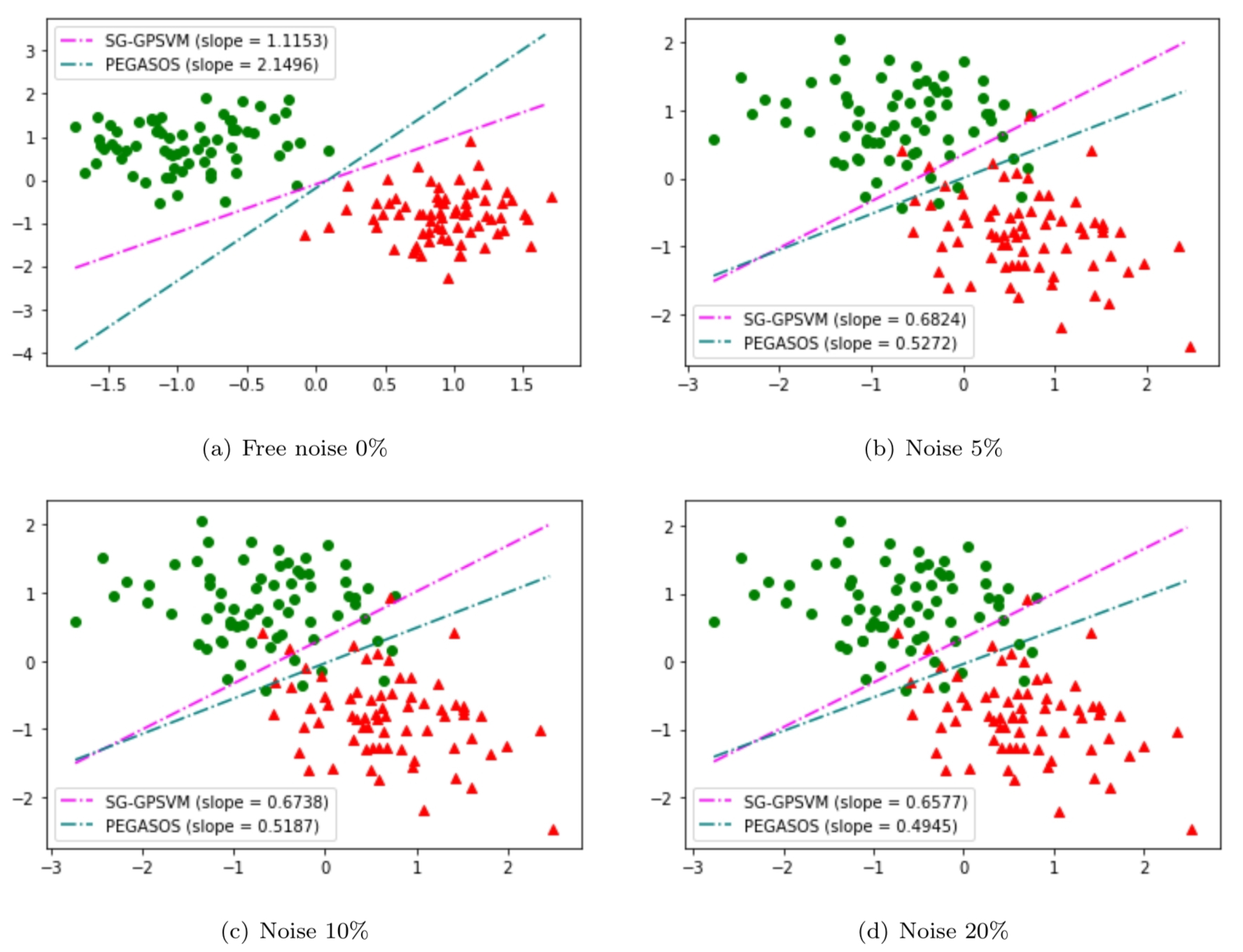
5.1. Artificial Datasets

We conducted experiments on a two-dimensional example, for which the samples came from two Gaussian distributions with equal probability: $x_i,i\in \{i:y_i=1\}\sim \mathcal{N}({\mu }_1,{\Sigma }_1)$ and $x_i,i\in \{i:y_i=-1\}\sim \mathcal{N}({\mu }_2,{\Sigma }_2)$ where ${\mu }_1={[1,-3]}^{\top },{\mu }_2={[-1,3]}^{\top }$ and ${\Sigma }_1={\Sigma }_2=\left[\begin{array}{cc}0.2& 0\\ 0& 3\end{array}\right]$. We added noise to the dataset. The labels of the noise points were selected from $\{1,-1\}$ with equal probabilities. Each noisy sample was drawn from a Gaussian distribution $\mathcal{N}({\mu }_n,{\Sigma }_n)$ where ${\mu }_n={[0,0]}^{\top }$ and ${\Sigma }_n=\left[\begin{array}{cc}1& -0.8\\ -0.8& 1\end{array}\right]$. This noise affects the labels around the boundary. The level of noise was controlled by the ratio of the noisy data in the training set, denoted by r. The value of r was fixed at $r=0$ (i.e., noise-free), $0.05,0.1$, and $0.2$. All the results of the two algorithms, SG-GPSVM and Pegasos, were derived using the two-dimensional dataset shown in Figure 1. Here, green circles denote samples from Class 1 and red triangles represent data samples from Class $-1$. From Figure 1, we can see that the noisy samples affect the labels around the decision boundary. As we increase the amount of noise from $r=0\%$ to $r=20\%$, the hyperplanes of Pegasos start deviating from the ideal slope of 2.14, whereas the deviation in the slopes of the hyperplanes is significantly less in our SG-GPSVM. This implies that our purposed algorithm is insensitive to noise around the decision boundary.

Figure 1. SG-GPSVM and Pegasos on a noisy artificial dataset. The above four figures demonstrate the noise-insensitive properties of our purposed SG-GPSVM compared to Pegasos when we have: (a) $r=0$ (noise free); (b) $r=0.05$; (c) $r=0.1$; (d) $r=0.2$.

5.2. UCI Datasets

We also performed experiments on 11 benchmark datasets available in the UCI Machine Learning Repository. Table 1 lists the datasets and their descriptions. For the benchmarks, we compared SG-GPSVM with two other SVM-based classical classifiers: conventional SVM and Pegasos. Among these SVM models, Pegasos and SG-GPSVM have extra hyperparameters, in addition to the hyperparameter C. The performance of different algorithms depends on the choices of the parameters [33,36,37]. All the hyperparameters were chosen through the grid search method and manual adjustment. The 10-fold cross-validation evaluation method was also employed. In each algorithm, the optimal parameter C was searched from set $\left\{{10}^i\right|i=-2,-1,0,1,2\}$, and other parameters were searched from set $\{0.1,0.25,0.5,0.75,1\}$. Further, the kernel method was adopted to evaluate the performance of SG-GPSVM as a nonlinear classifier, where the RBF kernel was adopted. The parameter of the RBF kernel is $\gamma$, searched from set $\left\{{10}^i\right|i=-2,-1,0,1,2\}$. The results of the numerical experiments are shown in Table 2, and the optimal parameters used in Table 2 are summarized in Table 3.

Table 1. Description of the UCI datasets.

Datasets	# of Samples	# of Features	# in Negative Class	# in Positive Class
Appendicitis	106	7	85	21
Ionosphere	351	33	126	225
Monk-2	432	6	204	228
Monk-3	432	6	204	228
Saheart	462	9	302	160
WDBC	569	30	357	212
Australian	690	14	383	307
Spambase	4597	57	2785	1812
Phoneme	5404	5	3818	1586
Twonorm	7400	21	3703	3697
Coil2000	9822	86	9236	586

Table 2. Accuracy obtained on the UCI datasets using the linear and nonlinear (${}^{*}$) kernel.

Datasets	r	SVM	Pegasos	SG-GPSVM	SG-GPSVM ${}^{*}$
		Time (s)	Time (s)	Time (s)	Time (s)
Appendicitis	0	85.82 ± 14.33	83.82 ± 13.72	84.82 ± 13.02	87.91 ± 10.45
		0.0008	0.3198	0.4800	0.0899
	0.05	83.00 ± 14.17	81.82 ± 15.16	84.73 ± 11.34	88.91 ± 10.74
		0.0020	0.3099	0.4321	0.0883
	0.10	84.00 ± 8.61	85.55 ± 14.96	85.64 ± 13.33	86.91 ± 9.69
		0.0020	0.3169	0.4393	0.0887
	0.20	80.18 ± 13.51	79.18 ± 12.74	84.82 ± 13.55	86.82 ± 12.38
		0.0015	0.2962	0.4972	0.0880
Phoneme	0	77.48 ± 1.41	75.98 ± 1.96	77.31 ± 1.40	77.15 ± 2.64
		0.5502	0.3102	0.4015	0.0893
	0.05	77.42 ± 1.44	77.15 ± 2.020	77.44 ± 1.56	76.87 ± 2.07
		0.5153	0.3490	0.4197	0.0891
	0.10	77.18 ± 1.58	76.59 ± 1.71	76.48 ± 1.81	76.61 ± 2.15
		0.5020	0.3087	0.4083	0.0891
	0.20	76.76 ± 1.69	75.61 ± 1.63	76.33 ± 1.57	76.44 ± 2.33
		0.5210	0.3016	0.3917	0.0893
Monk-2	0	80.32 ± 8.96	79.85 ± 8.12	80.80 ± 7.66	81.48 ± 7.54
		0.0134	0.2993	0.4268	0.0891
	0.05	80.55 ± 8.96	79.38 ± 7.93	79.16 ± 6.33	79.86 ± 7.98
		0.0027	0.2835	0.4038	0.0894
	0.10	79.39 ± 8.55	76.60 ± 6.33	80.54 ± 7.82	80.53 ± 6.56
		0.0023	0.2886	0.3876	0.0894
	0.20	79.40 ± 7.07	77.09 ± 7.56	80.32 ± 8.14	80.11 ± 5.54
		0.0025	0.3099	0.3815	0.0900
Monk-3	0	80.53 ± 4.61	77.75 ± 5.68	80.30 ± 4.50	84.47 ± 4.82
		0.0047	0.2835	0.4899	0.0947
	0.05	80.35 ± 4.75	78.01 ± 4.03	80.30 ± 4.38	84.23 ± 8.64
		0.0067	0.2932	0.4856	0.0970
	0.10	78.69 ± 3.46	79.40 ± 4.59	80.07 ± 4.50	83.31 ± 8.07
		0.0031	0.2974	0.4675	0.0956
	0.20	77.99 ± 4.86	77.32 ± 6.28	80.32 ± 3.36	81.93 ± 6.99
		0.0016	0.2875	0.4918	0.0994
Saheart	0	71.83 ± 7.22	70.52 ± 6.62	72.49 ± 7.45	72.32 ± 4.42
		0.0047	0.3071	0.4038	1.4542
	0.05	71.39 ± 7.66	71.84 ± 5.01	72.48 ± 6.70	71.87 ± 3.91
		0.0047	0.2989	0.3816	1.4453
	0.10	72.27 ± 7.11	67.98 ± 4.19	71.38 ± 8.65	71.00 ± 5.38
		0.0052	0.3249	0.4107	1.4201
	0.20	72.50 ± 7.65	72.47 ± 8.19	71.82 ± 10.10	70.80 ± 6.23
		0.0051	0.3160	0.3830	1.4503
Ionosphere	0	88.32 ± 6.94	84.02 ± 8.32	86.60 ± 6.15	91.46 ± 5.25
		0.0080	0.3541	0.3913	0.0944
	0.05	87.46 ± 5.75	86.03 ± 5.35	86.88 ± 6.30	91.45 ± 2.86
		0.0046	0.3176	0.4110	0.0937
	0.10	83.74 ± 7.15	84.60 ± 6.31	86.03 ± 7.83	91.17 ± 3.25
		0.0076	0.3160	0.8683	0.0941
	0.20	82.31 ± 7.78	85.46 ± 4.88	87.73 ± 5.74	90.03 ± 5.12
		0.0079	0.3233	0.4122	0.0936

Note: * Nonlinear case.

Table 3. The optimal parameters of conventional SVM, Pegasos, SG-GPSVM, and SG-GPSVM ${}^{*}$.

Datasets	SVM	Pegasos	SG-GPSVM	SG-GPSVM ${}^{*}$
	$\mathit{C}$	$\mathit{C}$	$\mathit{C},{\mathbf{\tau }}_{\mathbf{1}},{\mathbf{\tau }}_{\mathbf{2}},$ ${\mathbf{ϵ}}_{\mathbf{1}},{\mathbf{ϵ}}_{\mathbf{2}}$	$\mathit{C},{\mathbf{\tau }}_{\mathbf{1}},{\mathbf{\tau }}_{\mathbf{2}},$ ${\mathbf{ϵ}}_{\mathbf{1}},{\mathbf{ϵ}}_{\mathbf{2}}$,$\mathbf{\gamma }$
Appendicitis	1	10	100, 0.5, 0.75, 0.1, 1	10, 1, 1, 0.5, 0.5, 0.1
Phoneme	1	1	10, 0.5, 0.5, 0.1, 1	100, 1, 1, 0.25, 0.25, 1
Monk-2	1	0.01	100, 1, 0.25, 0.1, 0.25	100, 0.25, 0.25, 0.1, 0.25, 0.1
Monk-3	1	0.1	1, 1, 0.25, 0.5, 0.5	10, 1, 0.75, 0.25, 0.25, 0.1
Saheart	1	1	1, 0.5, 0.25, 0.25, 0.1	100, 1, 0.75, 0.25, 0.25, 0.1
Ionosphere	1	1	1, 0.75, 0.1, 0.25, 0.1	100, 1, 1, 1, 0.5, 0.1

Note: * Nonlinear case.

Table 2 shows the results for a linear and nonlinear kernel on six different UCI datasets by applying conventional SVM, Pegasos, and our proposed SG-GPSVM. From the experimental outcomes, it can be seen that the classification performance of SG-GPSVM is better than that of the conventional SVM and Pegasos on most of the datasets in terms of accuracy. From Table 2, our proposed SG-GPSVM yielded the best prediction accuracy on four of six datasets. In addition, when we varied the number of noisy samples from $r=0$ (noise-free) to $r=0.2$, our proposed SG-GPSVM exhibited better classification accuracy and stability than the other algorithms no matter the noise factor value, as shown in Figure 2. On the Appendicitis dataset, when the noise factor increased, the accuracy of the conventional SVM and Pegasos fluctuated greatly. On the contrary, the classification accuracies of our proposed SG-GPSVM were stable. Similarly, on the other datasets, such as Monk-3 and Appendicitis, the accuracies of the conventional SVM and Pegasos not only varied greatly, but they also performed worse than our proposed algorithm. This demonstrates that our proposed SG-GPSVM is relatively stable, regardless of the noise factor. In terms of computational time, our proposed algorithm cost nearly the same as Pegasos. The computational time of Pegasos and our proposed SG-GPSVM on the largest dataset was longer than the computational time of the conventional SVM on the smaller datasets.

Figure 2. The accuracy of four algorithms with different noise factors on six datasets: (a) Appendicitis; (b) Ionosphere; (c) Monk-2; (d) Monk-3; (e) Phoneme; (f) Saheart.

The experimental results of three different minibatches for SG-GPSVM $(1,32,512)$ and the accuracy and computational time results of the methods are illustrated in Figure 3. Subfigure (a) shows how the accuracy changed in terms of the batch size, and the curves in Subfigure (b) show how the computational time changed in terms of the batch size. We can see that when the size of the minibatch increased, the accuracy increased, and the computational time increased approximately linearly when the batch size increased. The datasets Spambase and WDBC were taken into consideration. It is evident that if the minibatch size k is small enough, $k=32$ is more accurate than $k=512$. However, when using a large minibatch size of $k=512$, the accuracy decreased and the computational time increased. This suggests that in the scenarios in which we care more about the accuracy, we should choose a relatively medium batch size (it does not need to be large).

Figure 3. Classification results on the UCI datasets with minibatch SG-GPSVM. (a) Accuracy of minibatch SG-GPSVM. (b) Computational time of minibatch SG-GPSVM.

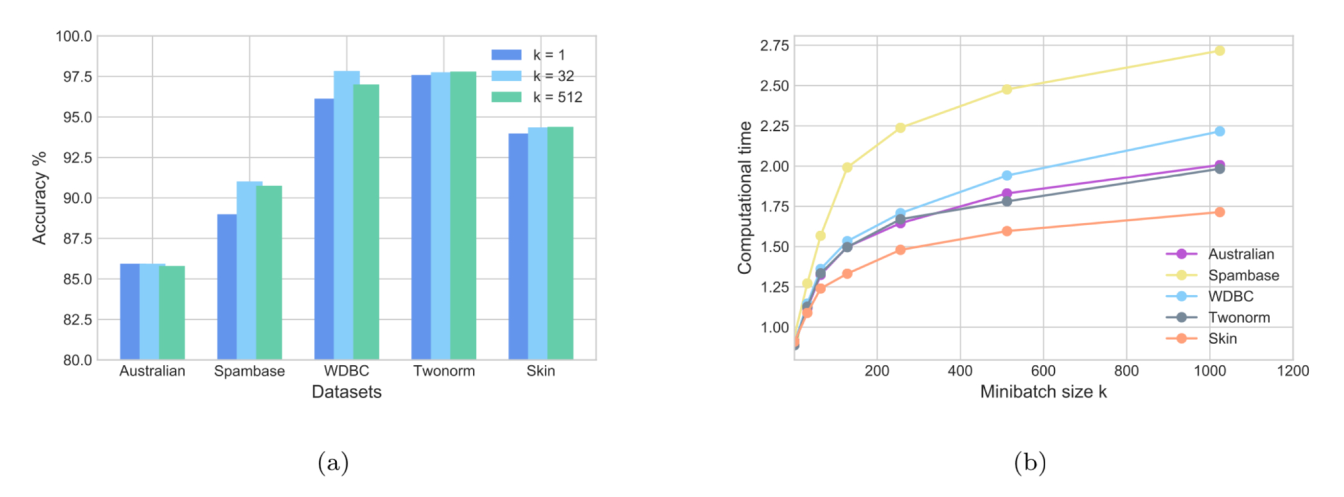
5.3. Large-Scale Dataset

In order to validate the classification efficiency of SG-GPSVM, we conducted comparisons of our methods with the two most related methods (SVM and Pegasos) on four large-scale UCI datasets. We show that our SG-GPSVM is capable of solving large-scale problems. Note that the results of this section were solved on a machine equipped with an Intel CPU E5-2658 v3 at 2.20 GHz and 256 GB RAM running the Ubuntu Linux operating system. The scikit-learn package was sued for the conventional SVM [35]. The large-scale datasets are presented in Table 4.

Table 4. The details of the large-scale datasets.

Datasets	# of Samples	# of Features	# in Negative Class	# in Positive Class
Credit card	30,000	324	23,364	6636
Skin	245,057	3	194,198	50,859
Kddcup	4,898,431	41	972,781	3,925,650
SUSY	5,000,000	18	2,712,173	2,287,827

For the four large-scale datasets, we compare the performance of SG-GPSVM against the conventional SVM and Pegasos in Table 5. The reduced kernel [38] was employed in the nonlinear situation, and the kernel size was set to 100. From the results in Table 5, SG-GPSVM outperformed the conventional SVM and Pegasos on three out of the four datasets in terms of accuracy. The best ones are highlighted in bold. However, SG-GPSVM’s accuracy on some datasets, such as Credit card, was not the best. On the Skin dataset, the conventional SVM performed much worse than SG-GPSVM and Pegasos, and it was not possible to use the conventional SVM on the Kddcup and Susy datasets due to the high memory requirements. This was because SVM requires the complete training set to be stored in the main memory. On the Credit card dataset, our proposed SG-GPSVM took almost the same amount of time as the conventional SVM and Pegasos. Our suggested approach, SG-GPSVM, took almost the same amount of time as Pegasos on the Kddcup and Susy datasets.

Table 5. Classification results on the large-scale UCI datasets.

Datasets	Mean Accuracy in %
	Credit Card	Skin	Kddcup	Susy
SVM	80.82 ± 0.90	92.90 ± 0.16	*	*
Time (s)	0.4398	289.4454	*	*
Pegasos	79.74 ± 2.38	93.22 ± 0.78	95.31 ± 0.31	99.25 ± 1.37
Time (s)	0.2479	0.2676	1.9823	4.5164
SG-GPSVM	80.72 ± 0.95	93.98 ± 0.38	98.82 ± 0.60	99.97 ± 0.06
Time (s)	0.4417	0.3751	2.0474	5.3744
SG-GPSVM ${}^{*}$	77.88 ± 0.87	94.06 ± 1.13	96.92 ± 0.35	99.99 ± 0.02
Time (s)	1.0881	0.9738	2.8125	2.3218

Note: * Nonlinear case.

6. Conclusions

In this paper, we used the generalized pinball loss function in SVM to perform classification and proposed the SG-GPSVM classifier. This paper adapted the stochastic subgradient descent method as stochastic subgradient descent method-based generalized pinball SVM (SG-GPSVM). Compared to the hinge loss SVM and Pegasos, the major advantage of our proposed method is that SG-GPSVM is less sensitive to noise, especially the feature noise around the decision boundary. In addition, we investigated the convergence of SG-GPSVM and the theoretical approximation between GPSVM and SG-GPSVM. The validity of our proposed SG-GPSVM was demonstrated by numerical experiments on artificial datasets and datasets from UCI with noises of different variances. The experimental results clearly showed that our suggested SG-GPSVM outperformed the existing classifier approach in terms of accuracy, and SG-GPSVM has a significant advantage in handling large-scale classification problems. The results imply that the SG-GPSVM approach is the strongest candidate for solving binary classification problems.

In further work, we would like to consider applications of SG-GPSVM to activity recognition datasets and image retrieval datasets, and we also plan to improve our approach to deal with multicategory classification scenarios.

References

1. Vapnik, V.N. The Nature of Statistical Learning Theory; Springer: New York, NY, USA, 1995. [Google Scholar]
2. Vapnik, V.N. Statistical Learning Theory; Wiley: New York, NY, USA, 1998. [Google Scholar]
3. Vapnik, V.N. An overview of statistical learning theory. IEEE Trans. Neural Netw. 1999, 10, 988–999. [Google Scholar] [CrossRef] [PubMed] [Green Version]
4. Colmenarez, A.J.; Huang, T.S. Face Detection With Information-Based Maximum Discrimination. In Proceedings of the IEEE Computer Society Conference on Computer Vision and Pattern Recognition, San Juan, PR, USA, 17–19 June 1997; pp. 782–787. [Google Scholar]
5. Osuna, E.; Freund, R.; Girosi, F. Training support vector machines: An application to face detection. In Proceedings of the IEEE Computer Vision and Pattern Recognition, San Juan, PR, USA, 17–19 June 1997. [Google Scholar]
6. Joachims, T.; Ndellec, C.; Rouveriol, C. Text categorization with support vector machines: Learning with many relevant features. In Proceedings of the European Conference on Machine Learning, Chemnitz, Germany, 21–23 April 1998; pp. 137–142. [Google Scholar]
7. Richhariya, B.; Tanveer, M. EEG signal classification using universum support vector machine. Expert Syst. Appl. 2018, 106, 169–182. [Google Scholar] [CrossRef]
8. Mukherjee, S.; Osuna, E.; Girosi, F. Nonliner prediction of chaotic time series using a support vector machine. In Proceedings of the 1997 IEEE Workshop on Neural Networks for Signal Processing, Amelia Island, FL, USA, 24–26 September 1997. [Google Scholar]
9. Ince, H.; Trafalis, T.B. Support vector machine for regression and applications to financial forecasting. In Proceedings of the International Joint Conference on Neural Networks (IEEE-INNSENNS), Como, Italy, 27 July 2000. [Google Scholar]
10. Huang, Z.; Chen, H.; Hsua, C.-J.; Chen, W.-H.; Wu, S. Credit rating analysis with support vector machines and neural networks: A market comparative study. Decis. Support Syst. 2004, 37, 543–558. [Google Scholar] [CrossRef]
11. Khemchandani, R.; Jayadeva; Chandra, S. Regularized least squares fuzzy support vector regression for nancial time series forecasting. Expert Syst. Appl. 2009, 36, 132–138. [Google Scholar] [CrossRef]
12. Tao, D.; Tang, X.; Li, X.; Wu, X. Asymmetric bagging and random subspace for support vector machines-based relevance feedback in image retrieval. IEEE Trans. Pattern Anal. Mach. Intell. 2008, 28, 1088–1099. [Google Scholar]
13. Pal, M.; Mather, P. Support vector machines for classification in remote sensing. Int. J. Remote Sens. 2005, 26, 1007–1011. [Google Scholar] [CrossRef]
14. Li, Y.Q.; Guan, C.T. Joint feature re-extraction and classification using an iterative semi-supervised support vector machine algorithm. Mach. Learn. 2008, 71, 33–53. [Google Scholar] [CrossRef]
15. Bi, J.; Zhang, T. Support vector classification with input data uncertainty. In Proceedings of the Neural Information Processing Systems, Vancouver, BC, Canada, 13–18 December 2004. [Google Scholar]
16. Huang, X.; Shi, L.; Suykens, J.A.K. Support vector machine classifier with pinball loss. IEEE Trans. Pattern Anal. Mach. Intell. 2014, 36, 984–997. [Google Scholar] [CrossRef]
17. Rastogi, R.; Pal, A.; Chandra, S. Generalized pinball loss SVMs. Neurocomputing 2018, 322, 151–165. [Google Scholar] [CrossRef]
18. Ñanculef, R.; Frandi, E.; Sartori, C.; Allende, H. A Novel Frank-Wolfe Algorithm. Analysis and Applications to Large-Scale SVM Training. Inf. Sci. 2014, 285, 66–99. [Google Scholar] [CrossRef] [Green Version]
19. Xu, J.; Xu, C.; Zou, B.; Tang, Y.Y.; Peng, J.; You, X. New incremental learning algorithm with support vector machines. IEEE Trans. Syst. Man Cybern. Syst. 2018, 49, 2230–2241. [Google Scholar] [CrossRef]
20. Platt, J. Fast training of support vector machines using sequential minimal optimization. In Advances in Kernel Methods—Support Vector Learning; MIT Press: Cambridge, MA, USA, 1999; pp. 185–208. [Google Scholar]
21. Mangasarian, O.; Musicant, D. Successive overrelaxation for support vector machines. IEEE Trans. Neural Netw. 1999, 10, 1032–1037. [Google Scholar] [CrossRef] [Green Version]
22. Fan, R.; Chang, K.; Hsieh, C.; Wang, X.; Lin, C. LIBLINEAR: A library for large linear classification. J. Mach. Learn. Res. 2008, 9, 1871–1874. [Google Scholar]
23. Zhang, T. Solving large-scale linear prediction problems using stochastic gradient descent algorithms. In Proceedings of the International Conference on Machine Learning, Banff, AB, Canada, 4–8 July 2004. [Google Scholar]
24. Xu, W. Towards optimal one pass large-scale learning with averaged stochastic gradient descent. arXiv 2011, arXiv:1107.2490. [Google Scholar]
25. Shai, S.; Singer, Y.; Srebro, N.; Cotter, A. Pegasos: Primal estimated subgradient solver for SVM. Math. Program. 2011, 127, 3–30. [Google Scholar]
26. Alencar, M.; Oliveira, D.J. Online learning early skip decision method for the hevc inter process using the SVM-based Pegasos algorithm. Electron. Lett. 2016, 52, 1227–1229. [Google Scholar]
27. Reyes-Ortiz, J.; Oneto, L.; Anguita, D. Big data analytics in the cloud: Spark on Hadoop vs MPI/OpenMP on Beowulf. Procedia Comput. Sci. 2015, 53, 121–130. [Google Scholar] [CrossRef] [Green Version]
28. Sopyla, K.; Drozda, P. Stochastic gradient descent with barzilaicborwein update step for SVM. Inf. Sci. 2015, 316, 218–233. [Google Scholar] [CrossRef]
29. Dua, D.; Taniskidou, E.K. UCI Machine Learning Repository; School of Information and Computer Science, University of California: Irvine, CA, USA, 2019; Available online: http://archive.ics.uci.edu/ml (accessed on 24 September 2018).
30. Shwartz, S.; Ben-David, S. Understanding Machine Learning Theory Algorithms; Cambridge University Press: Cambridge, MA, USA, 2014; 207p. [Google Scholar]
31. Xu, Y.; Yang, Z.; Pan, X. A novel twin support-vector machine with pinball loss. IEEE Trans. Neural Netw. Learn. Syst. 2017, 28, 359–370. [Google Scholar] [CrossRef]
32. Shao, Y.; Zhang, C.; Wang, X.; Deng, N. Improvements on twin support vector machines. IEEE Trans. Neural Netw. 2011, 22, 962–968. [Google Scholar] [CrossRef] [PubMed]
33. Khemchandani, R.; Jayadeva; Chandra, S. Optimal kernel selection in twin support vector machines. Optim. Lett. 2009, 3, 77–88. [Google Scholar] [CrossRef]
34. Rudin, W. Principles of Mathematical Analysis, 3rd ed.; McGraw-Hill: New York, NY, USA, 1964. [Google Scholar]
35. Pedregosa, F.; Varoquaux, G.; Gramfort, A.; Michel, V.; Thirion, B.; Grisel, O.; Blondel, M.; Prettenhofer, P.; Weiss, R.; Dubourg, V.; et al. Scikit-learn: Machine learning in Python. J. Mach. Learn. Res. 2011, 12, 2825–2830. [Google Scholar]
36. Cristianini, N.; Shawe-Taylor, J. An Introduction to Support Vector Machines and Other Kernel-Based Learning Methods; Cambridge University Press: Cambridge, UK, 2000. [Google Scholar]
37. Shawe-Taylor, J.; Cristianini, N. Kernel Methods for Pattern Analysis; Cambridge University Press: Cambridge, UK, 2004. [Google Scholar]
38. Lee, Y.; Mangasarian, O. RSVM: Reduced support vector machines. In Proceedings of the First SIAM International Conference on Data Mining, Chicago, IL, USA, 5–7 April 2001. [Google Scholar]
Publisher’s Note: MDPI stays neutral with regard to jurisdictional claims in published maps and institutional affiliations.
Article Metrics
Citations
Article Access Statistics
Multiple requests from the same IP address are counted as one view.