A Weight Assignment Algorithm for Incomplete Traffic Information Road Based on Fuzzy Random Forest Method

Abstract

One of the keys in time-dependent routing is determining the weight for each road network link based on symmetrical and complete traffic information. To facilitate travel planning considering traffic situations based on historical global position system (GPS) trajectory data which uncover the whole road network, this paper proposes a fuzzy random forest-based road section data estimation method, which uses the third law of geography as the core idea. For different time periods, road grade, tidal lane, proximity to infrastructure (main places that affect traffic, such as schools, hospitals), and accident road sections were selected as indicators that influence the traffic. The random forest algorithm is used to build the mapping relationship between attribute data with average traffic which is obtained based on GPS data. Subsequently, the fuzzy reasoning method is used to obtain the weight of road links missing traffic information by calculating their similarities with typical road section samples. Using the road network of Suzhou City as an example, the proposed method was used to analyze estimate the average driving speeds of road sections with missing traffic information for different time periods. Experimental results show that this method can effectively avoid congested road sections and obtain high-speed travel routes.

1. Introduction

Traffic congestion has become a major problem in cities as the number of vehicles on city roads has increased. Waiting in traffic wastes time and has an adverse economic impact. To minimize the costs incurred by waiting in traffic, people can plan their routes with the shortest travel time. Towards this end, the road weights containing traffic information can be used in a route optimization algorithm. The weight value determines the search basis of the common path algorithms and affects the rationality of the optimal path. However, the traffic data in many cities cannot cover the whole road network yet. In most cities, the traffic information is collected by sensors or Taxi GPS trajectory data, the sensors are usually installed at the main roads and there are still a lot of roads lacking traffic data records, Taxi GPS trajectory data also cannot cover the whole road. This means that in the case of data missing, the weight of the whole road links cannot be generated.

The lack of traffic data on some road sections has two primary types: the partial or complete lack of road traffic data. A partial lack of road traffic data means that the road section lacks traffic data for a given date-time range and it can be inferred from the data of other dates at that time, or from historical data. A complete lack of road traffic data means that the road section has no GPS data at all. This situation requires that the missing data be filled out by data from other roads in the road network.

In the face of a partial lack of road traffic data, the weight of road network can be determined by using real-time traffic data and historical traffic data. The two commonly used methods of weight calculation are: using up-to-date traffic information to calculate the current weight, and using historical traffic information to predict the weight. For the first method, impedance function models are usually used to determine the time cost of each road link. Examples of such models are the Bureau of Public Roads (BPR) model [1,2], the Davidson model [3,4,5,6,7], and the multiclass user traffic equilibrium model [6,7]. Additionally, the traffic flow fluctuation theory can be applied to determine the travel time of the road section with missing traffic data by obtaining the travel time of the known road section and establishing a dynamic allocation recursive function [8,9,10,11].

For the second method, the basic idea is to ascertain the traffic rules based on basic historical information and to use current information to predict real-time weights. Along this line of reasoning, Zhu et al. proposed a two-stage routing algorithm and weight propagation model to predict the cost of an arbitrary path on a road network and accurately detect the traffic environment [12]. Tang proposed a road network path-planning algorithm based on experience levels. By analyzing historical floating car data (FCD) to determine the experience level of road sections, significantly faster path planning results can be obtained [13,14,15].

2. Related Works

To deal with the complete lack of traffic data for road sections, some researchers generate the weight of the entire road section from incomplete road section information. Yang’s study was the first to completely annotate the weights of road networks using incomplete information. Yang used regression to model the problem and took the topology of the road network into account to construct the objective function. This method attempts to find a road section with the most similar and closest distance to the road section with missing traffic information from the road sections with complete traffic data, and sets the distribution and quantity of traffic flow and infrastructure as the influence index of the predicted vehicle speed, and uses the linear method to determine road weight. Yang’s approach is a good reference for the calculation of the road links’ weights with incomplete information [16]. Similarly, Zambrano-Martinez applied logistic regression and proposed an equation, being able to significantly improve the curve fitting results [17]. In fact, the vehicle speed is not only impacted by traffic flow but also impacted by other factors which are not linear, it cannot reflect these complex impacts just uses a regression model to describe it.

On this basis, more complex models are proposed. Ashok presented a model for the estimation and prediction of time-dependent origin–destination (O-D) matrices, it estimated the dynamic mapping between the time-dependent O-D flow and the link volume [18]. The O-D model can be divided into two categories: direct estimation and model estimation [19]. The direct estimation method uses the expanded sampling survey, which costs a lot of time. The model estimation method uses the traffic flow to establish the travel demand model and get the predicted O-D flow. Nguyen, T.V. et al. proposed the open source DFROUTER tool. It could obtain the O-D matrix that represents the internal trips inside the target area, and it resembled the real traffic distribution in the city [20]. The O-D model is easy to be applied in small networks, but a large number of road traffic data need to be input to improve the accuracy [21]. Shang et al. constructing a space–time–state hyper network by using a triple of flow, density and speed, it estimates the level of traffic congestion and provides decisions for traffic planning [22]. The influence of various activity attributes on the spatial and temporal distribution of road traffic flow is considered. However, when the network scale is large, it is necessary to enumerate all the possible states of nodes, so the calculation cost is high. Charbonneau proposed a heuristic algorithm, the shortest path heuristic algorithm (SPT). SPT uses the minimum path heuristic to create a Steiner tree to destination, it essentially considers the closest nodes instead of all possible node. On the basis of a current solution, it optimizes step by step through neighborhood search [23]. SPT method is not easy to fall into local optimum, but the algorithm is very complex, many parameters are considered, and the efficiency is not high [24]. The above methods are only suitable for small traffic networks, and need to be improved when there are more nodes. Zambrano-Martinez et al. proposed a route server capable of handling all the traffic in a city, and balancing traffic flows by accounting for present and future traffic congestion conditions. With the increasing popularity of autonomous vehicles, congestion problems might be more common shortly. The focus on autonomous vehicles also allowed for more predictive behavior on the road. It showed that their model improved travel times and average travel speed in Valencia, Spain by 5%. In more congested areas, this improvement was about 8% [25]. Quiroga proposed a localization system to estimate traffic conditions [26], using the precise information provided by GPS, the real-time traffic information of each section of the city is obtained through mathematical modeling, and the current traffic flow or congestion situation is judged. It analyzed the sampled GPS data by segment lengths, sampling rates, and central tendency [27]. Then the average speed, traffic flow and other information of the path are calculated according to the GPS data and mathematical model, and then the traffic situation is estimated. This method is difficult to acquire complete and symmetrical GPS data through automatic acquisition, however, if the manual acquisition method is used, it will require a lot of work.

The above analysis showed that, given the complete lack of traffic data on road sections, traditional methods were suitable for small networks and were complicated. Although the new methods based on machine learning and metaheuristic techniques have improved, they could predict long-term traffic speed [28]. The method based on machine learning is fast to calculate, and it does not need a lot of input variables. However, the single machine learning method was difficult to accurately generate the impedance for incomplete information road links. These problems could be avoided. It was necessary to find the main factors affecting traffic and the similarity with different typical road sections. These were rarely considered in the existing methods. The key point was finding the data which were related to these traffic impact factors. A representative number of typical road sections could be extracted from road links as a template through expert knowledge, and we called this template a typical link pattern (TLP). These TLPs had complete information, which meant that both average speeds and the factors impacting on traffic of these road links were known. If we set various factors values to TLPs and calculated the similarity between incomplete information road link and the TLPs, the TLP which had the maximum similarity with this road link could be used to calculate weight further.

This paper differs from previous works by combining machine learning with fuzzy rules. Looking at actual situations where historical GPS data cannot cover the entire road network and there are no traffic data for some road sections [29], this paper proposes a road impedance estimation model based on fuzzy random forest, which considers the third law of geography as its guiding principle. The third law of geography says that the greater the similarities between geographical environments, the more similar the characteristics of the geographical target. Geographical similarity referred to the comprehensive similarity of two spatial locations in the geographic environment, and these two locations are not necessarily connected in space. Geographical features referred to the characteristics of the geographical variables concerned [30]. In other words, if the factors affecting traffic at specific times are similar, vehicle speeds should also be similar. In our study, the road level, driving speed, whether there are important traffic units around, whether the road is a tidal lane, whether it is an accident section, and road sampling time are all factors that affect traffic. Firstly, the random forest is used to establish the complete information road section, that is, the mapping relationship between the traffic factors and the incomplete information road section is established, and then the incomplete traffic information road section is input. Thereby, the impedance value of both complete information and incomplete road sections can be estimated.

3. Study Area and Data

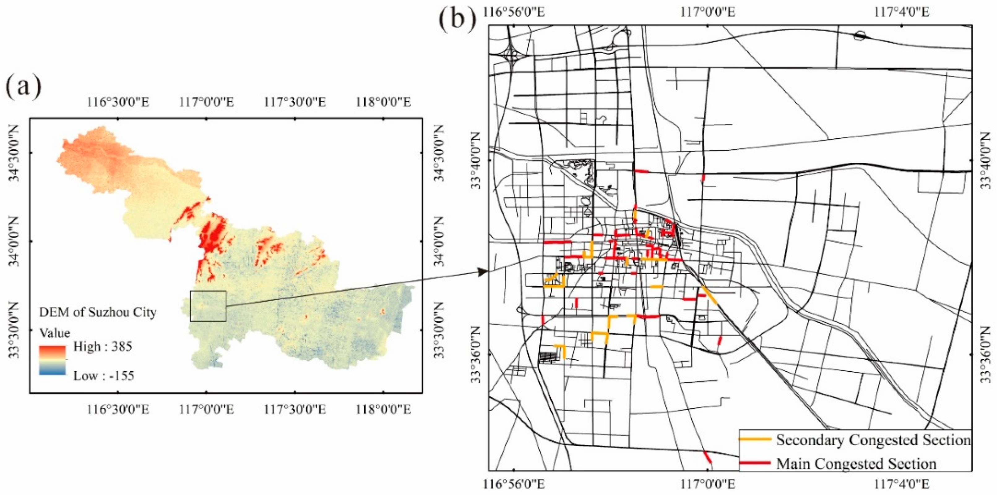
The area this paper chose to study is Suzhou City, Anhui Province, China (Figure 1a). Suzhou City is located north of Anhui Province and is a municipal district of Yongqiao district (Figure 1b). It is located between 116°09′ E–118°10′ E and 33°18′ N–34°38′ N. Yongqiao District is located at the junction of the provinces of Jiangsu, Henan, and Anhui. It is very convenient to get around in the city. The transportation network in Suzhou City has obvious temporal and spatial characteristics. Traffic congestion is pronounced during the morning and evening rush hours. The figure shows the road sections prone to congestion. The terrain of the study area is flat, with small undulation, various road types, and high-frequency GPS data (1–3 s) can be obtained, so it is an ideal area for the study.

In the study, we used taxi (114 vehicles) GPS data from Suzhou Traffic Management Bureau (http://jtj.ahsz.gov.cn/, accessed on 22 December 2019), which has a high frequency (1–3 s). We used taxi GPS data from January to March 2014, which covered 24 h a day, including time, longitude, latitude, speed and elevation. Among them, the speed is calculated by the distance and time between two points of GPS.

Table 1. High frequency GPS data and fields.

INDEX	DATA	TIME	LATITUDE	LONGITUDE	HEIGHT	SPEED
1	140115	11622	33.619021N	116.982741E	9	0
2	140115	11625	33.618906N	116.982789E	9	3
...	...	...	...	...	...	...

shows the GPS data, as imported into ArcGIS, and with calculations of the average speed of GPS points on the road in a specific period of time, that is, the average speed of this section in that period of time. “DATA 140114” represents 14 January 2014, “TIME 11622” represents 1:16:22 of the day.

4. Methodology

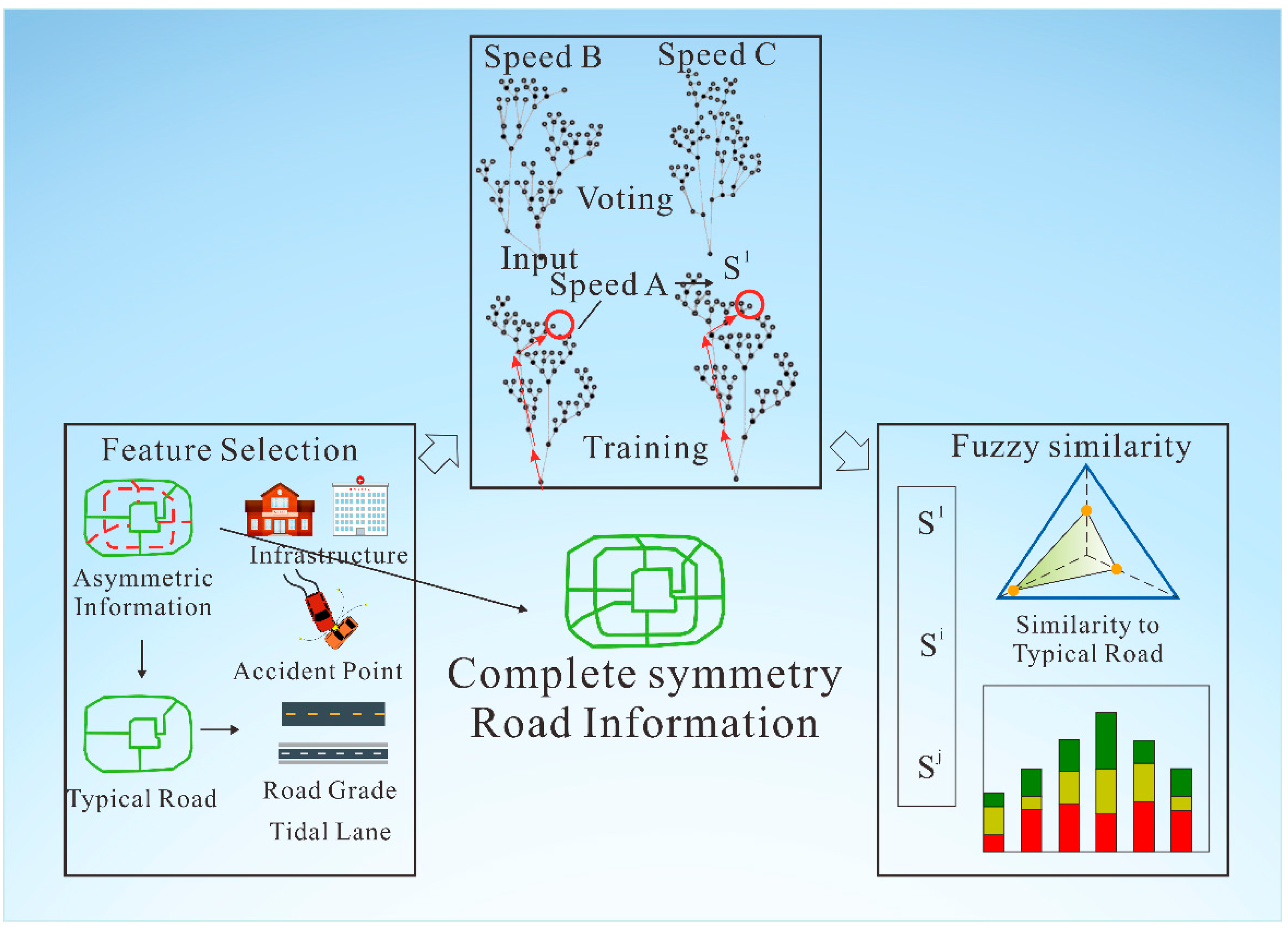
Due to the lack and asymmetry of road information, this paper brings out a new model to estimate the impedance of paths based on a random forest method. This model is based on the third law of geography, and it assumes that if the factors impact on the traffic are similar at a specified time, the vehicles speed is also similar, so the average speed of incomplete information road links can be evaluated by the full information road links through the fuzzy random forest and the average speed is the key for time-dependent routing calculating. The basic idea of this method is to first analyze the traffic influencing factors, extract typical road sections as training data, calculate the average speed of incomplete traffic information road sections through the fuzzy random forest, and then estimate the impedance value. Finally, the road network with complete and symmetrical information is generated, as shown in the conceptual illustration of fuzzy random forest (Figure 2).

The traffic condition of urban roads is produced by the combination of internal factors such as road grade and number of lanes and external factors. In the absence of traffic data, the road’s speed limit is typically used as the road’s weight. Since the road’s speed limit is usually faster than actual traffic speeds and these road sections are used in route planning, actual travel times tend to be longer than predicted ones. Therefore, the weights of road networks used in route planning must conform to the actual traffic conditions. As an intermediate parameter, the average driving speed establishes the relationship between distance and time in path planning. In this paper, the vehicle’s speed is directly related to the vehicle’s travel time and many other environmental factors affecting the road network. In other words, travel time is impacted by increases or decreases in speed. Environmental factors include road locality (e.g., a vehicle’s speed should be reduced when traveling on roads near schools and hospitals) and traffic conditions (e.g., average vehicles’ speeds will be very low on extremely congested road sections, like those found during the morning rush hours). In path optimization, roads with poor road conditions should have increased road impedance so that path planning is less likely to use that road. Therefore, setting the weight index to the speed of the vehicle reflects the time cost of driving on that road and establishes a connection with the distance or time weight. Establishing that connection is convenient for comparing path planning results. The basic idea of the fuzzy random forest method is to analyze traffic influencing factors, extract typical road sections, estimate the average speed of the road section, calculate the fuzzy similarity between average speeds and a typical road section that has complete information, and estimate the impedance value.

4.1. Road Network Weight Analysis

Many of Suzhou City’s roads have different features. There are two main factors affecting road traffic: the characteristics of the road itself (e.g., road grade, road length, road gradient, the number of lanes, etc.) and external factors (e.g., traffic volume, tidal effect, road locality, the number of traffic lights, traffic accidents, weather, etc.).

(1) Road grade

For the characteristics of the road itself, the road grade determines the material, flatness, design capacity, road width and other characteristics of the road. This paper’s expert knowledge of the characteristics of urban roads comes from the implementation of the “urban road engineering design specifications”.

Table 2. Speed limits for China’s roads.

Grade	Primary Road	Secondary Road	Third Level Road	Residential Road
Speed limit (km/h)	80	60	40	20
	70	50	30	10
	60	40	20	5

shows the speed limits for different road grades, and each grade includes three roads with different number of lanes, which have different speed limits. Therefore, when road information does not cover a road section, the road grade plays a decisive role in determining the average speed of that road section. Therefore, it is an important factor in estimating the impedance of road sections with incomplete traffic information. In the case where traffic information is unavailable, this study selects the vehicle speed observed during off-peak hours as the maximum road limit speed. The impact of weather on traffic is related to the city’s DEM (digital terrain model). Certain weather conditions (e.g., heavy rain and snowstorms) significantly impact average speeds. This paper does not consider the impact of road slopes because of the flatness of Suzhou City’s terrain.

(2) Tidal lane

Tidal effect means that the average speed of roads of the same grade is completely different in different time periods. The tidal effect is an important external factor that affects average vehicle speeds. Additionally, average vehicle speeds on the same road grade vary over time. We analyzed the spatial-temporal characteristics of traffic using Suzhou City’s historical traffic data. The traffic conditions throughout the day can be separated into four time periods. These periods are as follows: morning peak hour (7:00–9:00), evening peak hour (17:00–19:30), daytime hours (9:00–17:00) and night time (20:00–7:00 of the next day). Traffic flow is the main external factor that affects the speed of traffic, and there is a clear correlation between the two. Because it is difficult to obtain traffic flow data covering the entire road network, this paper used the average driving speeds for each road section during different times, as calculated from GPS historical data. The tidal effect has an evident regularity. This attribute can be directly assigned to the tidal road section, and the traffic condition of the road section can be determined according to the morning and evening peak times.

(3) Infrastructure and Accident point

Road section locality (whether near schools, hospitals, etc.) and whether the road section is an accident section are also main factors affecting traffic. Based on the third law of geography, we assumed that when the conditions of adjacent traffic units are similar at a given moment, their vehicle speeds are similar too. However, this effect is not linear. We analyzed traffic data from roads that are close to schools and hospitals, and accidental sections at various distances (less than 30 m, between 30–60 m, 60–100 m, and greater than 100 m). The results show that there is a significant difference between average road speeds of adjacent infrastructure (i.e., roads close to schools, hospitals, etc.)

The impact of weather on traffic is usually related to the DEM of a city. For example, heavy rain will have a significant impact on traffic in low-lying sections of the city, while heavy snow will have a greater impact on the traffic on slopes (e.g., bridge sections). Because of the flat terrain of this study’s research area, the impact of weather on road traffic in different sections of the city is neutralized. This is reflected in the average road speeds.

4.2. Road Network Weight Assignment Method Based on Fuzzy Random Forest

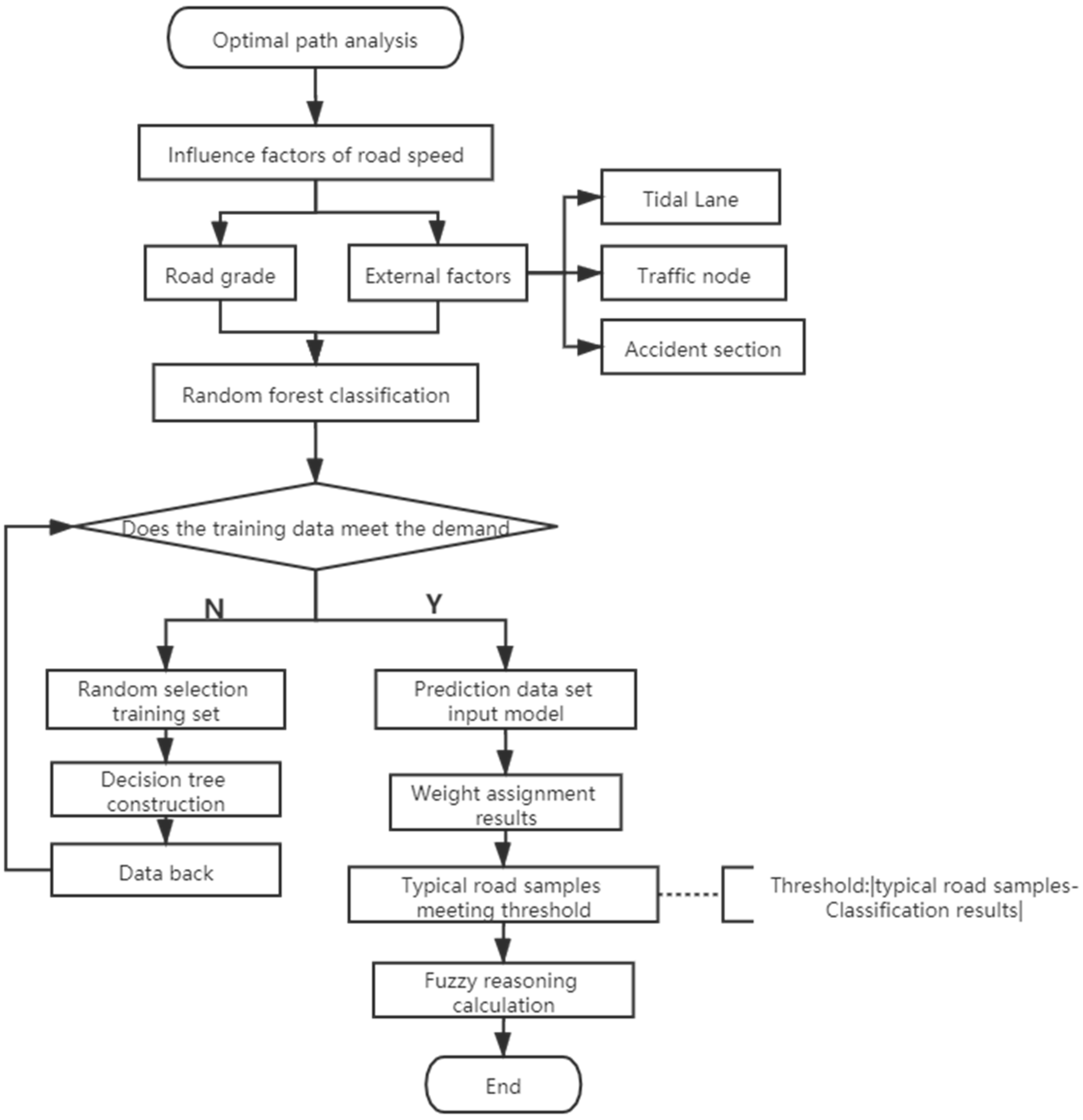
The amount of road network data is large, but the data coverage for some sections of the road network is lacking. It is difficult to calculate the average speed of all roads. Since travel time is affected by environmental factors, it is also difficult to directly construct a functional relationship between the impact factor and driving speeds. Therefore, we calculated the average road speeds for typical road sections in the road network using taxi GPS data, correlated with the environmental factors affecting a typical road section. This process is a typical road section sampling process. For road sections with missing data, the random forest classification method was used to obtain the average speed. In this way, the basic idea of road network weight assignment can be expressed as follows: take speed as the intermediate parameter of the road network weight, construct a mapping model between road network speeds and road environment factors, and collect data on the driving speed of typical road sections in the road network sampling using a random forest algorithm for classification mapping model training. The driving speed of other unsampled road sections can be determined according to the value of the environmental factor of the road section and the environmental factor of a typical road section. To assign a driving speed to an unsampled road section more accurately, this paper used fuzzy inference based on the random forest classification model. In this method, the similarity of environmental factors is used as the fuzzy membership degree to calculate the driving speed of the unsampled road section. Once the driving speed of the entire road network has been obtained, and the road weight matrix is constructed using that speed, and optimal path analysis is performed. The specific implementation steps are (Figure 3):

(1) Classified sampling

First, the characteristics of the road (e.g., road grade) and the external factors affecting traffic conditions (e.g., tidal lane, distance to traffic units, and accident sections) were selected according to the actual road conditions in the study area and the influencing factors of lane speeds. Second, with those characteristics, taxi GPS data were obtained to calculate the average vehicle speed of the corresponding road. Third, select typical road sections as samples to obtain the road speed value and its corresponding impact factors.

(2) Random forest classification

The road grade, tidal lane, distance to transportation units, and accident road sections were the independent variables of the training samples. Speed was the dependent variable. The random forest method was used to classify the training samples.

As a supervised learning algorithm, the random forest method selects training data and constructs a classifier in a random and replacement manner, and combines multiple models to form the final overall model. In contrast to the optimal threshold classification approach used by typical decision trees, the random forest classification process uses decision trees to classify data in a random threshold manner. This classification method can produce stronger diversity, improving the model’s results. The model construction and sample prediction process of the random forest method are as follows.

• From the original training dataset, randomly extract samples (approximately 30% of the dataset) to be the training set for a decision tree. This is repeated N times to train a total of M decision trees for random forest classification.
• Put the extracted samples back into the original training dataset and randomly extract the data samples again for the next level of the decision tree.
• Repeat Step B to train enough decision trees to form a random forest model. In theory, the greater the number of decision trees, the better the random forest model.
• Run the prediction dataset through the model and calculate the weight assignment result from the statistics of the multi-layer decision tree results for each group of prediction data.

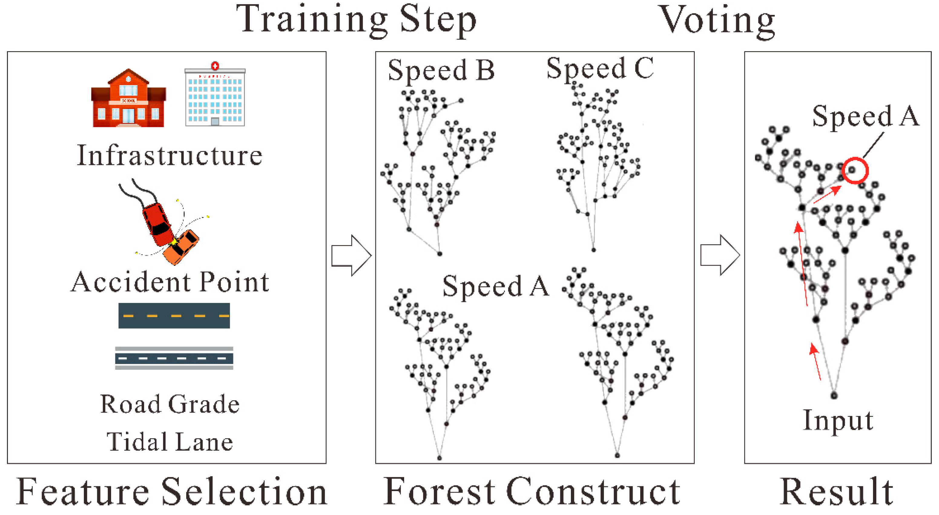
Data for unsampled road sections were derived according to the prediction results of the model established by the random forest method. The concept of the random forest model is shown in Figure 3. In this model, firstly, the factors that affect the traffic are taken as the training data input, and the random forest classifier is constructed. The result is assigned to class a through voting output, where Class A represents the driving speed of the segment.

(3) Fuzzy reasoning

The fuzzy reasoning method uses the combined weight of multiple similar typical road section samples as the weight of the unsampled road section. All samples’ information is used in the fuzzy reasoning method to evaluate the traffics for information missing road sections and can avoid them being simply classified as a single class by the random forest method. The steps for fuzzy reasoning are as follows: after the unsampled road section is predicted by the random forest method (i.e., the classification result), select the typical road section sample where the difference between the dependent variable of the typical road section sample and the classification result is within a certain threshold. Then, calculate the unsampled road section and the selected road section based on the fuzzy inference method. The similarity degree for the samples of typical road sections is combined with the fuzzy membership degree of the index to obtain the road weight of the unsampled road section. The fuzzy membership degree of the index measures the similarity degree and the speed weight. Calculate the similarity between the h-th unsampled road section and the environmental factors for each typical road section with the fuzzy inference method (see Equation (1)).

$$S_{i,h}=\frac{1}{m}{\displaystyle \sum _{j=1}^m{e}^{{\left(\frac{\left|p_{j,h}-p_{jt,h}\right|}{w_1}\right)}^{2}In(k_1)}}$$

(1)

$S_{i,h}$ represents the similarity between the h-th unsampled section and the i-th typical road section. $p_{j,h}$ represents the j-th road attribute value of the h-th unsampled section. $p_{jt,h}$ represents the j-th road attribute of each typical road section corresponding to the h-th unsampled road section, $k_1$. $w_1$ represents the correction parameters. $m$ is the number of influencing factors.

Based on the similarity between the h-th unsampled road section and each typical road section, the weight corresponding to the h-th unsampled road section is calculated using Equation (2).

$$W_h=\frac{{\displaystyle \sum _{i=1}^n{S}_{i,j}{W}_{i,h}}}{{\displaystyle \sum _{i=1}^n{S}_{i,j}}}$$

(2)

$W_h$ represents the speed weight corresponding to the h-th unsampled road section, and $W_{i,h}$ represents the speed weight of the i-th typical road section corresponding to the h-th unsampled road section. The specific steps are shown in Figure 4.

4.3. Shortest Path Impedance Setting

The impedance setting function relationship is based on the principle that as vehicle speed increases, impedance decreases. In other words, under the effect of the influence factor (e.g., tidal lane, distance to traffic units, and accident sections), the longer a trip takes, the lower the average speed and the greater the road impedance. Setting a suitable impedance can effectively avoid congested road sections in path optimization and achieve the purpose of increasing the pass rate. The mathematical basis of the impedance setting is the ratio of the road weight to road length (Equation (3)). The speed weight, under real-world conditions, is affected by changes in the length weight. Such changes also affect the results of the shortest path planning algorithm, thereby weight changes affect the impedance, and the impedance affects the result of the shortest path planning algorithm. Path planning is calculated as follows:

$$W=\frac{speed\_allowed}{speed\_inferred/actual}\cdot road\_length$$

(3)

$W$ is the road impedance used for path planning. $road\_length$ is the length of the road. $speed\_allowed$ is the different speed limits of the roads. $speed\_inferred/actual$ is the speed inferred or the actual speed, if the information of the road section is not complete, $speed\_inferred$ will used in here which is inferred from Equation (2), if the road network information is complete, $speed\_actual$ will be used here and it is the actual speed. When the road conditions are good,$w$ is the same as $speed\_allowed$. When the road conditions are poor,$w$ is smaller than $speed\_allowed$ and the impedance of the road section with poor conditions, $W$ will increase.

4.4. Network Analyst

After obtaining the full path impedance, a geometric network and a logical network are established based on the network analysis module of ArcGIS software. The geometric network comprises a series of topology-related feature classes and is a graphical representation of geographic features. Obtain the urban road network data from OpenStreetMap. The urban road geometric network model comprises two types of feature classes: the centerline of the road and the road junction. It can be established by the Create Geometric Network Tool in the ArcGIS desktop software, ArcCatalog. After checking the topology and establishing the network data set, enter the total road network impedance calculated in the previous step into the attribute database. Open the ArcToolbox of ArcGIS, select “Network Analyst Tools-Make OD Cost Matrix Layer,” enter the network data set just created, successfully build the OD matrix, and then load the starting point and ending point position, click the solution on the network analysis toolbar, and the calculation ends.

5. Experiments and Results

Three experiments were conducted for various routes in the study area during the times of, morning peak, daytime, evening peak and night. The routes had different starting and ending points. A total of 392 samples were selected for typical road sections. Sample selections considered different road characteristics.

Table 3. Sample selection categories and data statistics.

Road Grade	Time Period	Distance to Traffic Unit	Tidal Lane	Distance from the Accident-Prone Section	Number of Samples
Trunk	Morning peak	<30 m	Yes	<30 m	5
	Daytime	30–60 m	Yes	>100 m	6
	Evening peak	>100 m	Yes	>100 m	4
	Night	>100 m	No	>100 m	3
	Morning peak	>100 m	No	>100 m	4
Primary	Daytime	>100 m	No	>100 m	4
	Evening peak	<30 m	No	>100 m	8
	Night	60–100 m	No	>100 m	6
Secondary	Morning peak	30–60 m	No	60–100 m	21
	Daytime	>100 m	No	>100 m	38
	Evening peck	>100 m	No	>100 m	12
	Night	>100 m	No	>100 m	22
Third level	Morning peak	<30 m	Yes	<30 m	3
	Daytime	>100 m	No	>100 m	11
	Evening peck	>100 m	No	>100 m	4
	Night	<30 m	No	>100 m	5
Residential	Morning peak	60–90 m	No	>100 m	2
	Daytime	<30 m	No	>100 m	6
	Evening peck	30–60 m	No	30–60 m	3
	Night	30–60 m	No	>100 m	4

shows the sample selection process.

A total of two tests were carried out for the whole area of the study area. For the first time, a total of three groups were tested to study the practical application of the fuzzy random forest algorithm when the road information is not covered. The selected time periods for the three groups of tests are morning peak (Figure 5a), daytime (Figure 5b) and night (Figure 5c), and different starting and ending points are selected. When there was missing traffic information for a given road section, we set the impedance to the speed limit allowed by the road class. (a2, b2, c2) and the whole road network data inferred by the fuzzy random forest as the impedance (a1, b1, c1) test, respectively; at the same time, statistics on the coverage and lack of traffic information in this period (a3, b3, c3); the path results are shown in Figure 5. Calculate the parameters of the first group and the results are compared in the following table. The shortest path in

Table 4. Comparison of the statistics of the Test 1 path algorithm results.

Path	Path by out Method	Shortest Path
Path length (km)	19.35	18.52
Average speed (km/h)	35.50	32.14
Evaluation of travel time (min)	32.69	34.57
Time period	Morning peak	Morning peak
Primary	3	2
Secondary	4	5
Third level	0	0

refers to the shortest distance calculated with the road length as the impedance. Although the path is the shortest, due to the traffic congestion at that time, the average speed of the shortest path is lower and the travel time is longer than the path by our method.

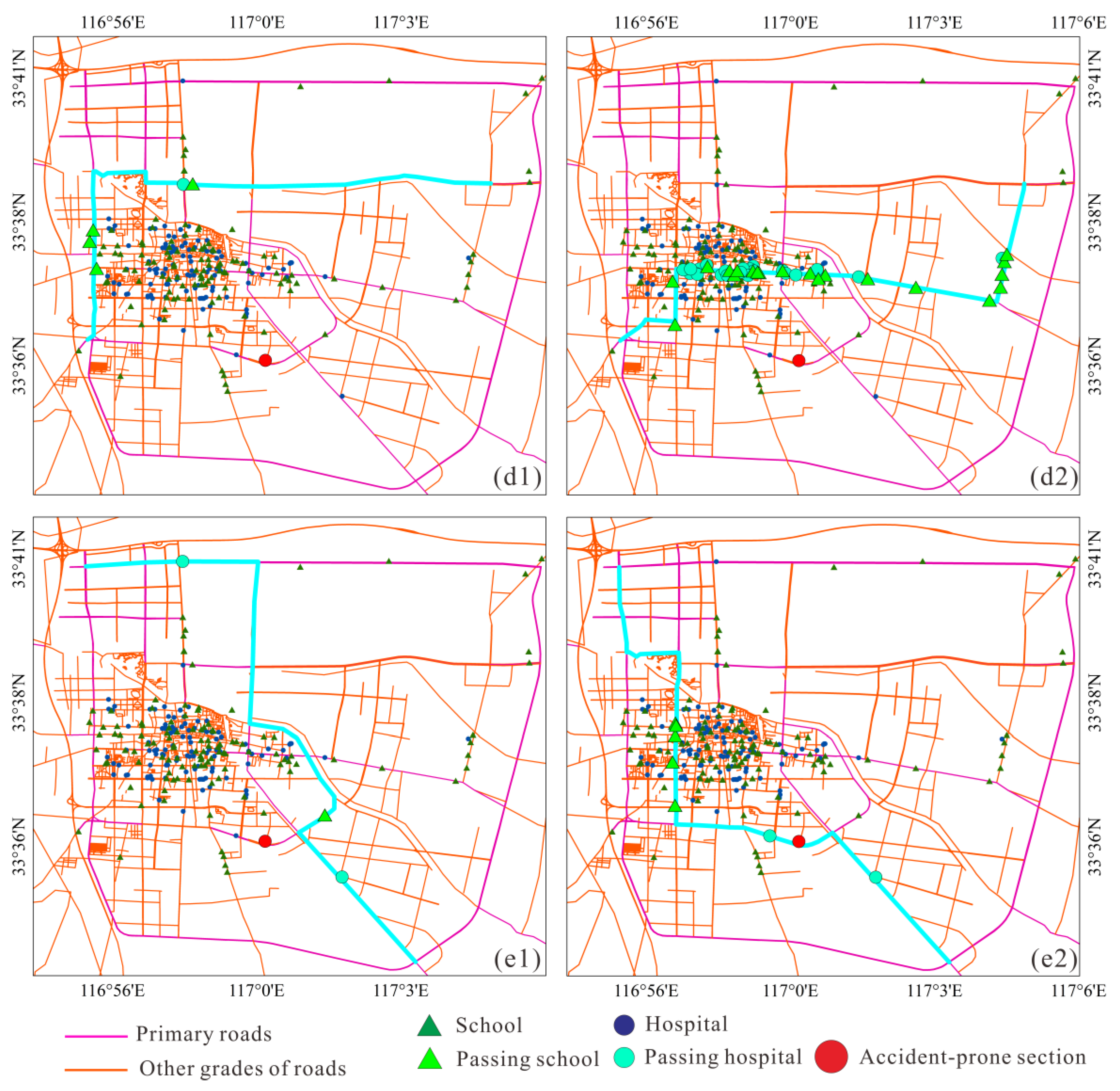
In the second test, two groups were tested. The selected time periods were morning peak (Figure 6d) and evening peak (Figure 6e), and different starting points and ending points were selected. Use the speed limit allowed by the road class as the impedance (d2, e2) and the whole road network data inferred by the fuzzy random forest as the impedance (d1, e1) test. At the same time, count the schools, hospitals and accident road sections passed by during the driving process, and calculate. The first two groups of parameters are compared in the following

Table 5. Comparison of the statistics of the Test 2 path algorithm results.

Method	Path by out Method	Shortest Path
Path length (km)	24.26	23.30
Average speed (km/h)	36.52	33.28
Evaluation of travel time (min)	39.85	42.00
Time period	Evening peak	Evening peak
School	1	5
Hospital	2	2
Accident section	0	1

:

According to the result of the regional route’s planned length, the planned route passes through the static impedance and entered the city’s core. Using fuzzy impedance, the path planning result avoided roads in the city. Although the total travel distance increased slightly, the ratio of fast-driving roads to slow-driving roads was higher. The estimated travel time was also shorter. This route is also more in line with actual driving habits, indicating that the impedance model based on fuzzy inference has practical application value.

Urban road networks do not have complete traffic information covering the whole of the network. Traditional methods set the impedances of road sections with missing traffic information to their speed limits. Practically, vehicles driving on a given road often do not hit the road’s speed limit. Using a fuzzy random forest model to estimate traffic data for road sections with missing traffic information can give more accurate estimates of the average driving speed on these road sections for a given time period. Consequently, the road network can be considered to have full traffic information coverage. On this basis, travel route optimization decisions that better reflect the real road conditions during a given period can be made. In the test, the fuzzy random forest method avoided the nodes in the urban core area where the theoretical value of speed limit is very high, such as schools and hospitals, but are actually congested. The result of path optimization increases the average speed during road driving process at a cost of only approximately 5% of the increased distance traveled, which ultimately reduces the driving time, greatly improves driving comfort, and has evident advantages.

6. Discussion

Since it is difficult just using an equation to calculate the weights covering the whole road links directly, this paper brings out a new model to estimate the impedance of the path based on a fuzzy random forest. This study mainly focuses on generating the complete and symmetrical road network coverage data based on the existing GPS data, which are used for path planning considering time. The planning result is more reasonable during the traffic peak period than using the default impedance directly when there is no GPS data coverage. Analyzing and quantifying the factors affecting traffic is a crucial issue. Whole and detailed factors can improve the accuracy of routing. The factors chosen depend on expert knowledge. Factors affecting traffic in different regions may be different.

In further research, we will apply the method to other research areas. First of all, the characteristics of different regions need to be considered to select the appropriate impact factors. For example, in areas with large terrain differences, elevation change, and snow are important. Secondly, the same factors in different regions may have different actual effects, and the weight can be adjusted according to the actual situation of different countries. In the following research, we will apply the incomplete information network construction method to other areas with high-frequency GPS data, which needs to consider other factors.

7. Conclusions

Weights covering all road links are the basis of routing. Traditional methods have difficulty generating accurate impedances for road links with incomplete traffic information. Using historical GPS trajectory data, this paper proposes a new road network weight distribution method based on a fuzzy random forest model. This method introduces the third law of geography into the distribution of road weights. It estimates the average driving speeds for roads with missing traffic information by constructing a mapping relationship between the average road speed and the internal and external factors that affect road traffic. Experimental results showed that this method is effective. Analysis of the traffic impact factors, and their quantifications are key to this method. Complete and detailed knowledge of the factors that affect routing can improve routing accuracy. The relationships between such factors and traffic are also important. This paper introduces several factors that affect traffic.

Choosing the appropriate environmental factors for sample selection, and the subsequent training of a fuzzy random forest model using those samples, is important in order to obtain the driving speed of the entire road network. When the fuzzy random forest algorithm is used to interpolate the data for road networks with unknown driving information, in view of, the selection of influencing factors is not set in stone due to the complex factors that affect driving speed and its many aspects. Different cities have different traffic-affecting factors. The calculation of road weights depends on the attributes of the roads. Therefore, the influencing factors of representative roads in different cities can be analyzed and tested, and the results obtained can further enrich and perfect this method.