A Fuzzy Optimization Technique for Multi-Objective Aspirational Level Fractional Transportation Problem

Abstract

In this research work, a soft computing optimization operating approach is developed for a multi-objective aspirational level fractional transportation problem. In the proposed technique, a mathematical model is formulated for the multi-objective aspirational level fractional transportation problem (MOFTP) based on the highest value of one and all objectives of the model. We also used the symmetry concept over our model to identify the best optimum solution based on symmetrical data. We constructed the membership grades for the set of fetched parameters having symmetry. In this work, we also used the concept of ranking function in our mathematical model to obtain the optimum solution of the fuzzy multi-objective fractional transportation. In this proposed algorithm, the aspiration levels are also associated with the objective function of MOFTP. We are also proposing a new approach for the optimization of fractional problems in which the objectives are being optimized by using the numerator function and denominator function simultaneously. Further, a methodology is also developed to find the average cost for each fractional objective of the model. After that, we will find the ranking function for each parameter by using the defuzzification method. By this methodology, we will be able to convert the MOFTP into a bi-objective transportation problem. The provided technique is elaborated with the help of numerical computations to prove the beauty and power of the proposed technique.

1. Introduction

Commodities from one point to another are shifted at a lower cost within less time. These problems are acknowledged as transportation problems. The transportation problem was first introduced by Hitchcock [1] in 1941. In such a problem, a fixed commodity is shifted from a finite number of origins to a finite number of targets to fulfill the requirement of the system. Such types of transportation problems are known as classical transportation problems. Again, the concepts of classical transportation problems were discussed by Koopmans [2] in 1949. The transportation problem has many real-life applications, such as in practical transport [3], trip planning [4], and last-mile logistics [5]. There are various techniques such as Vogel’s Approximation Method, Least Cost Method, and North West Corner Rule to obtain the basic feasible solution in the context of the transportation problems. To obtain the ideal solution to the transportation problems, the well-known MODI method is used. Many approaches exist in the literature to obtain the optimal solution for transportation problems. The simplex method is also used to solve the transportation problems by changing the problem into a linear programming problem. However, due to the complex structure of the Simplex method, it is not always acceptable to solve transportation problems. Therefore, there is a need to improve the existing methods available for the optimal solution to transportation problems. Goyal [6] also provided a methodology for the improvement in Vogel’s approximation method for the solution of the unbalanced transportation problem.

In the classical transportation problems, entire parameters such as transport cost, accessibility of sources, and demand of destination are known and fixed. However, in real-life situations, some parameters are not exact due to various reasons such as road damage on rainy days affect the transport cost. When a new product is launched, it affects the demand for an old product. Suddenly by emailing or through an online system, anyone can change the demand, which affects the supply chain of the supplier. Therefore, this causes uncertainty in these parameters. The classical methods are insufficient to cover up all the uncertainties in the parameters that affect the transportation problem. Fuzzy logic is applied to trade in with these types of uncertain transportation problems; such types of transportation problems are known as Fuzzy Transportation Problems. For the mathematical representation of this uncertainty or vagueness, Zadeh [7], in 1965, introduced a theory that is known as fuzzy set theory. In 1970, Bellman and Zadeh [8] used this theory for decision-making problems, and then Oheigeartaigh [9] used this theory in transportation problems with fuzzy parameters.

Yager [10] introduced an extension principle of fuzzy sets to represent the mappings of relations. Moreover, in real problems, everyone wants to decide on the multi-objectives that can be optimized by the nature of the decision. Every decision-maker wants to fulfill the demand of the destination at minimum cost, minimum time, maximum profit, and minimum effort with minimum damages due to confliction in incommensurable objectives. With this aspect, transportation problems were extended to multi-objective transportation problems (MOTP). This is impossible to find an ideal solution for all objectives simultaneously. To obtain the solution to such problems, various techniques such as Goal programming, Fuzzy programming, Geometric programming approaches, Quadratic programming, and Genetic algorithm are used to obtain the compromise ideal solution satisfying all the objectives. When a fuzzy transportation problem involves more than one objective function, then the task to find out one or more optimal solutions is known as fuzzy programming for the multi-objective transportation problem. Zimmermann [11] discussed fuzzy programming for multi-objective problems. Balan [12] used fuzzy programming to obtain the multi-objectives of fuzzy linear optimization. Bit et al. [13] gave a solution to a multi-criteria decision-making transportation problem by using fuzzy programming, and Bit et al. [14,15] also used the fuzzy system to obtain the ideal solution of a multi-objective solid transportation problem and for capacitated multi-objective transportation problems. Verma et al. [16] provided the compromise optimal solution methodology by using the fuzzy technique for multi-objective transportation difficulties with non-linear membership function, then Bit [17] provided a solution for multi-objective capacitated transportation problem with hyperbolic membership functions by using fuzzy programming. T. Zeng and Huang [18] provided the mathematical tools for multiple objective decisions making in a fuzzy environment. Singh and Singh [19] gave a new technique for the solution of a bi-objective transportation problem.

In transportation problems, when the objective function is given in the proportion of two linear functions is known as a Fractional Transportation Problem (FTP). In these problems, the objective function may be a proportion of two cost functions or two objective functions. Whenever more than one objective is enhanced in the FTP at that time, this problem is called MOFTP. Charnes and Cooper [20] worked out linear fractional functions and provided programming for these types of functions. Swarup [21] studied linear fractional functional programming for transportation problems. Kornbluth and Steuer [22] introduced linear fractional programming with multiple objectives. Luhandjula [23] used fuzzy logic for the optimization of linear fractional problems with multiple objectives. Dutta et al. [24] used the fuzzy set theory to find effective solutions to multi-objective linear fraction programming difficulties, and also, [25] used the fuzzy approach for the optimization of multi-criteria linear fractional problems. Joshi and Gupta [26] dealt with the condition of variation in demand and supply for linear fractional transportation problems. Dangwal et al. [27] gave a goal programming approach to find the suitable ideal solution of the multi-objective linear fractional problem in a vague environment. Sadia et al. [28,29] worked on multi-objective fractional problems by taking the capacitated transportation problem with mixed and uncertain constraints, i.e., in a fuzzy environment. Maruti [30] provided a solution procedure for solving MOFTP. Sheikhi et al. [31] also provided a method aimed at the solution of the multi-objective transportation problems in which two objectives are taken, i.e., a bi-objective transportation problem. Then, Anukokila et al. [32] gave a new approach by using goal programming to find the optimal conciliation solution for multi-objective fractional transportation problems. Goal programming-based articles were also studied to solve solid transportation problems [33] and multi-criteria decision-making problems [34]. Das et al. [35] used the fully fuzzy linear fractional programming problems based on multi-objective linear programming. Mehrjerdi [36] introduced the concept of fractional programming problems through fuzzy goal settings and approximation. Gessesse et al. [37] provided the genetic algorithm-based fuzzy programming approach for multi-objective linear fraction stochastic transportation problems with four-parameter Burr distribution. Quadratic programming [38] with fuzzy parameters was also studied in which a membership function-based approach is used to handle the problem. In this paper, we define an algorithm that was projected for the multi-objective fractional transportation problem. In this work, first, we introduced the ranking function for the fuzzy parameters. We also proposed a method for converting the multi-objective fractional transportation problem into the bi-objective problem by dealing with the numerator and denominator. We also proposed the aspiration level for each objective. The proposed algorithm is more effective and quite easy to use with less computation. Furthermore, we also used symmetrical data to perform the symmetry [39,40] concept over the proposed approach. Results in a variation by taking symmetrical and non-symmetrical data were illustrated through this proposed technique. In this present research paper, we developed a model based on the aspirational level to solve multi-objective fractional transportation in a fuzzy environment, which provides a more optimal solution than the other existing studies.

The present work is categorized into six sections. In the second section, we gave some preliminaries linked with our work. In this section, we also introduced the aspiration level for the fuzzy multi-objective fractional transportation problem. In the third section, we introduced our approach based on ranking function and aspiration level through an algorithm that is more effective and less time-consuming; the architecture of the proposed algorithm was also provided in this section. In the fourth section, we gave a numerical example to check the efficiency of our proposed approach for MOFTP. In the fifth section, we compared the validation of our proposed approach with the existing method and our proposed approach. In the last section, we discussed the deduction of the entire work.

2. Some Preliminaries

2.1. Fuzzy Set

Let U be a universal set, then a set $\tilde{\mathrm{F}}$ is said to be a fuzzy set of set U if a membership function ${\mathsf{\mu }}_{\tilde{\mathrm{F}}}$ is defined such that ${\mathsf{\mu }}_{\tilde{\mathrm{F}}}\left(\mathrm{u}\right)$: $\tilde{\mathrm{F}}\to \left[0,1\right]$, $\forall \mathrm{u}\in \mathrm{U}$, where ${\mathsf{\mu }}_{\tilde{\mathrm{F}}}\left(\mathrm{u}\right)$ is the membership grade of $\mathrm{u}\in \mathrm{U}$ in $\tilde{\mathrm{F}}$ and its value of ${\mathsf{\mu }}_{\tilde{\mathrm{F}}}\left(\mathrm{u}\right)$ lies between 0 and 1. This fuzzy set $\tilde{\mathrm{F}}$ is represented by

$$\tilde{\mathrm{F}}=\left\{\left( \mathrm{u},{\mathsf{\mu }}_{\tilde{\mathrm{F}}}\left(\mathrm{u}\right)\right): \mathrm{u}\in \mathrm{U}\right\}$$

(1)

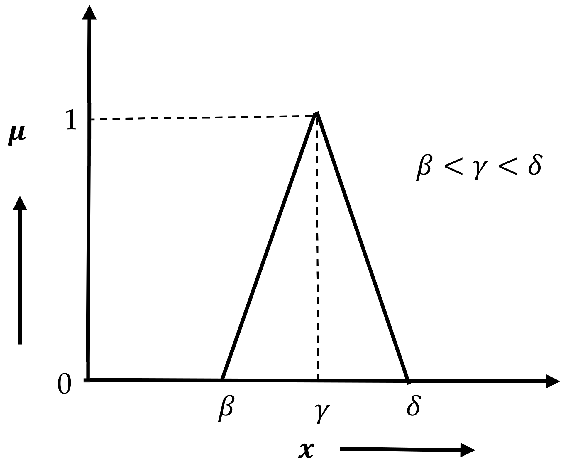
2.2. Fuzzy Number

A fuzzy set $\tilde{\mathrm{F}}$ on a real line $\mathrm{R}$ is said to be a fuzzy number if fuzzy set $\tilde{\mathrm{F}}$ propitiates the following properties:

• Height of fuzzy set $\tilde{\mathrm{F}}$ must be 1;
• Support of $\tilde{\mathrm{F}}$ must be bounded on $\mathrm{R}$;
• Every $\mathrm{alpha} \mathrm{cut} \mathrm{set}$ of $\tilde{\mathrm{F}}$ should be a closed interval for each $\mathsf{\alpha }\in$ [0,1].

A geometric representation of a triangular fuzzy number is provided in Figure 1. In which the values $\mathsf{\beta }, \mathsf{\gamma }, \mathsf{\delta }$ belong to real line $\mathrm{R}$ and the maximum membership value $\mathsf{\mu }$ is 1.

2.3. Triangular Fuzzy Number

A fuzzy number $\tilde{\mathrm{F}}$ represented by a set $\left(\mathsf{\beta }, \mathsf{\gamma }, \mathsf{\delta }\right)$ is called triangular type fuzzy number if its membership function is represented, as shown in Figure 1.

$${\mathsf{\mu }}_{\tilde{\mathrm{F}}}\left(\mathrm{u}\right) = \left\{\begin{array}{c}0, \mathrm{u}\le \mathsf{\beta } \mathrm{and} \mathrm{u}\ge \mathsf{\delta }\\ \frac{\mathrm{u}-\mathsf{\beta }}{\mathsf{\gamma }-\mathsf{\beta }}, \mathsf{\beta }\le \mathrm{u}\le \mathsf{\gamma }\\ \frac{\mathsf{\delta }-\mathrm{x}}{\mathsf{\delta } - \mathsf{\gamma }}, \mathsf{\gamma }\le \mathrm{u}\le \mathsf{\delta }\end{array}\right\}, \mathrm{where} \mathsf{\beta }<\mathsf{\gamma }<\mathsf{\delta }.$$

(2)

2.4. Ranking Function

Let $\tilde{\mathrm{F}}=\left(\mathsf{\beta }, \mathsf{\gamma }, \mathsf{\delta }\right)$ be a triangular fuzzy number.

Then the ranking function is

$$\mathrm{R}\left(\tilde{\mathrm{F}}\right)= \mathrm{R}\left(\mathsf{\beta }, \mathsf{\gamma }, \mathsf{\delta }\right)={{\displaystyle \int }}_0^{1}0.5\left({\mathrm{F}}_{\mathsf{\alpha }}^{\mathrm{L}}+{ \mathrm{F}}_{\mathsf{\alpha }}^{\mathrm{U}}\right)\mathrm{d}\mathsf{\alpha }$$

(3)

where $\left[{\mathrm{F}}_{\mathsf{\alpha }}^{\mathrm{L}},{\mathrm{F}}_{\mathsf{\alpha }}^{\mathrm{U}}\right] = \left[(\mathsf{\beta } + (\mathsf{\gamma }-\mathsf{\beta })\mathsf{\alpha }), (\mathsf{\delta }-(\mathsf{\delta }-\mathsf{\gamma })\mathsf{\alpha })\right]$, is a crisp interval for triangular fuzzy set $\tilde{\mathrm{F}}\forall \mathsf{\alpha } \in \left[0,1\right].$

2.5. Fractional Transportation Problem

The fractional transportation problem (FTP) was provided by Swarup in 1966 [21]. A fractional transportation problem is a transportation problem in which objective function is in the rational form. Let us recognize a fractional transportation problem with “p” number of sources and “q” number of destinations. Let ${\mathrm{m}}_{\mathrm{i}}$ be the number of available quantities of product at ${\mathrm{i}}^{\mathrm{th}}$ source and ${\mathrm{n}}_{\mathrm{j}}$ be the demand by ${\mathrm{j}}^{\mathrm{th}}$ target. The commodities are transported from the ${\mathrm{i}}^{\mathrm{th}}$ source to ${\mathrm{j}}^{\mathrm{th}}$ destination at the cost of ${\mathrm{s}}_{\mathrm{ij}}$ and ${\mathrm{t}}_{\mathrm{ij}}$ per unit item.

Let ${\mathrm{u}}_{\mathrm{ij}}$ be the number of products transported from ${\mathrm{i}}^{\mathrm{th}}$ source to ${\mathrm{j}}^{\mathrm{th}}$ destination.

Then, the mathematical structure of the Fractional Transportation problem as:

$$\mathrm{Min} \mathrm{Z}(\mathrm{u})=\frac{{{\displaystyle \sum }}_{\mathrm{i} =1}^{\mathrm{p}}{{\displaystyle \sum }}_{\mathrm{j} =1}^{\mathrm{q}}{\mathrm{s}}_{\mathrm{ij}}{\mathrm{u}}_{\mathrm{ij}}}{{{\displaystyle \sum }}_{\mathrm{i} =1}^{\mathrm{p}}{{\displaystyle \sum }}_{\mathrm{j} =1}^{\mathrm{q}}{\mathrm{t}}_{\mathrm{ij}}{\mathrm{u}}_{\mathrm{ij}}},$$

Subject to,

$${{\displaystyle \sum }}_{\mathrm{j} =1}^{\mathrm{q}}{\mathrm{u}}_{\mathrm{ij}} ={\mathrm{m}}_{\mathrm{i}},$$

$${{\displaystyle \sum }}_{\mathrm{i} =1}^{\mathrm{p}}{\mathrm{u}}_{\mathrm{ij}} ={\mathrm{n}}_{\mathrm{j}},$$

where ${\displaystyle \sum }_{\mathrm{i} =1}^{\mathrm{p}}{\mathrm{m}}_{\mathrm{i}}={\displaystyle \sum }_{\mathrm{j} =1}^{\mathrm{q}}{\mathrm{n}}_{\mathrm{j}}$, ${\mathrm{u}}_{\mathrm{ij}}\ge 0,$ where i = 1,2….p & j = 1,2 … q.

When the parameters are fuzzy, then the structure of the problem changes, and it becomes;

$$\mathrm{Min} \mathrm{Z}(\mathrm{u})=\frac{{{\displaystyle \sum }}_{\mathrm{i} =1}^{\mathrm{p}}{{\displaystyle \sum }}_{\mathrm{j} =1}^{\mathrm{q}}{\tilde{\mathrm{t}}}_{\mathrm{ij}}{\mathrm{u}}_{\mathrm{ij}}}{{{\displaystyle \sum }}_{\mathrm{i} =1}^{\mathrm{p}}{{\displaystyle \sum }}_{\mathrm{j} =1}^{\mathrm{q}}{\tilde{\mathrm{t}}}_{\mathrm{ij}}{\mathrm{u}}_{\mathrm{ij}}},$$

Subject to, ${\displaystyle \sum }_{\mathrm{j} =1}^{\mathrm{q}}{\mathrm{u}}_{\mathrm{ij}}\le {\tilde{\mathrm{m}}}_{\mathrm{i}}$, ${\displaystyle \sum }_{\mathrm{i} =1}^{\mathrm{p}}{\mathrm{u}}_{\mathrm{ij}}\le {\tilde{\mathrm{n}}}_{\mathrm{j}}$, where ${\displaystyle \sum }_{\mathrm{i} =1}^{\mathrm{p}}{\tilde{\mathrm{m}}}_{\mathrm{i}} \approx {\displaystyle \sum }_{\mathrm{j} =1}^{\mathrm{q}}{\tilde{\mathrm{n}}}_{\mathrm{j}}$, ${\mathrm{u}}_{\mathrm{ij}}\ge 0,$ where i = 1, 2… p & j = 1,2 … q.

2.6. Multi-Criteria Fractional Transportation Problem

When there are multiple criteria concerned for mathematical optimization for a fractional objective to be optimized simultaneously. Let us consider a fractional transportation problem with “p” number of sources and “q” number of targets. Let ${\mathrm{m}}_{\mathrm{i}}$ be the number of available quantities of product at ${\mathrm{i}}^{\mathrm{th}}$ source and ${\mathrm{n}}_{\mathrm{j}}$ be the demand by ${\mathrm{j}}^{\mathrm{th}}$ target. Let ${\mathrm{c}}_{\mathrm{ij}}^{\mathrm{k}}$ and ${\mathrm{d}}_{\mathrm{ij}}^{\mathrm{k}}$ be the cost of per unit item in ${\mathrm{k}}^{\mathrm{th}}$ objective. Let ${\mathrm{u}}_{\mathrm{ij}}$ be the number of items which are transported from ${\mathrm{i}}^{\mathrm{th}}$ source to ${\mathrm{j}}^{\mathrm{th}}$ destination.

$$\mathrm{Min} {\mathrm{Z}}_{\mathrm{k}}(\mathrm{u}) = \frac{{{\displaystyle \sum }}_{\mathrm{i} =1}^{\mathrm{p}}{{\displaystyle \sum }}_{\mathrm{j} =1}^{\mathrm{q}}{\mathrm{s}}_{\mathrm{ij}}^{\mathrm{k}}{\mathrm{u}}_{\mathrm{ij}}}{{{\displaystyle \sum }}_{\mathrm{i} =1}^{\mathrm{p}}{{\displaystyle \sum }}_{\mathrm{j} =1}^{\mathrm{q}}{\mathrm{t}}_{\mathrm{ij}}^{\mathrm{k}}{ \mathrm{u}}_{\mathrm{ij}}},$$

Subject to, ${\displaystyle \sum }_{\mathrm{j} =1}^{\mathrm{q}}{\mathrm{u}}_{\mathrm{ij}}$ = ${\mathrm{m}}_{\mathrm{i}}$, ${\displaystyle \sum }_{\mathrm{i} =1}^{\mathrm{p}}{\mathrm{u}}_{\mathrm{ij}}$ = ${\mathrm{n}}_{\mathrm{j}}$, where ${\displaystyle \sum }_{\mathrm{i} =1}^{\mathrm{p}}{\mathrm{m}}_{\mathrm{i}}={\displaystyle \sum }_{\mathrm{j} =1}^{\mathrm{q}}{\mathrm{n}}_{\mathrm{j}}$, ${\mathrm{u}}_{\mathrm{ij}}\ge 0,$ where i = 1,2 … p& j = 1,2 … q.

In fuzzy environment:

$$\mathrm{Min} {\mathrm{Z}}_{\mathrm{k}}(\mathrm{u})=\frac{{{\displaystyle \sum }}_{\mathrm{i} =1}^{\mathrm{p}}{{\displaystyle \sum }}_{\mathrm{j} =1}^{\mathrm{q}}{\tilde{\mathrm{s}}}_{\mathrm{ij}}^{\mathrm{k}}{\mathrm{u}}_{\mathrm{ij}}}{{{\displaystyle \sum }}_{\mathrm{i} =1}^{\mathrm{p}}{{\displaystyle \sum }}_{\mathrm{j} =1}^{\mathrm{q}}{\tilde{\mathrm{t}}}_{\mathrm{ij}}^{\mathrm{k}}{ \mathrm{u}}_{\mathrm{ij}}},$$

(4)

Subject to, ${\displaystyle \sum }_{\mathrm{j} =1}^{\mathrm{q}}{\mathrm{u}}_{\mathrm{ij}}\le {\tilde{\mathrm{m}}}_{\mathrm{i}}$, ${\displaystyle \sum }_{\mathrm{i} =1}^{\mathrm{p}}{\mathrm{u}}_{\mathrm{ij}}\le {\tilde{\mathrm{n}}}_{\mathrm{j}}$, where ${\displaystyle \sum }_{\mathrm{i} =1}^{\mathrm{p}}{\tilde{\mathrm{m}}}_{\mathrm{i}}\approx {\displaystyle \sum }_{\mathrm{j} =1}^{\mathrm{q}}{\tilde{\mathrm{n}}}_{\mathrm{j}}$, ${\mathrm{u}}_{\mathrm{ij}}\ge 0,$ where i = 1,2 … p& j = 1,2 … q.

2.7. Aspiration Levels

The concept of aspiration levels was introduced by Pal et al. [41] in the fuzzy goal programming approach. We defined the aspiration level in multi-objective fractional transportation problems. Let ${\mathrm{L}}_{\mathrm{k}}$ be the objective level assigned [42] to each kth objective ${\mathrm{Z}}_{\mathrm{k}}$ of the MOFTP. Then, for each objective, two cases arise;

$${\mathrm{Z}}_{\mathrm{k}}\succcurlyeq {\mathrm{L}}_{\mathrm{k}} (\mathrm{for} \mathrm{maximizing})$$

$${\mathrm{Z}}_{\mathrm{k}}\preccurlyeq {\mathrm{L}}_{\mathrm{k}} (\mathrm{for} \mathrm{minimizing})$$

where, $\succcurlyeq$ and $\preccurlyeq$ indicates the “more than” and “less than” provided by Zimmermann [11].

In this case, the MOFTP can be viewed as

Find U, Satisfy ${\mathrm{Z}}_{\mathrm{k}}\left(\mathrm{U}\right)\succcurlyeq {\mathrm{L}}_{\mathrm{k}}$

$${\mathrm{Z}}_{\mathrm{k}}\left(\mathrm{U}\right)\preccurlyeq {\mathrm{L}}_{\mathrm{k}}$$

Subject to, ${\displaystyle \sum }_{\mathrm{j} =1}^{\mathrm{q}}{\mathrm{u}}_{\mathrm{ij}}$ = ${\mathrm{m}}_{\mathrm{i}}$, ${\displaystyle \sum }_{\mathrm{i} =1}^{\mathrm{p}}{\mathrm{u}}_{\mathrm{ij}}$ = ${\mathrm{n}}_{\mathrm{j}}$, where ${\displaystyle \sum }_{\mathrm{i} =1}^{\mathrm{p}}{\mathrm{m}}_{\mathrm{i}}={\displaystyle \sum }_{\mathrm{j} =1}^{\mathrm{q}}{\mathrm{n}}_{\mathrm{j}}$, ${\mathrm{u}}_{\mathrm{ij}}\ge 0,$ where i = 1,2 … p & j = 1,2 … q.

The achievement of each objective up to its aspiration level is representing the actual attainment of its corresponding membership value to the maximum possible value. Mohamed [43] defined the flexible membership goal in a fuzzy environment for aspiration level 1.

2.8. Fuzzy Programming for Multi-Objective Transportation Problem

Multi-objective transportation problem with “K” number of objectives, p number of sources, and “q” number of targets. Let ${\mathrm{m}}_{\mathrm{i}}$ be the available amount at ${\mathrm{i}}^{\mathrm{th}}$ source and ${\mathrm{n}}_{\mathrm{j}}$ be demand of ${\mathrm{j}}^{\mathrm{th}}$ destination. Then the model of fuzzy programming for multi-objective transportation problem is:

Min F, F $\le {\mathsf{\mu }}_{\mathrm{k}}\left({\mathrm{Z}}_{\mathrm{k}}\left(\mathrm{u}\right)\right)$, where ${\mathsf{\mu }}_{\mathrm{k}}$ be the membership function for ${\mathrm{k}}^{\mathrm{th}}$ objective function, and k = 1, 2 …...K, Subject to, ${\displaystyle \sum }_{\mathrm{j} =1}^{\mathrm{q}}{\mathrm{u}}_{\mathrm{ij}}\le {\tilde{\mathrm{m}}}_{\mathrm{i}}$, ${\displaystyle \sum }_{\mathrm{i} =1}^{\mathrm{p}}{\mathrm{u}}_{\mathrm{ij}}\le {\tilde{\mathrm{n}}}_{\mathrm{j}}$, where ${\displaystyle \sum }_{\mathrm{i} =1}^{\mathrm{p}}{\tilde{\mathrm{m}}}_{\mathrm{i}}\approx {\displaystyle \sum }_{\mathrm{j} =1}^{\mathrm{q}}{\tilde{\mathrm{n}}}_{\mathrm{j}}$, and $0\le$ F $\le 1$, ${\mathrm{u}}_{\mathrm{ij}}\ge 0$.

Further, we can define the aspiration levels for the fuzzy programming for MOTP, and then the given problem can be formulated as

Find U, Satisfy ${\mathsf{\mu }}_{\mathrm{k}}\left({\mathrm{Z}}_{\mathrm{k}}\left(\mathrm{u}\right)\right)\succcurlyeq {\mathrm{L}}_{\mathrm{k}}$, ${\mathsf{\mu }}_{\mathrm{k}}\left({\mathrm{Z}}_{\mathrm{k}}\left(\mathrm{u}\right)\right), \preccurlyeq {\mathrm{L}}_{\mathrm{k}}$, Subject to, ${\displaystyle \sum }_{\mathrm{j} =1}^{\mathrm{n}}{\mathrm{u}}_{\mathrm{ij}}$ = ${\mathrm{m}}_{\mathrm{i}}$, ${\displaystyle \sum }_{\mathrm{i} =1}^{\mathrm{p}}{\mathrm{u}}_{\mathrm{ij}}$ = ${\mathrm{n}}_{\mathrm{j}}$, where ${\displaystyle \sum }_{\mathrm{i} =1}^{\mathrm{p}}{\mathrm{m}}_{\mathrm{i}}={\displaystyle \sum }_{\mathrm{j} =1}^{\mathrm{q}}{\mathrm{n}}_{\mathrm{j}}$, ${\mathrm{u}}_{\mathrm{ij}}\ge 0,$ where $\mathrm{i} =1, 2\dots \mathrm{p}, \mathrm{j} =1, 2\dots \mathrm{q}$.

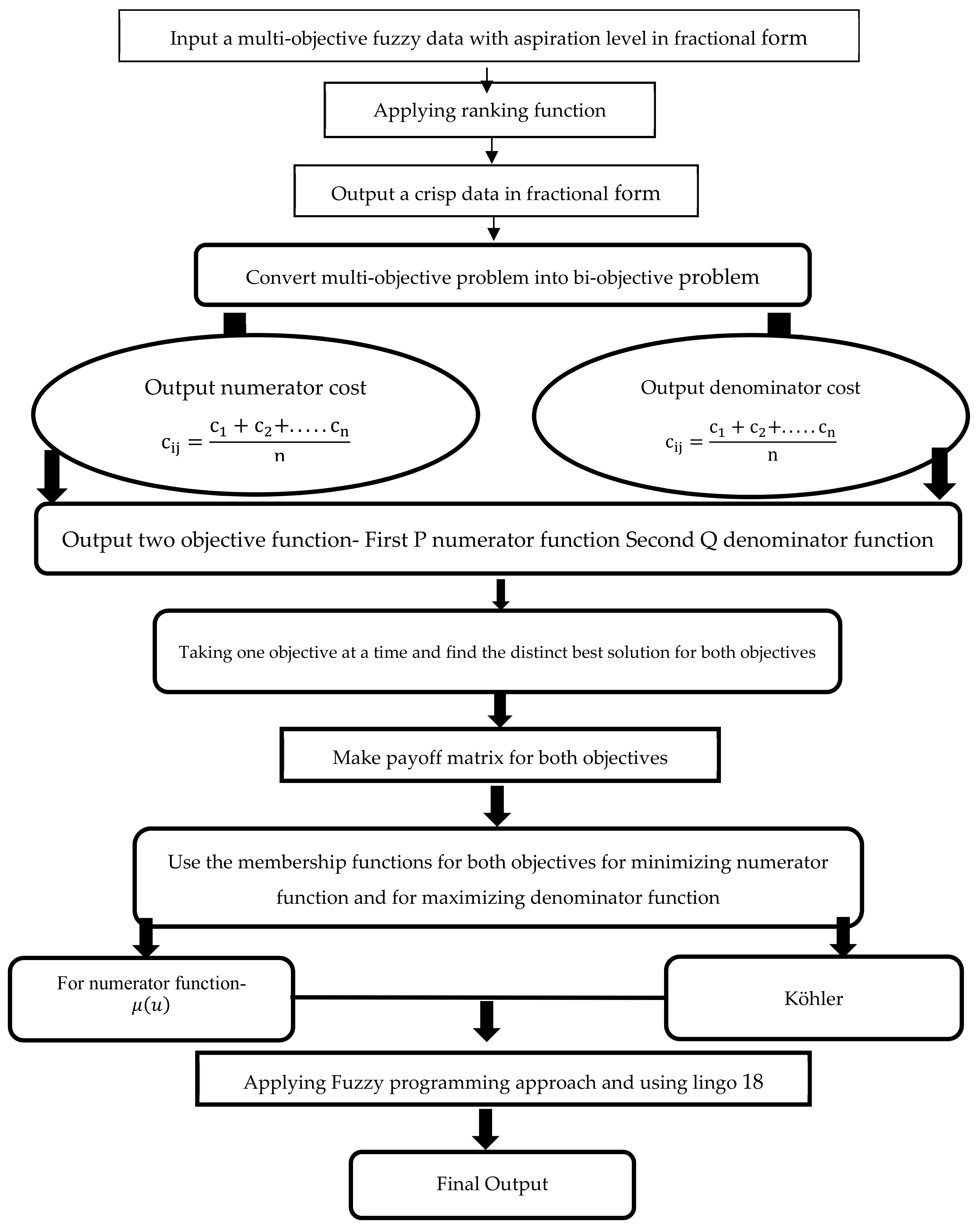
3. Proposed Algorithm for Multi-Objective Fractional Transportation Problem

Step 1: Initially, we consider a multi-objective aspirational level fractional transportation problem with fuzzy parameters. Then, convert these fuzzy parameters into crisp form with the help of a newly defined ranking function.

Formulation of the problem for aspiration levels is viewed as

Find U, Satisfy ${\mathrm{Z}}_{\mathrm{k}}\left(\mathrm{U}\right)\succcurlyeq {\mathrm{L}}_{\mathrm{k}}$, ${\mathrm{Z}}_{\mathrm{k}}\left(\mathrm{U}\right)\preccurlyeq {\mathrm{L}}_{\mathrm{k}}$, Subject to, ${\displaystyle \sum }_{\mathrm{j} =1}^{\mathrm{q}}{\mathrm{u}}_{\mathrm{ij}}$ = ${\mathrm{m}}_{\mathrm{i}}$, ${\displaystyle \sum }_{\mathrm{i} =1}^{\mathrm{p}}{\mathrm{u}}_{\mathrm{ij}}$ = ${\mathrm{n}}_{\mathrm{j}}$, where, ${\displaystyle \sum }_{\mathrm{i} =1}^{\mathrm{p}}{\mathrm{m}}_{\mathrm{i}}={\displaystyle \sum }_{\mathrm{j} =1}^{\mathrm{q}}{\mathrm{n}}_{\mathrm{j}}$, ${\mathrm{u}}_{\mathrm{ij}}\ge 0,$ Where, i = 1,2 … p & j = 1,2 … Q, $0\le \mathrm{F}\le 1$, ${\mathrm{u}}_{\mathrm{ij}}\ge 0$.

Step 2: Now, take the numerator of all objectives and find the average of corresponding costs of each numerator of all objectives and perform the same process for the denominator of all objectives. Then, convert the multi-objective aspirational level problem into a bi-objective aspirational level problem in which one objective function is minimizing function, and the other is maximizing function.

Step 3: Take one objective at a time and find the distinct best solution for both objectives and make a pay-off matrix for these objectives, as shown in

Table 1. The pay-off matrix for these objectives.

	$U_1$	$U_2$
P	${\left(\mathrm{P}\right)}_{{\mathrm{atX}}_1}$	${\left(\mathrm{P}\right)}_{{\mathrm{atX}}_2}$
Q	${\left(\mathrm{Q}\right)}_{{\mathrm{atX}}_1}$	${\left(\mathrm{Q}\right)}_{{\mathrm{atX}}_2}$

. Then, find the lower and upper bounds for both objectives.

Step 4: Now, use the membership functions $\mathsf{\mu }\left(\mathrm{u}\right)$ and $\mathsf{\vartheta }\left(\mathrm{u}\right)$ for minimizing and maximizing objective functions, respectively. $\mathsf{\mu }\left(\mathrm{u}\right)$ and $\mathsf{\vartheta }\left(\mathrm{u}\right)$ can be explicit as

$$\mathsf{\mu }\left(\mathrm{u}\right)=\left\{\begin{array}{c}1, \mathrm{if} \mathrm{P}\left(\mathrm{u}\right) \le {\mathrm{L}}_{\mathrm{P}}\\ \frac{{\mathrm{U}}_{\mathrm{P}}-\mathrm{P}\left(\mathrm{u}\right)}{{\mathrm{U}}_{\mathrm{P}}-{\mathrm{L}}_{\mathrm{P}}}, \mathrm{if} {\mathrm{L}}_{\mathrm{P}}\le \mathrm{P}\left(\mathrm{u}\right)\le {\mathrm{U}}_{\mathrm{P}}\\ 0, \mathrm{if} \mathrm{P}\left(\mathrm{u}\right)\ge {\mathrm{U}}_{\mathrm{P}}\end{array}\right\}$$

(5)

and

$$\mathsf{\vartheta }\left(\mathrm{u}\right)=\left\{\begin{array}{c}1, \mathrm{if} \mathrm{Q}\left(\mathrm{u}\right) \ge {\mathrm{U}}_{\mathrm{Q}}\\ \frac{\mathrm{Q}-{\mathrm{L}}_{\mathrm{Q}}\left(\mathrm{u}\right)}{{\mathrm{U}}_{\mathrm{Q}}-{\mathrm{L}}_{\mathrm{Q}}}, \mathrm{if} {\mathrm{L}}_{\mathrm{Q}}\le \mathrm{Q}\left(\mathrm{u}\right)\le {\mathrm{U}}_{\mathrm{Q}}\\ 0, \mathrm{if} \mathrm{Q}\left(\mathrm{u}\right)\le {\mathrm{L}}_{\mathrm{Q}}\end{array}\right\}$$

(6)

where ${\mathrm{U}}_{\mathrm{P}}$ and ${\mathrm{L}}_{\mathrm{P}}$ are the upper and lower values for minimizing the objective function, respectively, and ${\mathrm{U}}_{\mathrm{Q}}$ and ${\mathrm{L}}_{\mathrm{Q}}$ are the upper and lower values for maximization of the objective function.

Step 5: Then, for finding the best compromise solution of each objective simultaneously for MOFTP, use the fuzzy programming approach. First, we formulate the mathematical structure of our proposed model

Max F; for minimizing function: F $\le \mathsf{\mu }\left(\mathrm{u}\right)$ where $\mathsf{\mu }\left(\mathrm{u}\right)$ = $\frac{{\mathrm{U}}_{\mathrm{P}}-\mathrm{P}\left(\mathrm{u}\right)}{{\mathrm{U}}_{\mathrm{P}}-{\mathrm{L}}_{\mathrm{P}}}$; i.e., $\mathrm{P}\left(\mathrm{u}\right)\le {\mathrm{U}}_{\mathrm{P}}-$ A∗(${\mathrm{U}}_{\mathrm{P}}-{\mathrm{L}}_{\mathrm{P}}$), where ${\mathrm{U}}_{\mathrm{P}}{ \mathrm{and} \mathrm{L}}_{\mathrm{P}}$ are upper and lower bound for minimizing an objective function.

For maximizing function: F $\le \mathsf{\vartheta }$ (u) where $\mathsf{\vartheta }\left(\mathrm{u}\right)$ = $\frac{\mathrm{Q}-{\mathrm{L}}_{\mathrm{Q}}\left(\mathrm{u}\right)}{{\mathrm{U}}_{\mathrm{Q}}-{\mathrm{L}}_{\mathrm{Q}}}$; i.e., $\mathrm{Q}\left(\mathrm{x}\right)\ge$ F∗(${\mathrm{U}}_{\mathrm{Q}}-{\mathrm{L}}_{\mathrm{Q}}$) + ${\mathrm{L}}_{\mathrm{Q}}$, where ${\mathrm{U}}_{\mathrm{Q}}{ \mathrm{and} \mathrm{L}}_{\mathrm{Q}}$ are upper and lower bound for maximizing the objective function.

Subject to; ${\displaystyle \sum }_{\mathrm{j} =1}^{\mathrm{q}}{\mathrm{u}}_{\mathrm{ij}}\le {\mathrm{m}}_{\mathrm{i}}$, ${\displaystyle \sum }_{\mathrm{i} =1}^{\mathrm{p}}{\mathrm{u}}_{\mathrm{ij}}\le {\mathrm{n}}_{\mathrm{j}}$,

Step 6: Lingo 18 software (LINGO is the best tool to solve the linear, non-linear, quadratic, semi-definite, and many other optimization models easily and quickly) is used to obtain the numerical computations. We obtain the values of each ${\mathrm{x}}_{\mathrm{ij}}$ and then find the value of each objective for the multi-objective aspirational level fractional transportation problem. If the decision-maker is not satisfied with the results, then move forward to step 7.

Step 7: After obtaining the solution by fuzzy programming approach, if the conclusion maker is not fulfilled by the obtained value of these three, i.e., cost, time, and depreciation for the objectives of MOFTP, then change lower bound for maximizing function by the new value of that function. We again resolve the problem and obtain the best suitable compromised (shown in Figure 2) ideal solution for the problem.

4. Numerical Example

In this section, we computed two numerical examples, one is based on non-symmetrical data, and the other is based on symmetrical data. We take an example (for non-symmetrical data) from Sadiaet al. [29] for multi-objective aspirational level fractional transportation problems in a fuzzy environment and use the membership function of [44]. We then check the efficiency of our proposed approach over the existing approach [29].

Step 1: The fuzzy cost matrix of the entire objectives is presented in tabular form in

Table 2. First objective ${\mathrm{Z}}_1$ (Fuzzy cost) matrix.

	$n_1$	$n_2$	$n_3$
$m_1$	$\frac{\left(3,5,7\right)}{\left(1,3,5\right)}$	$\frac{\left(4,7,8\right)}{\left(1,4,5\right)}$	$\frac{\left(14,15,17\right)}{\left(11,13,15\right)}$
$m_2$	$\frac{\left(6,8,10\right)}{\left(11,12,15\right)}$	$\frac{\left(14,17,18\right)}{\left(12,14,16\right)}$	$\frac{\left(11,12,13\right)}{\left(5,7,8\right)}$
$m_3$	$\frac{\left(12,14,16\right)}{\left(12,15,16\right)}$	$\frac{\left(7,10,11\right)}{\left(4,6,8\right)}$	$\frac{\left(11,13,14\right)}{\left(6,8,9\right)}$

,

Table 3. Second objective ${\mathrm{Z}}_2$ (Fuzzy time) matrix.

	$n_1$	$n_2$	$n_3$
$m_1$	$\frac{\left(15,17,18\right)}{\left(7,9,12\right)}$	$\frac{\left(3,5,6\right)}{\left(1,2,4\right)}$	$\frac{\left(8,10,12\right)}{\left(0,3,4\right)}$
$m_2$	$\frac{\left(0,1,4\right)}{\left(1,2,5\right)}$	$\frac{\left(8,11,12\right)}{\left(3,4,5\right)}$	$\frac{\left(4,6,7\right)}{\left(3,5,6\right)}$
$m_3$	$\frac{\left(10,13,14\right)}{\left(6,8,10\right)}$	$\frac{\left(15,16,17\right)}{\left(10,12,13\right)}$	$\frac{\left(9,10,13\right)}{\left(9,11,14\right)}$

and

Table 4. Third Objective ${\mathrm{Z}}_3$ (Fuzzy vandalization imputation) matrix.

	$n_1$	$n_2$	$n_3$
$m_1$	$\frac{\left(10,13,14\right)}{\left(6,8,11\right)}$	$\frac{\left(13,15,16\right)}{\left(7,9,10\right)}$	$\frac{\left(6,8,9\right)}{\left(9,11,12\right)}$
$m_2$	$\frac{\left(13,15,16\right)}{\left(9,11,12\right)}$	$\frac{\left(13,14,15\right)}{\left(4,6,8\right)}$	$\frac{\left(15,19,21\right)}{\left(5,7,8\right)}$
$m_3$	$\frac{\left(4,7,8\right)}{\left(6,9,10\right)}$	$\frac{\left(13,15,16\right)}{\left(4,6,7\right)}$	$\frac{\left(15,17,18\right)}{\left(6,7,9\right)}$

.

Supply: ${\mathrm{m}}_1$ = 12, ${\mathrm{m}}_2$ = 15, ${\mathrm{m}}_3$ = 20,

Demand: ${\mathrm{n}}_1$ = 9, ${\mathrm{n}}_2$ = 13, ${\mathrm{n}}_3$ = 21.

For first objective function costs:

$$\begin{array}{c}\mathrm{R}({\tilde{\mathrm{c}}}_{11}^{\mathrm{q}})=5, \mathrm{R}({\tilde{\mathrm{c}}}_{12}^{\mathrm{q}})=6.5, \mathrm{R}({\tilde{\mathrm{c}}}_{13}^{\mathrm{q}})=15.25, \mathrm{R}({\tilde{\mathrm{c}}}_{21}^{\mathrm{q}})=8, \mathrm{R}({\tilde{\mathrm{c}}}_{22}^{\mathrm{q}})=16.5, \mathrm{R}({\tilde{\mathrm{c}}}_{23}^{\mathrm{q}})=12, \mathrm{R}({\tilde{\mathrm{c}}}_{31}^{\mathrm{q}})=14, \mathrm{R}({\tilde{\mathrm{c}}}_{32}^{\mathrm{q}})=9.5, \mathrm{R}({\tilde{\mathrm{c}}}_{33}^{\mathrm{q}})=\\ 12.75.\mathrm{R}({\tilde{\mathrm{c}}}_{11}^{\mathrm{q}})=3, \mathrm{R}({\tilde{\mathrm{c}}}_{12}^{\mathrm{q}})=3.5, \mathrm{R}({\tilde{\mathrm{c}}}_{13}^{\mathrm{t}})=13, \mathrm{R}({\tilde{\mathrm{c}}}_{21}^{\mathrm{t}})=12.5, \mathrm{R}({\tilde{\mathrm{c}}}_{22}^{\mathrm{t}})=14, \mathrm{R}({\tilde{\mathrm{c}}}_{23}^{\mathrm{t}})=6.75, \mathrm{R}({\tilde{\mathrm{c}}}_{31}^{\mathrm{t}})=14.5, \mathrm{R}({\tilde{\mathrm{c}}}_{32}^{\mathrm{t}})=6, \mathrm{R}({\tilde{\mathrm{c}}}_{33}^{\mathrm{t}})=\\ 7.75.\end{array}$$

Second objective function costs:

$$\begin{array}{c}\mathrm{R}({\tilde{\mathrm{c}}}_{11}^{\mathrm{q}})=16.75, \mathrm{R}({\tilde{\mathrm{c}}}_{12}^{\mathrm{q}})=4.75, \mathrm{R}({\tilde{\mathrm{c}}}_{13}^{\mathrm{q}})=10, \mathrm{R}({\tilde{\mathrm{c}}}_{21}^{\mathrm{q}})=1.5, \mathrm{R}({\tilde{\mathrm{c}}}_{22}^{\mathrm{q}})=10.5, \mathrm{R}({\tilde{\mathrm{c}}}_{23}^{\mathrm{q}})=5.75, \mathrm{R}({\tilde{\mathrm{c}}}_{31}^{\mathrm{q}})=12.5, \mathrm{R}({\tilde{\mathrm{c}}}_{32}^{\mathrm{q}})=16.75, \mathrm{R}({\tilde{\mathrm{c}}}_{33}^{\mathrm{q}})=\\ 10.5.\mathrm{R}({\tilde{\mathrm{c}}}_{11}^{\mathrm{t}})=9.25, \mathrm{R}({\tilde{\mathrm{c}}}_{12}^{\mathrm{t}})=2.25, \mathrm{R}({\tilde{\mathrm{c}}}_{13}^{\mathrm{t}})=2.5, \mathrm{R}({\tilde{\mathrm{c}}}_{21}^{\mathrm{t}})=2.5, \mathrm{R}({\tilde{\mathrm{c}}}_{22}^{\mathrm{t}})=4, \mathrm{R}({\tilde{\mathrm{c}}}_{23}^{\mathrm{t}})=4.75, \mathrm{R}({\tilde{\mathrm{c}}}_{31}^{\mathrm{t}})=8, \mathrm{R}({\tilde{\mathrm{c}}}_{32}^{\mathrm{t}})=11.75, \mathrm{R}({\tilde{\mathrm{c}}}_{33}^{\mathrm{t}})=\\ 11.25.\end{array}$$

For third objective function costs:

$$\begin{array}{c}\mathrm{R}({\tilde{\mathrm{c}}}_{11}^{\mathrm{q}})=12.5, \mathrm{R}({\tilde{\mathrm{c}}}_{12}^{\mathrm{q}})=14.75, \mathrm{R}({\tilde{\mathrm{c}}}_{13}^{\mathrm{q}})=7.75, \mathrm{R}({\tilde{\mathrm{c}}}_{21}^{\mathrm{q}})=14.75, \mathrm{R}({\tilde{\mathrm{c}}}_{22}^{\mathrm{q}})=14, \mathrm{R}({\tilde{\mathrm{c}}}_{23}^{\mathrm{q}})=18.5, \mathrm{R}({\tilde{\mathrm{c}}}_{31}^{\mathrm{q}})=6.5, \mathrm{R}({\tilde{\mathrm{c}}}_{32}^{\mathrm{q}})=\\ 14.75, \mathrm{R}({\tilde{\mathrm{c}}}_{33}^{\mathrm{q}})=16.75.\end{array}$$

$$\begin{array}{c}\mathrm{R}({\tilde{\mathrm{c}}}_{11}^{\mathrm{t}})=8.25, \mathrm{R}({\tilde{\mathrm{c}}}_{12}^{\mathrm{t}})=8.75, \mathrm{R}({\tilde{\mathrm{c}}}_{13}^{\mathrm{t}})=10.75, \mathrm{R}({\tilde{\mathrm{c}}}_{21}^{\mathrm{t}})=10.75, \mathrm{R}({\tilde{\mathrm{c}}}_{22}^{\mathrm{t}})=6, \mathrm{R}({\tilde{\mathrm{c}}}_{23}^{\mathrm{t}})=6.75, \mathrm{R}({\tilde{\mathrm{c}}}_{31}^{\mathrm{t}})=8.5, \mathrm{R}({\tilde{\mathrm{c}}}_{32}^{\mathrm{t}})=5.75, \mathrm{R}({\tilde{\mathrm{c}}}_{33}^{\mathrm{t}})=\\ 7.5.\end{array}$$

where ${\widetilde{ \mathrm{c}}}_{\mathrm{ij}}^{\mathrm{q}}$ and ${\widetilde{ \mathrm{c}}}_{\mathrm{ij}}^{\mathrm{t}}$ denotes the costs of numerator and denominator, respectively.

Based on the expert’s perception, the aspiration levels of fuzzy multi objectives are given as (1.29, 1.96, 1.53), respectively.

Step 2: After finding the average of corresponding costs of numerators of all three objectives:

$$\mathrm{Min} \mathrm{P}=11.42{\mathrm{u}}_{11}+11.58{\mathrm{u}}_{12}+11{\mathrm{u}}_{13}+8.8{\mathrm{u}}_{21}+13.67{\mathrm{u}}_{22}+12.08{\mathrm{u}}_{23}+11{\mathrm{u}}_{31}+13.67{\mathrm{u}}_{32}+13.33{\mathrm{u}}_{33}$$

After finding the average of corresponding costs of denominators of all three objectives:

$$\mathrm{Max} \mathrm{Q}=6.83{\mathrm{u}}_{11}+4.83{\mathrm{u}}_{12}+8.75{\mathrm{u}}_{13}+8.58{\mathrm{u}}_{21}+8{\mathrm{u}}_{22}+6.83{\mathrm{u}}_{23}+10.33{\mathrm{u}}_{31}+7.8{\mathrm{ux}}_{32}+8.83{\mathrm{u}}_{33}.$$

Subject to,

$$\begin{array}{c}{\mathrm{u}}_{11}+{ \mathrm{u}}_{12}+{ \mathrm{u}}_{13}\le 12,\\ {\mathrm{u}}_{21}+{ \mathrm{u}}_{22}+{ \mathrm{u}}_{23}\le 15,\\ {\mathrm{u}}_{31}+{ \mathrm{u}}_{32}+{ \mathrm{u}}_{33}\le 20,\\ {\mathrm{u}}_{11}+{ \mathrm{u}}_{21}+{ \mathrm{u}}_{31}=9,\\ {\mathrm{u}}_{12}+{ \mathrm{u}}_{22}+{ \mathrm{u}}_{32}=13,\\ {\mathrm{u}}_{13}+{ \mathrm{u}}_{23}+{ \mathrm{u}}_{33}=21, {\mathrm{u}}_{\mathrm{ij}}\ge 0.\end{array}$$

Step 3: Solution obtained by using Lingo-18 software:

Solution ${\mathrm{U}}_1$ for objective P, ${\mathrm{u}}_{11}$ = 0, ${\mathrm{u}}_{12}$ = 0, ${\mathrm{u}}_{13}$ = 8, ${\mathrm{u}}_{21}$ = 2, ${\mathrm{u}}_{22}$ = 0, ${\mathrm{u}}_{23}$ = 13, ${\mathrm{u}}_{31}$ = 7, ${\mathrm{u}}_{32}$ = 0, ${\mathrm{u}}_{33}$ = 0, then the value of P = 339.64.

Solution ${\mathrm{U}}_2$ for objective Q, ${\mathrm{u}}_{11}$ = 0, ${\mathrm{u}}_{12}$ = 0, ${\mathrm{u}}_{13}$ = 12, ${\mathrm{u}}_{21}$ = 2, ${\mathrm{u}}_{22}$ = 13, ${\mathrm{u}}_{23}$ = 0, ${\mathrm{u}}_{31}$ = 7, ${\mathrm{u}}_{32}$ = 4, ${\mathrm{u}}_{33}$ = 9, then the value of Q = 409.26, and the payoff matrix is shown in

Table 5. Pay-off matrix.

	$\mathbf{At} U_1$	$\mathbf{At} U_2$
P	339.64	578.96
Q	248.26	409.26

.

Then, an upper bound of P ${\mathrm{U}}_{\mathrm{P}}$ = 578.96, lower bound of P ${\mathrm{L}}_{\mathrm{P}}$ = 339.64 and upper bound of Q ${\mathrm{U}}_{\mathrm{Q}}$ = 409.26 and lower bound of Q ${\mathrm{L}}_{\mathrm{Q}}$ = 248.26.

Step 4: Now, the membership function of both objective functions are as follows (from Equations (5) and (6)):

For objective P:

$$\mathsf{\mu }\left(\mathrm{u}\right)=\left\{\begin{array}{c}1, \mathrm{if} \mathrm{P}\left(\mathrm{u}\right) \le 339.64\\ \frac{578.96-\mathrm{P}\left(\mathrm{u}\right)}{239.32}, \mathrm{if} 339.64\le \mathrm{P}\left(\mathrm{u}\right)\le 578.96 \\ 0, \mathrm{if} \mathrm{P}\left(\mathrm{u}\right)\ge 578.96\end{array}\right\}$$

and for objective Q:

$$\mathsf{\vartheta }\left(\mathrm{u}\right) =\left\{\begin{array}{c}1, \mathrm{if} \mathrm{Q}\left(\mathrm{u}\right) \ge 409.26\\ \frac{\mathrm{Q}\left(\mathrm{u}\right)-248.26}{161}, \mathrm{if} 248.26\le \mathrm{Q}\left(\mathrm{u}\right)\le 409.26\\ 0, \mathrm{if} \mathrm{Q}\left(\mathrm{u}\right)\le 248.26-\end{array}\right\}.$$

Step 5: Now, built model by fuzzy programming approach:

Max F, F $\le \mathsf{\mu }\left(\mathrm{u}\right)$, F $\le \frac{578.96-\mathrm{P}\left(\mathrm{u}\right)}{239.32}$; i.e., P($\mathrm{u}$)$\le$578.96 − F (578.96 − 339.64), $\mathrm{F}\le \mathsf{\vartheta }$($\mathrm{u}$), $\mathrm{F}\le \frac{\mathrm{Q}\left(\mathrm{u}\right)-248.26}{161};$ i.e., Q($\mathrm{u}$) $\ge \mathrm{F} \left(409.26-248.26\right)+248.26,$

Subject to, ${\mathrm{u}}_{11}+{ \mathrm{u}}_{12}+{ \mathrm{u}}_{13}\le$ 12, ${\mathrm{u}}_{21}+{ \mathrm{u}}_{22}+{ \mathrm{u}}_{23}\le$ 15, ${\mathrm{u}}_{31}+{ \mathrm{u}}_{32}+{ \mathrm{u}}_{33}\le$ 20, ${\mathrm{u}}_{11}+{ \mathrm{u}}_{21}+{ \mathrm{u}}_{31}$ = 9, ${\mathrm{u}}_{12}+{ \mathrm{u}}_{22}+{ \mathrm{u}}_{32}$ = 13, ${\mathrm{u}}_{13}+{ \mathrm{u}}_{23}+{ \mathrm{u}}_{33}$ = 21, $0\le \mathrm{F}\le 1$, ${\mathrm{u}}_{\mathrm{ij}}\ge 0$.

Step 6: Now, by using Lingo 18 software we obtain the compromise solution such that:

F = 0.519, ${\mathrm{u}}_{11}$ = 0, ${\mathrm{u}}_{12 }$ = 0, ${\mathrm{u}}_{13}$ = 12, ${\mathrm{u}}_{21}$ = 0, ${\mathrm{u}}_{22}$ = 8.04, ${\mathrm{u}}_{23}$ = 4.96, ${\mathrm{u}}_{31}$ = 9, ${\mathrm{u}}_{32}$ = 0, ${\mathrm{u}}_{33}$ = 4.04, then the value of P = 454.69 and Q = 331.86. values of the three objectives of MOFTP:

$${\mathrm{Z}}_1=1.19525,{ \mathrm{Z}}_2=1.909006,{ \mathrm{Z}}_3=1.064238.$$

Step 7: Now, change the lower bound of objective Q by the new value of Q then the new model: Max F, F $\le \mathsf{\mu }\left(\mathrm{u}\right)$, F $\le \frac{578.96-\mathrm{P}\left(\mathrm{u}\right)}{239.32}$; i.e., P($\mathrm{u}$)$\le$578.96–A (578.96–339.64), F $\le \mathsf{\vartheta }$($\mathrm{u}$), F $\le \frac{\mathrm{Q}\left(\mathrm{u}\right)-331.86}{77.4};$ i.e., Q($\mathrm{u}$) $\ge \mathrm{A} \left(409.26-331.86\right)+331.86,$ Subject to, ${\mathrm{u}}_{11}+{ \mathrm{u}}_{12}+{ \mathrm{u}}_{13}\le$12 ${\mathrm{u}}_{21}+{ \mathrm{u}}_{22}+{ \mathrm{u}}_{23}\le$15, ${\mathrm{u}}_{31}+{ \mathrm{x}}_{32}+{ \mathrm{u}}_{33}\le$20, ${\mathrm{u}}_{11}+{ \mathrm{u}}_{21}+{ \mathrm{u}}_{31}$ = 9, ${\mathrm{u}}_{12}+{ \mathrm{u}}_{22}+{ \mathrm{u}}_{32}$ = 13, ${\mathrm{u}}_{13}+{ \mathrm{u}}_{23}+{ \mathrm{u}}_{33}$ = 21, $0\le$ F $\le 1$, ${\mathrm{u}}_{\mathrm{ij}}\ge 0$.

Then, the new solution by Lingo 18 is as follows:

F = 0.35, ${\mathrm{u}}_{11}$ = 0, ${\mathrm{u}}_{12}$ = 0, ${\mathrm{u}}_{13}$ = 12, ${\mathrm{u}}_{21}$ = 0, ${\mathrm{u}}_{22}$ = 10.75, ${\mathrm{u}}_{23}$ = 2.25, ${\mathrm{u}}_{31}$ = 9, ${\mathrm{u}}_{32}$ = 0, ${\mathrm{u}}_{33}$ = 6.75,

Then, the values of these three objectives of MOFTP

$$\begin{array}{c}{\mathrm{Z}}_1=\frac{5{\mathrm{u}}_{11}+6.5{\mathrm{u}}_{12}+15.25{\mathrm{u}}_{13}+8{\mathrm{u}}_{21}+16.5{\mathrm{u}}_{22}}{3{\mathrm{u}}_{11}+3.5{\mathrm{u}}_{12}+13{\mathrm{u}}_{13}+12.5{\mathrm{u}}_{21}+14{\mathrm{u}}_{22}}\\ \frac{+12{\mathrm{u}}_{23}+14{\mathrm{u}}_{31}+9.5{\mathrm{u}}_{32}+12.75{\mathrm{u}}_{33}}{+6.75{\mathrm{u}}_{23}+14.5{\mathrm{u}}_{31}+6{\mathrm{u}}_{32}+7.75{\mathrm{u}}_{33}}\\ {\mathrm{Z}}_2=\frac{16.75{\mathrm{u}}_{11}+4.75{\mathrm{u}}_{12}+105{\mathrm{u}}_{13}+1.5{\mathrm{u}}_{21}+10.5{\mathrm{u}}_{22}}{9.25{\mathrm{u}}_{11}+2.25{\mathrm{u}}_{12}+2.5{\mathrm{u}}_{13}+2.5{\mathrm{u}}_{21}+4{\mathrm{u}}_{22}}\\ \frac{+5.75{\mathrm{u}}_{23}+12.5{\mathrm{u}}_{31}+16.75{\mathrm{u}}_{32}+10.5{\mathrm{u}}_{33}}{+4.75{\mathrm{u}}_{23}+8{\mathrm{u}}_{31}+11.75{\mathrm{u}}_{32}+11.25{\mathrm{u}}_{33}}\\ {\mathrm{Z}}_3=\frac{12.5{\mathrm{u}}_{11}+14.75{\mathrm{u}}_{12}+7.75{\mathrm{u}}_{13}+14.75{\mathrm{u}}_{21}+14{\mathrm{u}}_{22}}{8.25{\mathrm{u}}_{11}+8.75{\mathrm{x}}_{12}+10.75{\mathrm{x}}_{13}+10.75{\mathrm{u}}_{21}+6{\mathrm{u}}_{22}}\\ \frac{+18.5{\mathrm{u}}_{23}+6.5{\mathrm{u}}_{31}+14.75{\mathrm{u}}_{32}+16.75{\mathrm{x}}_{33}}{+6.75{\mathrm{u}}_{23}+8.5{\mathrm{u}}_{31}+5.75{\mathrm{u}}_{32}+7.5{\mathrm{u}}_{33}}\end{array}$$

is ${ \mathrm{Z}}_1=1.188178,{ \mathrm{Z}}_2=1.852894,{ \mathrm{Z}}_3=1.030141$.

Furthermore, for the symmetrical data (as shown in

Table 6. First objective ${\mathrm{Z}}_1$ (Symmetric fuzzy time) matrix.

	$n_1$	$n_2$	$n_3$
$m_1$	$\frac{\left(3,5,7\right)}{\left(1,3,5\right)}$	$\frac{\left(4,6,8\right)}{\left(1,4,5\right)}$	$\frac{\left(14,16,18\right)}{\left(11,13,15\right)}$
$m_2$	$\frac{\left(6,8,10\right)}{\left(11,13,15\right)}$	$\frac{\left(14,16,18\right)}{\left(12,14,16\right)}$	$\frac{\left(11,12,13\right)}{\left(5,6,7\right)}$
$m_3$	$\frac{\left(12,14,16\right)}{\left(14,15,16\right)}$	$\frac{\left(7,9,11\right)}{\left(4,6,8\right)}$	$\frac{\left(11,13,15\right)}{\left(6,8,10\right)}$

,

Table 7. Second objective ${\mathrm{Z}}_2$ This is the compromise solution for MOFTP.

	$n_1$	$n_2$	$n_3$
$m_1$	$\frac{\left(15,17,19\right)}{\left(7,9,11\right)}$	$\frac{\left(3,5,7\right)}{\left(1,2,3\right)}$	$\frac{\left(8,10,12\right)}{\left(1,3,5\right)}$
$m_2$	$\frac{\left(1,3,5\right)}{\left(1,2,3\right)}$	$\frac{\left(8,10,12\right)}{\left(3,4,5\right)}$	$\frac{\left(4,6,8\right)}{\left(3,5,7\right)}$
$m_3$	$\frac{\left(10,13,16\right)}{\left(6,8,10\right)}$	$\frac{\left(15,16,17\right)}{\left(10,12,14\right)}$	$\frac{\left(9,10,11\right)}{\left(9,11,13\right)}$

and

Table 8. Third Objective ${\mathrm{Z}}_3$ (Symmetric fuzzy vandalization imputation) matrix.

	$n_1$	$n_2$	$n_3$
$m_1$	$\frac{\left(10,12,14\right)}{\left(6,8,10\right)}$	$\frac{\left(13,15,17\right)}{\left(7,9,11\right)}$	$\frac{\left(6,8,10\right)}{\left(9,11,13\right)}$
$m_2$	$\frac{\left(13,15,17\right)}{\left(9,11,13\right)}$	$\frac{\left(13,14,15\right)}{\left(4,6,8\right)}$	$\frac{\left(15,18,21\right)}{\left(5,7,9\right)}$
$m_3$	$\frac{\left(4,6,8\right)}{\left(6,8,10\right)}$	$\frac{\left(13,14,15\right)}{\left(4,6,8\right)}$	$\frac{\left(15,17,19\right)}{\left(6,7,8\right)}$

.)

Step 1: The fuzzy cost matrix (in the symmetric form) of the entire objectives is presented in tabular form by Table 6, Table 7 and Table 8.

Supply: ${\mathrm{m}}_1<$ = 12, ${\mathrm{m}}_2<$ = 15, ${\mathrm{m}}_3<$ = 20, Demand: ${\mathrm{n}}_1$ = 9, ${\mathrm{n}}_2$ = 13, ${\mathrm{n}}_3$ = 21.

For first objective function costs:

$$\begin{array}{c}\mathrm{R}({\tilde{\mathrm{c}}}_{11}^{\mathrm{q}})=5, \mathrm{R}({\tilde{\mathrm{c}}}_{12}^{\mathrm{q}})=6, \mathrm{R}({\tilde{\mathrm{c}}}_{13}^{\mathrm{q}})=16, \mathrm{R}({\tilde{\mathrm{c}}}_{21}^{\mathrm{q}})=8, \mathrm{R}({\tilde{\mathrm{c}}}_{22}^{\mathrm{q}})=16, \mathrm{R}({\tilde{\mathrm{c}}}_{23}^{\mathrm{q}})=12, \mathrm{R}({\tilde{\mathrm{c}}}_{31}^{\mathrm{q}})=\\ 14, \mathrm{R}({\tilde{\mathrm{c}}}_{32}^{\mathrm{q}})=9, \mathrm{R}({\tilde{\mathrm{c}}}_{33}^{\mathrm{q}})=13, .\mathrm{R}({\tilde{\mathrm{c}}}_{11}^{\mathrm{t}})=3, \mathrm{R}({\tilde{\mathrm{c}}}_{12}^{\mathrm{t}})=3, \mathrm{R}({\tilde{\mathrm{c}}}_{13}^{\mathrm{t}})=13, \mathrm{R}({\tilde{\mathrm{c}}}_{21}^{\mathrm{t}})=13, \mathrm{R}({\tilde{\mathrm{c}}}_{22}^{\mathrm{t}})\\ =14, \mathrm{R}({\tilde{\mathrm{c}}}_{23}^{\mathrm{t}})=6, \mathrm{R}({\tilde{\mathrm{c}}}_{31}^{\mathrm{t}})=15, \mathrm{R}({\tilde{\mathrm{c}}}_{32}^{\mathrm{t}})=6, \mathrm{R}({\tilde{\mathrm{c}}}_{33}^{\mathrm{t}}) = 8\end{array}$$

Second objective function costs:

$$\begin{array}{c}\mathrm{R}({\tilde{\mathrm{c}}}_{11}^{\mathrm{q}})=17, \mathrm{R}({\tilde{\mathrm{c}}}_{12}^{\mathrm{q}})=5, \mathrm{R}({\tilde{\mathrm{c}}}_{13}^{\mathrm{q}})=10, \mathrm{R}({\tilde{\mathrm{c}}}_{21}^{\mathrm{q}})=3, \mathrm{R}({\tilde{\mathrm{c}}}_{22}^{\mathrm{q}})=10, \mathrm{R}({\tilde{\mathrm{c}}}_{23}^{\mathrm{q}})=6, \mathrm{R}({\tilde{\mathrm{c}}}_{31}^{\mathrm{q}})=\\ 13, \mathrm{R}({\tilde{\mathrm{c}}}_{32}^{\mathrm{q}})=16, \mathrm{R}({\tilde{\mathrm{c}}}_{33}^{\mathrm{q}})=10, \mathrm{R}({\tilde{\mathrm{c}}}_{11}^{\mathrm{t}})=9, \mathrm{R}({\tilde{\mathrm{c}}}_{12}^{\mathrm{t}})=2, \mathrm{R}({\tilde{\mathrm{c}}}_{13}^{\mathrm{t}})=3, \mathrm{R}({\tilde{\mathrm{c}}}_{21}^{\mathrm{t}})=2, \mathrm{R}({\tilde{\mathrm{c}}}_{22}^{\mathrm{t}})=\\ 4, \mathrm{R}({\tilde{\mathrm{c}}}_{23}^{\mathrm{t}})=5, \mathrm{R}({\tilde{\mathrm{c}}}_{31}^{\mathrm{t}})=8, \mathrm{R}({\tilde{\mathrm{c}}}_{32}^{\mathrm{t}})=12, \mathrm{R}({\tilde{\mathrm{c}}}_{33}^{\mathrm{t}})=11\end{array}$$

For third objective function costs:

$$\begin{array}{c}\mathrm{R}({\tilde{\mathrm{c}}}_{11}^{\mathrm{q}})=12, \mathrm{R}({\tilde{\mathrm{c}}}_{12}^{\mathrm{q}})=15, \mathrm{R}({\tilde{\mathrm{c}}}_{13}^{\mathrm{q}})=8, \mathrm{R}({\tilde{\mathrm{c}}}_{21}^{\mathrm{q}})=15, \mathrm{R}({\tilde{\mathrm{c}}}_{22}^{\mathrm{q}})=14, \mathrm{R}({\tilde{\mathrm{c}}}_{23}^{\mathrm{q}})=18, \mathrm{R}({\tilde{\mathrm{c}}}_{31}^{\mathrm{q}})=\\ 6, \mathrm{R}({\tilde{\mathrm{c}}}_{32}^{\mathrm{q}})=14, \mathrm{R}({\tilde{\mathrm{c}}}_{33}^{\mathrm{q}})=17\end{array}$$

$$\begin{array}{c}\mathrm{R}({\tilde{\mathrm{c}}}_{11}^{\mathrm{t}})=8, \mathrm{R}({\tilde{\mathrm{c}}}_{12}^{\mathrm{t}})=9, \mathrm{R}({\tilde{\mathrm{c}}}_{13}^{\mathrm{t}})=11, \mathrm{R}({\tilde{\mathrm{c}}}_{21}^{\mathrm{t}})=11, \mathrm{R}({\tilde{\mathrm{c}}}_{22}^{\mathrm{t}})\\ =6, \mathrm{R}({\tilde{\mathrm{c}}}_{23}^{\mathrm{t}})=7, \mathrm{R}({\tilde{\mathrm{c}}}_{31}^{\mathrm{t}})=8, \mathrm{R}({\tilde{\mathrm{c}}}_{32}^{\mathrm{t}})=6, \mathrm{R}({\tilde{\mathrm{c}}}_{33}^{\mathrm{t}})=7\end{array}$$

Step 2: After finding the average of corresponding costs of numerators of all three objectives:

$$\mathrm{Min} \mathrm{P}=11.3{\mathrm{u}}_{11}+8.6{\mathrm{u}}_{12}+11.3{\mathrm{u}}_{13}+8.6{\mathrm{u}}_{21}+13.3{\mathrm{u}}_{22}+12{\mathrm{u}}_{23}+11{\mathrm{u}}_{31}+13{\mathrm{u}}_{32}+13.3{\mathrm{u}}_{33}$$

After finding the average of corresponding costs of denominators of all three objectives:

$$\mathrm{Max} \mathrm{Q}=6.6{\mathrm{u}}_{11}+4.6{\mathrm{u}}_{12}+9{\mathrm{u}}_{13}+8.6{\mathrm{u}}_{21}+8{\mathrm{u}}_{22}+6{\mathrm{u}}_{23}+10.3{\mathrm{u}}_{31}+8{\mathrm{ux}}_{32}+8.6{\mathrm{u}}_{33}.$$

Subject to, ${\mathrm{u}}_{11}+{ \mathrm{u}}_{12}+{ \mathrm{u}}_{13}\le$ 12, ${\mathrm{u}}_{21}+{ \mathrm{u}}_{22}+{ \mathrm{u}}_{23}\le$ 15, ${\mathrm{u}}_{31}+{ \mathrm{u}}_{32}+{ \mathrm{u}}_{33}\le$ 20, ${\mathrm{u}}_{11}+{ \mathrm{u}}_{21}+{ \mathrm{u}}_{31}$ = 9, ${\mathrm{u}}_{12}+{ \mathrm{u}}_{22}+{ \mathrm{u}}_{32}$ = 13, ${\mathrm{u}}_{13}+{ \mathrm{u}}_{23}+{ \mathrm{u}}_{33}$ = 21, ${\mathrm{u}}_{\mathrm{ij}}\ge 0$.

Step 3: Solution obtained by using Lingo-18 software:

Solution ${\mathrm{U}}_1$ for objective P, ${\mathrm{u}}_{11}$ = 0, ${\mathrm{u}}_{12}$ = 12, ${\mathrm{u}}_{13}$ = 0, ${\mathrm{u}}_{21}$ = 9, ${\mathrm{u}}_{22}$ = 0, ${\mathrm{u}}_{23}$ = 6, ${\mathrm{u}}_{31}$ = 0, ${\mathrm{u}}_{32}$ = 1, ${\mathrm{u}}_{33}$ = 15, then the value of P = 465.1, Q = 305.6

Solution ${\mathrm{U}}_2$ for objective Q, ${\mathrm{u}}_{11}$ = 9, ${\mathrm{u}}_{12}$ = 3, ${\mathrm{u}}_{13}$ = 0, ${\mathrm{u}}_{21}$ = 0, ${\mathrm{u}}_{22}$ = 0, ${\mathrm{u}}_{23}$ = 15, ${\mathrm{u}}_{31}$ = 0, ${\mathrm{u}}_{32}$ = 10, ${\mathrm{u}}_{33}$ = 6, then the value of P = 517.3, Q = 294.8, and the payoff matrix is shown in

Table 9. Pay-off matrix (in symmetric data case).

	$\mathbf{At} U_1$	$\mathbf{At} U_2$
P	465.1	517.3
Q	294.8	305.6

.

Then, an upper bound of P ${\mathrm{U}}_{\mathrm{P}}$ = 517.5, lower bound of P ${\mathrm{L}}_{\mathrm{P}}$ = 465.1 and upper bound of Q ${\mathrm{U}}_{\mathrm{Q}}$ = 305.6, lower bound of Q ${\mathrm{L}}_{\mathrm{Q}}$ = 294.8.

Step 4: Now, the membership function of both objective functions are as follows:

For objective P:

$$\mathsf{\mu }\left(\mathrm{u}\right)=\left\{\begin{array}{c}1, \mathrm{if} \mathrm{P}\left(\mathrm{u}\right) \le 465.1\\ \frac{517.3-\mathrm{P}\left(\mathrm{u}\right)}{52.2}, \mathrm{if} 465.1\le \mathrm{P}\left(\mathrm{u}\right)\le 517.3 \\ 0, \mathrm{if} \mathrm{P}\left(\mathrm{u}\right)\ge 517.3\end{array}\right\}$$

and

For objective Q:

$$\mathsf{\vartheta }\left(\mathrm{u}\right) =\left\{\begin{array}{c}1, \mathrm{if} \mathrm{Q}\left(\mathrm{u}\right) \ge 305.6\\ \frac{\mathrm{Q}\left(\mathrm{u}\right)-294.8}{10.8}, \mathrm{if} 294.8\le \mathrm{Q}\left(\mathrm{u}\right)\le 305.6 \\ 0, \mathrm{if} \mathrm{Q}\left(\mathrm{u}\right)\le 294.8\end{array}\right\}.$$

Step 5: Now, build the model using the fuzzy programming approach: Max F, F $\le \mathsf{\mu }\left(\mathrm{u}\right)$, F $\le \frac{517.3-\mathrm{P}\left(\mathrm{x}\right)}{52.2}$; i.e., P($\mathrm{u}$)$\le$517.3– F (517.3–465.1), $\mathrm{F}\le \mathsf{\vartheta }$($\mathrm{u}$), $\mathrm{F}\le \frac{\mathrm{Q}\left(\mathrm{u}\right)-294.8}{10.8};$ i.e., Q($\mathrm{u}$) $\ge \mathrm{F} \left(305.6-294.8\right)+294.8,$

Subject to, ${\mathrm{u}}_{11}+{ \mathrm{u}}_{12}+{ \mathrm{u}}_{13}\le$ 12, ${\mathrm{u}}_{21}+{ \mathrm{u}}_{22}+{ \mathrm{u}}_{23}\le$ 15, ${\mathrm{u}}_{31}+{ \mathrm{u}}_{32}+{ \mathrm{u}}_{33}\le$ 20, ${\mathrm{u}}_{11}+{ \mathrm{u}}_{21}+{ \mathrm{u}}_{31}$ = 9, ${\mathrm{u}}_{12}+{ \mathrm{u}}_{22}+{ \mathrm{u}}_{32}$ = 13, ${\mathrm{u}}_{13}+{ \mathrm{u}}_{23}+{ \mathrm{u}}_{33}$ = 21, $0\le \mathrm{F}\le 1$, ${\mathrm{u}}_{\mathrm{ij}}\ge 0$. Step 6: Now, using the Lingo 18 software, we obtain the compromise solution such that:

F = 0, ${\mathrm{u}}_{11}$ = 0, ${\mathrm{u}}_{12}$ = 0, ${\mathrm{u}}_{13}$ = 12, ${\mathrm{u}}_{21}$ = 0, ${\mathrm{u}}_{22}$ = 8.44, ${\mathrm{u}}_{23}$ = 6.56, ${\mathrm{u}}_{31}$ = 9, ${\mathrm{u}}_{32}$ = 4.56, ${\mathrm{u}}_{33}$ = 2.44, then the values of the three objectives of MOFTP:

$${\mathrm{Z}}_1=1.220266,{ \mathrm{Z}}_2=1.788693,{ \mathrm{Z}}_3=1.424812.$$

Here, we have the optimal solution, so we can terminate the procedure at this level.

5. Comparison of Results of Proposed Method with Existing Method

Our proposed approach is more suitable and easier than the existing method [29] for MOFTP. The results obtained by the proposed approach are more efficient than the result obtained by the existing method, which may be easily be viewed from

Table 10. Comparison table.

	Z1	Z2	Z3
By existing method [30]	1.187085	1.560027	1.486371
By proposed approach	1.188178	1.852894	1.030141

.

The numerical value of the first objective attained by the proposed method is quite similar to the value attained by the existing technique. Furthermore, the second objective function attained by the presented method is slightly greater than the value attained by the existing technique. However, the difference between the existing and obtained value of the third objective is very large results. This shows that the obtained value is more optimal than the existing value. It is also notable here that these values obtained by our proposed approach are smaller than the aspiration levels, based on the experts’ knowledge. This shows that our method is better and less computational than the existing method. This can easily be viewed from

Table 11. Comparisons of the proposed algorithm with the existing techniques.

Existing Method	Proposed Method
A non-linear membership function is used for all objectives; then, the function converts into the linear form, which increases more computation.	We used a linear membership function for both objectives, which is less computational.
If there are more than two objectives in the problem, then we have to work for all objectives, which increases the calculation of the problem.	We convert the multi-objective problem into the bi-objective problem and solve the problem for two objectives, then solve the problem for more than two objectives.

.

6. Conclusions

In this work, we propose a novel method for multi-objective aspirational level fractional transportation problems with fuzzy parameters. The entire work performed in this article explains the following points;

• A fuzzy programming approach is applied to change the multi-objective aspirational level problem into the bi-objective aspirational level problem;
• The proposed approach involves two objective functions by converting the multi-objective aspirational level problems into bi-objective aspirational level problems. Out of these bi-objective functions, one objective function is working for minimizing another is working for maximizing the objective function simultaneously. Additionally, the proposed approach has not previously been defined so far;
• The fuzzy optimization technique [45,46,47,48] is applied to obtain the compromising answer for the multi-objective aspirational level fractional transportation problem. During this procedure, if the conclusion producer is not convinced from the obtained values for the optimization of the objective function, then we change the lower bound by the new value of the aspired objective and solve the problem the same as above until the decision-maker is not convinced;
• A compromised optimal solution for MOFTP takes less time with fewer steps. This means that this approach is easy to understand and has less labor (as shown in Table 11);
• We construct Table 2, Table 3 and Table 4 for cost, time, and damage, respectively, by using certain steps of the proposed algorithm; we obtain the pay-off for the converted bi-objective problem as shown in Table 5;
• A comparison between our proposed approach and the existing approach was also provided, and we found that obtained compromise solution obtained by our technique is more optimal than the existing method.
• The numerical value shown in Table 10 represents a comparison between the proposed and existing method, which shows the effectiveness of our proposed technique over the existing method.
• Symmetrical data (as shown in Table 6, Table 7 and Table 8) were taken, and we compared over results through symmetric and non-symmetric data as shown in

  Table 12. Comparison over symmetric and non-symmetric data.

  	$Z_1$	$Z_2$	$Z_3$
  Non-symmetric data	$1.188178$	$1.852894$	$1.030141$
  Symmetric data	$1.220266,$	$1.788693$	$1.424812$

  . Based on this study, we analyzed that the non-symmetric data provide a more optimal solution for two objectives ${\mathrm{Z}}_1$ and ${\mathrm{Z}}_3$ and symmetric data provide an optimal solution for one objective, i.e., ${\mathrm{Z}}_2$.

• For the future perspective, we will generalize this concept over the type-2 fuzzy sets or extended fuzzy sets such as intuitionistic fuzzy sets or mediative fuzzy sets. With this concept, we can cover the contradictory or non-contradictory information in more broad ways.

Therefore, the proposed technique to handle the multi-objective aspirational fractional transportation problem provides the best fit for the problem, and we obtained the compromised optimal infusion, which is superior to the existing and previously defined approaches.