An Improved Bees Algorithm for Training Deep Recurrent Networks for Sentiment Classification

Abstract

Recurrent neural networks (RNNs) are powerful tools for learning information from temporal sequences. Designing an optimum deep RNN is difficult due to configuration and training issues, such as vanishing and exploding gradients. In this paper, a novel metaheuristic optimisation approach is proposed for training deep RNNs for the sentiment classification task. The approach employs an enhanced Ternary Bees Algorithm (BA-3+), which operates for large dataset classification problems by considering only three individual solutions in each iteration. BA-3+ combines the collaborative search of three bees to find the optimal set of trainable parameters of the proposed deep recurrent learning architecture. Local learning with exploitative search utilises the greedy selection strategy. Stochastic gradient descent (SGD) learning with singular value decomposition (SVD) aims to handle vanishing and exploding gradients of the decision parameters with the stabilisation strategy of SVD. Global learning with explorative search achieves faster convergence without getting trapped at local optima to find the optimal set of trainable parameters of the proposed deep recurrent learning architecture. BA-3+ has been tested on the sentiment classification task to classify symmetric and asymmetric distribution of the datasets from different domains, including Twitter, product reviews, and movie reviews. Comparative results have been obtained for advanced deep language models and Differential Evolution (DE) and Particle Swarm Optimization (PSO) algorithms. BA-3+ converged to the global minimum faster than the DE and PSO algorithms, and it outperformed the SGD, DE, and PSO algorithms for the Turkish and English datasets. The accuracy value and F1 measure have improved at least with a 30–40% improvement than the standard SGD algorithm for all classification datasets. Accuracy rates in the RNN model trained with BA-3+ ranged from 80% to 90%, while the RNN trained with SGD was able to achieve between 50% and 60% for most datasets. The performance of the RNN model with BA-3+ has as good as for Tree-LSTMs and Recursive Neural Tensor Networks (RNTNs) language models, which achieved accuracy results of up to 90% for some datasets. The improved accuracy and convergence results show that BA-3+ is an efficient, stable algorithm for the complex classification task, and it can handle the vanishing and exploding gradients problem of deep RNNs.

1. Introduction

Deep recurrent neural networks (RNNs) are powerful deep learning models with the ability to learn from the large sets of sequential data that characterise many tasks such as natural language processing [1], time series prediction [2], machine translation [3] and image captioning [4]. Deep RNNs have self-looped connected deep layers, which can retain information from the past and make it possible to learn arbitrarily long time sequences. However, despite their theoretical power, they have well-known computational issues such as training difficulties due to vanishing and exploding gradients [5], the need for implementation in hardware and memory limitations [6]. Besides, designing a deep learning model to perform a particular task could be very time-consuming as it involves many optimisation steps such as selecting a proper network architecture, finding the optimum hyperparameters of the selected architecture, and choosing the correct training algorithm for the model. Training a deep RNN is making it learn higher-level nonlinear features from large amounts of sequential data, which is typically a nonconvex optimisation problem [6]. This problem can be formulated as the minimisation of nonlinear loss functions with multiple local optima and saddle points. From the perspective of optimisation, even convex optimisation problems have many challenges. Additional difficulties therefore arise in training deep neural networks because of the nonconvex nature of the problem. For example, Stochastic Gradient Descent (SGD), which is a commonly used training algorithm, could easily get trapped at local minima or saddle points, and it cannot guarantee convergence to the global optimum because of the nonlinear transformations in each hidden layer. Moreover, the gradient of nonlinear activation functions cannot be computed backward through the network layers without vanishing or exploding over many training time steps, which causes the loss of direction in parameter updating to reach a feasible solution [7].

To date, researchers have mainly focused on two alternative pathways to deal with long-term dependencies. The first pathway is to devise new network architectures such as Long Short-Term Memory (LSTM) models [8], Gated Recurrent Units (GRU) [9] and Temporal Restricted Boltzmann Machines (TRBM) [10]. Although these architectures have proved successful in many applications, they are more complex to implement and require long implementation and computation times, in addition to specialised software and powerful hardware. The second pathway is to develop search methods and optimisation algorithms specifically to handle the vanishing and exploding gradient problem. Recently, two popular methods, gradient clipping and gradient scaling, were proposed to avoid the gradient explosion issue. Gradient clipping [5] which employs a shrinking strategy when the gradient becomes too large, is used to avoid remembering only recent training steps. Shrinking has also been employed by second-order optimisation algorithms, but these have been replaced by simple SGD as a fair and practical technique because of the computational cost of Hessian matrices in second-order optimisation [11].

The learning performance of deep learning models does not depend only on improving the training algorithm. The initial design parameters also play a key role in the ability to find global optima without becoming trapped at local stationary points. For example, the initial weights of a deep network can significantly affect training performance and good solutions often cannot be reached with gradient-based training algorithms because of the nonlinearity and “butterfly-effects” of the iterative updating procedure [5]. Generally, design parameters are adjusted manually, and the designer has to evaluate the model performance repeatedly to determine the best objective functions, learning rates, or training algorithm for their task. Besides, even when the optimal model could be designed, additional regularisation strategies such as dropout [12] are required to handle the overfitting problem of a deep model. It is well-known that these procedures are very time-consuming, and new strategies are needed to develop practical solutions.

Numerical methods and exact algorithms cannot handle the nonconvexity of the objective functions of deep RNNs, which are unable to capture curvature information, causing the optimisation process to be trapped at local solutions. Nature-inspired metaheuristic algorithms have been developed to handle nonlinear, multi-constraint and multi-modal optimisation problems. They have proved to be robust and efficient optimisation tools that can avoid the issue of local optima. They can adapt to problem conditions like the nature of the search space (i.e., continuous or discrete), decision parameters, varying constraints and other challenges encountered in the training and designing of RNN models. Previous research into the optimisation of deep learning models has focused on three main areas, namely, hyperparameter optimisation, neural architecture or topology optimisation, and weight optimisation. These studies have been conducted for specified tasks with the numbers of hidden and recurrent neurons limited to a maximum of five, and new practical approaches are needed to be useful for deeper RNN models [13].

This paper proposes using an enhanced Ternary Bees Algorithm (BA-3+) to obtain the optimum weights of a deep RNN model for sentiment classification. Existing population-based optimisation algorithms need to operate with large populations and, as a result, are generally slow. The Bees Algorithm [14] is a population-based algorithm that has been successfully employed to solve many complex real-world optimisation problems including continuous [15] and combinatorial [16] optimisation problems. It is able to find both local and global optima without needing to calculate the gradient of the objective function. The Ternary Bees Algorithm (BA-3) first described in [17] is an improvement on other population-based algorithms that employs a population of just three individual solutions. The BA-3+ algorithm presented in this paper is an enhanced version of BA-3, that also uses only three individual solutions, the global-best solution, the worst solution and an in-between solution. BA-3+ combines the exploration power of the basic Bees Algorithm to escape from local optima and the greedy exploitation drive of new local search operators to improve solutions. The new local search operators comprise one for neighbourhood search using Stochastic Gradient Descent (SGD) and one for search control employing Singular-Value Decomposition (SVD). SGD is a greedy operator for reaching a local optimum quickly. SVD is adopted to stabilise the trainable parameters of the model and overcome the problem of vanishing and exploding gradients of the selected weights when SGD is applied to derive the in-between solution. The aim is to use the strengths of gradient-based backpropagation training as the most commonly used RNN training method, but without its limitations like local optimum traps and vanishing and exploding gradients through long time dependencies. As the proposed algorithm uses only three individual bees, it is very fast, being able to find the global optimum within polynomially-bounded computation times [17]. Experiments with the sentiment classification of English and Turkish movie reviews and Twitter tweets show that the Ternary BA performs well, providing faster and more accurate results compared to previous studies.

The rest of the paper is structured as follows. Section 2 briefly reviews methods to handle vanishing and exploding gradients (VEG) problem of the deep RNNs. Section 3 presents detailed information about deep RNNs and the difficulties with training them. Section 4 details the proposed algorithm and its local search operators, and describes its configuration for training deep RNNs for sentiment classification. Section 5 provides information about the datasets used, the hyperparameters of the model, and the experimental results obtained. Section 6 concludes the paper.

2. Related Work

This section reviews the approaches that have been used to handle the vanishing and exploding gradient (VEG) problem in deep RNN training.

The first way to handle the VEG problem is to use newer types of RNN architectures such as Long-Short-Term Memory (LSTM) [8], Gated-Recurrent Units (GRUs) [9] and Echo-State-Networks (ESNs) [18]. These architectures can model sequences and they produced good results for many applications [19]. However, they have issues such as limited non-linearity learning abilities [20], training times that can sometimes be many days or even months, and are still not completely free from the same gradient problem. Some metaheuristic approaches have been implemented to handle these issues of the advanced deep recurrent networks. Yang et al. proposed an improved whale optimization algorithm (IWOA) to predict the carbon prices, hybrid model, incorporating modified ensemble empirical mode decomposition (MEEMD) and LSTM [21]. Peng et al. proposed a fruit fly optimization algorithm (FOA) to find optimal hyper-parameter of the LSTM network to solve time series problems [22]. ElSaid et al. have also proposed employing the ACO algorithm to evolve the LSTM network structure [23]. Rashid et al. proposed to use Harmony Search (HS), Gray Wolf Optimizer (GWO), Sine Cosine (SCA), and Ant Lion Optimization algorithms (ALOA) algorithms to train LSTMs for classification and analysis of real and medical time series data sets [24]. Besides these, hyperparameter optimisation and initial parameter tuning are also needed to improve their performances [25]. For example, an improved version of the sine cosine optimization algorithm (SCOA) was used to identify the optimal hyperparameters of LSTM [26]. Similarly, Bouktif et al. proposed to use GA and PSO algorithms to find optimum hyperparameters of the LSTM-RNN model for electric load forecasting [27]. In a similar way to the using of new architectures, some researchers have proposed to use new activation functions. [28] had been proposed to use Rectified linear unit (ReLU) function instead of hyperbolic tangent or sigmoid functions. Similarly, Glorot et al. has proposed Deep Sparse Rectifier Neural Networks (SRNNs), that helps optimizing weights during training with rectifier units [29]. However, these approaches have limitations as well. For example, since the ReLU function is positive definite, it causes a bias shift effect and behaves like a bias term for the next layer of the model [30]. Hence, it decreases the learning capacity of the model [31].

The second way to handle the VEG problem is the stabilisation of the updated recurrent weights [32]. Gradient clipping [5] is a well-known heuristic approach to rescale gradients. It controls parameter updating by using a given threshold and prevents unexpected falls to zero or rises to infinity before operating the gradient-descent learning rule. $L_1$ and $L_2$ regularisation has also been applied to the recurrent weights to prevent overfitting. They are used as a penalty term during training mainly to bring weights closer to zero [6]. Initialisation methods have also been employed to limit the values of the updated parameters by using the identity or orthogonal shared matrix. Le et al. showed that combining the proper initialisation with rectified linear units can handle the VEG problems of RNNs [33]. Xu et al. proposed a hybrid deep learning model by combining RNNs and CNNs, which is used Rectified Linear Units(ReLUs) and initialised with the identity matrix [34]. Vorontsov et al. used Singular Value Decomposition (SVD) to find the orthogonal matrices of the weight matrix, They proposed to update the parameters at each iteration by using geodesic GD and Cayley methods [35]. Similarly, [36] proposed to use the SVD operator to stabilise gradients of deep neural network, which has been proposed as a Spectral-RNN. However, these methods require the computation of inverse matrices and the unitary initial matrices cannot be held after many training iterations, and the same issues arise again.

In addition to the aforementioned approaches, Hessian-free (HF) optimisation methods and novel training algorithms have also been proposed to model the curvature of the nonlinear functions of deep RNN models using random initialisation. Martens et al. has proposed to train RNNs by using hessian-free optimisation [20]. They have been inspired by the second-order derivative method and Newton optimisation method, which is also called a truncated Newton or the pseudo-Newton method [37]. Nevertheless, besides their sophisticated nature, they do not have enough generalisation ability to learn and need additional damping among hidden layers when they have been applied to large-scale architectures [11]. To date, Kag et al. proposed a novel forward propagation algorithm, (FPTT) to handle the VEG problem, which has been outperformed by the BPTT for many tasks including language modeling [38]. Some gradient independent methods have been developed to address the training difficulties of the Depp RNNs. One of the first best-known heuristic approaches is the simulated annealing method that performs a random neighborhood search to find the optimal weights of the system [7]. In addition to their advantages, the simulated annealing training period may be very long, hence Bengio et al. have recommended improving alternative practical training algorithms [7].

To date, metaheuristic algorithms have been successfully applied to solve many nonlinear optimisation problems with their good initialisation strategies and local search abilities that bring crucial advantages to handle local optima issues such as getting trapped at local optima [39]. Although the number of studies for optimisation of deep architectures is less than that for conventional architectures [40], some studies have been carried out to improve the optimisation performances for the specified and generalized tasks using the intelligent nature of population-based algorithms [41]. The studies are mainly focused on hybridisation approaches, which are used to evolve deep architectures and to optimise the hyperparameters of the deep learning models. They can focuses on various application field such as time-series forecasting [42], classification problem [43], prediction problem [44] and design problem [45].

Studies for evolving network topology with metaheuristics aim to design optimum network architecture. For example, Dessel et al. have proposed to evolve a deep RNN network by using ACO [46]. They present a strategy to design an optimal RNN model with five hidden and five recurrent layers to predict aviation flights. Similarly, Juang et al. proposed a hybrid training algorithm combining GA and PSO for evolving RNN architecture. They called the algorithm HGAPSO and applied the algorithm for RNN design to a temporal sequence production problem [47]. The NeuroEvolution of Augmenting Topologies (NEAT) approach has been developed based on the GA for the optimisation of neural model architectures [48]. Desell et al. have used Ant Colony Optimisation (ACO) to design a deep RNN architecture with five hidden and five recurrent units for predicting flight data [46]. Similarly, Ororbia et al. have implemented Evolutionary eXploration of Augmenting Memory Models (EXAMM) and different versions of it such as GRU, LSTM, MGU and, UGRNN to evolve RNNs [49]. Wang et al. proposed an evolutionary recurrent neural network algorithm for the proxy of image captioning task [50]. A Random Error Sampling-based Neuroevolution (RESN) has been proposed as an evolutionary algorithm to evolve RNN architecture for prediction task [51]. Mo et al. proposed an EA for topology optimisation of the hybrid LSTM-CNN network for remaining useful life prediction [52].

Studies to find the optimum weights and to handle VEG problem of the RNN network focused on hybrid training algorithms. Kang et al. proposed a hybrid training algorithm to get rid of the local optima and saddle points by using the PSO and backpropagation algorithm. They got an improvement on convergence and accuracy results of four different datasets [53]. Ge et al. have presented the modified particle Swarm Optimisation (MPSO) [54] algorithm for training dynamic Recurrent Elman Networks [55]. The proposed method aims to find the initial network structure and initial parameters to learn the optimal value of the network weights for controlling Ultrasonic Motors. Xiao et al. have proposed a hybrid training algorithm with PSO and backpropagation (BP) for Impedance Identification [56]. The RNN architecture has been trained based on finding the minimum MSE and the largest gradient. Zhang et al. have also proposed hybrid PSO and Evolutionary Algorithm (EA) to train RNN for solar radiation prediction [57]. Likewise, Cai et al. have used hybrid PSO-EA for time series prediction with RNN [58]. A real-coded (continuous) Genetic Algorithm (GA) has been employed for training RNN by updating weight parameters using random real-valued chromosomes [59]. Nawi et al. proposed a Cuckoo Search (CS) algorithm for training Elman Recurrent Networks combined with backpropagation for data classification compared to the Artificial Bee Colony and conventional backpropagation algorithm [60]. A recurrent NARX neural network has been trained by a Genetic Algorithm (GA) to improve the state of charge (SOC) of lithium batteries [61].

Although the proposed hybrid approaches can train or optimize the topology of the RNNs, those networks do not have so many hidden layers that they can be considered as deep architectures, since the number of hidden layers of most studies is not as high as deep learning architectures. For example, Bas et al. proposed RNN models that have two to five hidden layers for forecasting using the PSO algorithm. The performance of the proposed algorithm was compared to the LSTM and Pi-Sigma NN architectures, which are trained by using gradient-based algorithms that performed similar [62]. There have only been limited studies into optimizing the architecture of a deep RNN [46] or deep LSTM [23] models. The authors of [46] have used ACO to convert fully connected RNNs into less complex Elman ANNs.

In addition to these studies, some examples of metaheuristic approach focusing on network training in recent years. A neural network training algorithm was proposed by Kaya et al. namely ABCES (Artificial Bee Colony Algorithm Based on Effective Scout Bee Stage) [63]. They proposed to use ABCES to train a feedforward neural network model to detect the nonlinearity of given static systems, including 13 different numerical optimisation problems. Shettigar et al. proposed an ANN model for surface quality detection, which is trained by using traditional backpropagation algorithm, GA, ABC algorithms compared to the RNN architecture. RNN and BP-NN algorithms performed comparable, and ABC-NN and RNN models gave better results compared to the others [64]. A BeeM-NN algorithm has been proposed as a bee mutation optimizer for training the RNN model for cloud computing application [65]. A Parallel Memetic Algorithm (PMA) has been proposed to train RNNs for the energy efficiency problem by Ruiz et al. [66]. Hu et al. implement a hybrid grey wolf optimizer (GWO) and PSO to determine the endometrial carcinoma disease with Elman RNN. on the [67]. Tian et al. have also proposed a metaheuristics recommendation system for training deep RNNs to optimise real-world optimization problems, such as the aerodynamic design of turbine engines and automated trading [68]. Roy et al. have proposed an Ant-Lion optimizer for training RNN to find energy scheduling in micro grid-connected system [69]. A data-driven deep learning model has been proposed by Aziz et al. by using 10 different classification datasets [70]. Elman RNN and NN models have been trained by PSO that improved the classification accuracy. Similarly, Hassib et al. proposed a data-driven classification framework using Whale Optimization Algorithm (WOA) for feature selection and training the Bidirectional Recurrent Neural Network [71]. A Global Guided Artificial Bee Colony (GGABC) algorithm proposed for Recurrent Neural Network training by for breast cancer prediction dataset [72]. Kumar et al. proposed hybrid flower pollination and PSO algorithm for training LSTM-RNN model to predict Intra-day stock market [73].

According to the review study, recently over two hundred studies have been made focusing on evolutionary swarm intelligence and deep learning models for topology optimization, hyper-parameter optimization, and training parameter optimisation [74].

Table 1. Selected related work to handle the VEG problem of the deep RNNs.

Study/Year	Proposed Solution	Algorithm/Function
[62]   2021	Metaheuristic Training	PSO
[70]   2021	Metaheuristic Training	PSO
[63]   2021	Metaheuristic Training	ABC
[38]   2021	New Gradient-based Training	FPTT
[65]   2021	Metaheuristic Training	BeeM-NN
[22]   2021	Hyperparameter optimization	FOA
[52]   2021	Topology Optimisation	EA
[73]   2021	Hybrid Metaheuristics Training	FP & PSO
[76]   2021	Metaheuristic Training	BSO
[64]   2020	Hybrid Metaheuristics Training	GA & ABC
[71]   2020	Metaheuristic Training	WOA
[21]   2020	Metaheuristic Training	IWOA
[26]   2020	Hyperparameter optimization	SCOA
[27]   2020	Hyperparameter optimization	GA & PSO
[77]   2020	Metaheuristic Training	ABSA
[51]   2020	Topology Optimisation	RESN
[72]   2019	Hybrid Metaheuristic Training	GGABC
[49]   2019	Topology Optimisation	EXAMM
[61]   2019	Metaheuristic Training	GA
[69]   2019	Hybrid Metaheuristic Training	Ant-Lion
[67]   2019	Hybrid Metaheuristic Training	GWO & PSO
[66]   2019	Metaheuristic Training	PMA
[36]   2018	Gradient Stabilisation	SVD
[23]   2018	Topology Optimisation	ACO
[24]   2018	Metaheuristic Training	GWO, ALOA, SCA, HS
[44]   2018	Metaheuristic Training	PSO
[53]   2017	Hybrid Metaheuristic Training	PSO & BP
[45]   2017	Metaheuristic Training	DE
[34]   2016	Initialisation	Training tricks for RNNs
[33]   2015	A New Deep Architecture	RNN& CNN
[46]   2015	Topology Optimisation	ACO
[60]   2015	Metaheuristic Training	CS
[57]   2013	Hybrid Metaheuristic Training	PSO & EA
[29]   2011	A New Deep Architecture	SRNNs
[20]   2011	Hessian-free methods	Hessian-free optimisation
[28]   2010	A New Activation Function	ReLU
[56]   2007	Hybrid Metaheuristic Training	PSO & BP
[58]   2007	Hybrid Metaheuristic Training	PSO & EA
[55]   2007	Hybrid Metaheuristic Training	MPSO & BP
[18]   2004	A New Deep Architecture	Echo-State-Networks (ESNs)
[47]   2004	Hybrid Metaheuristic Training	GA & PSO
[48]   2002	Topology Optimisation	GA (NEAT)
[59]   2001	Metaheuristic Training	GA

reports some of the selected works related to deep RNNs. Even though there are many studies focusing on training artificial neural networks, most of the proposed metaheuristics for training recurrent deep learning models do not comprise many deep hidden layers that could cause the VEG problem. The existing proposed methods have worked over big population numbers, and they are not trying to optimize the deep RNN architectures. The proposed BA-3+ algorithm has only three bees as a population number, and as we proved in Section 5, the total training time is much lower than the Differential Evolution (DE) and Particle Swarm Optimization (PSO). In addition, the choice of the BA-3+ algorithm is motivated by the No Free Lunch theorem [75], as it released there is no universally efficient algorithm for all kinds of problems. Hence we can say if algorithm A could perform better than algorithm B in some class of problems and datasets, algorithm B could perform better than algorithm A in some other class of problems and datasets. Hence in this study, we focus on exploring the advantages of the BA-3+ approach for improving the deep recurrent learning abilities as a solution for the VEG problem, which has been discussed in detail in the next section.

3. Recurrent Neural Networks and Problem Preliminaries

3.1. Problems with Training Deep Recurrent Neural Networks

In this section, a deep recurrent neural network (RNN) model is described based on the standard RNN model for the sentiment classification task for both the English and Turkish languages. A many-to-one deep RNN model is presented and formulated for a clear understanding of the training difficulties of the proposed model.

3.2. Model Description and Problem Preliminaries

Let $x\left(i\right)=(x_1,x_2,\dots {,x}_{t-1},x_t)$ is a sequential feature vector of the sequence of words, i.e., n-dimensional word embedding or word vector for each observation in the dataset. The proposed deep RNN model has been constructed using the sequences of the following recurrence formula and defined below for each time step t with two commonly used nonlinear activation functions, tanh and sigmoid:

$$\begin{array}{cc}\hfill h_t& =tanh(W_{hh}{h}_{t-1}+W_{xh}{x}_t+b_h)\hfill \end{array}$$

(1)

$$\begin{array}{cc}\hfill y& =sigmoid(W_{hy}{h}_t+b_y)\hfill \end{array}$$

(2)

The hidden state of the model $h_t$ passes the information from the previous time step $h_{t-1}$, and uses it to classify the given observation $x^{\left(i\right)}$. The sigmoid function is used to predict the sentiment class of $x^{\left(i\right)}$, i.e., each review or tweet from the dataset. The objective of the RNN model is to maximise the correct estimation by using each pair of $(y^{\left(i\right)},t^{\left(i\right)})$ or to minimise the BCE error between predicted $y^{\left(i\right)}$ and target data $t^{\left(i\right)}$.

The training algorithm searches for the optimal values of the learnable parameters $W_{xh},W_{hh},W_{hy},b_h,b_y$. Most of the training algorithms, such as SGD are based on the gradient descent learning rule by backpropagation through time (BPTT) [78] using the following update rule for each time step t as follows:

$$\begin{array}{c}\hfill {\theta }^{t+1}={\theta }^t-\eta {\nabla }_{\theta }L\left(f\left(x_i,{\theta ),t}_i\right)\right)\end{array}$$

(3)

Here $\eta$ is the learning rate, that is one of the most important hyperparameters of the deep learning models. Once the loss function is calculated at the feedforward step, the proposed partial derivatives $\frac{\partial L}{\partial W_{hy}},\frac{\partial L}{\partial b_y},\frac{\partial L}{\partial W_{hh}},\frac{\partial L}{\partial W_{xh}},\frac{\partial L}{\partial b_x}$ represented as ${\nabla }_{\theta }$ in the (3) above need to be calculated for updating the set of trainable parameters of the system.

In this study, we focused on binary sentiment classification datasets for the English and Turkish languages. Turkish classification datasets include movie reviews [79], multi-domain product reviews [79] and Twitter dataset [80] with a raw text format. English dataset includes the huge English IMDB movie reviews dataset [81], small movie reviews dataset [82] and Yelp dataset including reviews about businesses, check-in, photos, and tips of the users [83].

Table 2. Turkish and English datasets.

Dataset	Size
TR Books [79]	700 P, 700 N
TR DVD [79]	700 P, 700 N
TR Electronics [79]	700 P, 700 N
TR Kitchen Appliances [79]	700 P, 700 N
Turkish Movie Reviews [79]	5331 P, 5331 N
Turkish Twitter Dataset [80]	12,490 P, 12,490 N
English IMDB Movie Reviews [81]	12,500 P, 12,500 N
English Movie Reviews [82]	1000 P, 1000 N
English Yelp dataset [83]	3337 P, 749 N

presents the detailed information about the datasets. Here, the Yelp dataset is asymmetric distributed and the others are symmetric distributed datasets.

During the backpropagation, since the same weight parameters are shared at each time step, the recursive nature of the training process causes the vanishing and exploding gradients problem which leads to a huge loss of information across the deep hidden layers. From the perspective of dynamical systems, when the model keeps its state in the same stable state for a long time, the same issue occurs and the updating information about the system is lost [7].

3.3. Vanishing and Exploding Gradients (VEG) Problem

This section contains a mathematical proof of the vanishing and exploding gradients (VEG) problem encountered when training deep RNNs.

The objective of the RNN model is to maximise the correct estimation by using each pair of $(y^{\left(i\right)},t^{\left(i\right)})$ or to minimise the BCE error between predicted $y^{\left(i\right)}$ and target data $t^{\left(i\right)}$ as follows:

$$\begin{array}{cc}\hfill L(t,y)& =\sum _{i=1}^N{L}_t(y_i,t_i)\hfill \\ \hfill \frac{\partial L}{\partial W_{hh}}& =\sum _{t=1}^{N_{out}}\frac{\partial L_t}{\partial W_{hh}}\hfill \\ \hfill & =\sum _{t=1}^{N_{out}}\frac{\partial L_t}{\partial y_t}\frac{\partial y_t}{\partial h_t}\frac{\partial h_t}{\partial W_{hh}}\hfill \\ \hfill \frac{\partial h_t}{\partial W_{hh}}& ={tanh}_t^{\prime }(W_{hh}{h}_{t-1}+W_{xh}{x}_t+b_h)[h_{t-1}+W_{hh}\frac{\partial h_{t-1}}{\partial W_{hh}}]\hfill \end{array}$$

(4)

$h_t$ and $h_{t-1}$ are both a function of $W_{hh}$, so the product rule of the derivative should be used for every time step as follows:

$$\begin{array}{c}\hfill \frac{\partial h_{t-1}}{\partial W_{hh}}={tanh}_{t-1}^{\prime }(W_{hh}{h}_{t-2}+W_{xh}{x}_{t-1})[h_{t-2}+W_{hh}\frac{\partial h_{t-2}}{\partial W_{hh}}]\end{array}$$

(5)

$$\begin{array}{c}\hfill \frac{\partial h_{t-2}}{\partial W_{hh}}={tanh}_{t-2}^{\prime }(W_{hh}{h}_{t-3}+W_{xh}{x}_{t-2})[h_{t-3}+W_{hh}\frac{\partial h_{t-3}}{\partial W_{hh}}]\end{array}$$

(6)

The rightmost term of the should be expanded until t = 1 to calculate $\frac{\partial h_1}{\partial W_{hh}}$, and the following backpropagated sequence is found if ${tanh}_t^{\prime }(W_{hh}{h}_{t-2}+W_{xh}{x}_{t-1}+b_h)$ is represented as ${tanh}_t^{\prime }$:

$$\begin{array}{cc}\hfill \frac{\partial h_t}{\partial W_{hh}}& ={tanh}_t^{\prime }\left[h_{t-1}+W_{hh}{tanh}_{t-1}^{\prime }\left[h_{t-2}+\dots {+W}_{hh}\frac{\partial h_1}{\partial W_{hh}}\right]\right]\hfill \\ \hfill & ={tanh}_t^{\prime }{h}_{t-1}+{tanh}_t^{\prime }{W}_{hh}{tanh}_{t-1}^{\prime }{h}_{t-2}+\dots \hfill \end{array}$$

(7)

Here the partial derivatives of $h_t$ are calculated with respect to the previous time step $h_k$. Therefore, the total loss can backpropagated according to $W_{hh}$ as follows:

$$\begin{array}{c}\hfill \frac{\partial L}{\partial W_{hh}}=\sum _{k=1}^t\frac{\partial L_t}{\partial y_t}\frac{\partial y_t}{\partial h_t}\frac{\partial h_t}{\partial h_k}\frac{\partial h_k}{\partial W_{hh}}\end{array}$$

(8)

Here $\frac{\partial h_t}{\partial h_k}={\prod }_{s=k+1}^t\frac{\partial h_s}{\partial h_{s-1}}$ for any time state s of the system, and each $\frac{\partial h_s}{\partial h_{s-1}}$ is the Jacobian matrix for h $\in {\mathbb{R}}^{D_n}$ defined as follows:

$$\begin{array}{cc}\hfill \frac{\partial h_s}{\partial h_{s-1}}& =\left[\frac{\partial h_s}{\partial h_{s-1,1}}\dots \frac{\partial h_s}{\partial h_{s-1,D_n}}\right]\hfill \\ \hfill & =\left[\begin{array}{ccc}\frac{\partial h_{s,1}}{\partial h_{s-1,1}}& \cdots & \frac{\partial h_{s,1}}{\partial h_{s-1,D_n}}\\ ⋮& \ddots & ⋮\\ \frac{\partial h_{s,D_n}}{\partial h_{s-1,1}}& \cdots & \frac{\partial h_{s,D_n}}{\partial h_{s-1,D_n}}\end{array}\right]\hfill \end{array}$$

(9)

Equation (8) becomes the following:

$$\begin{array}{c}\hfill \frac{\partial L}{\partial W_{hh}}=\sum _{t=1}^T\sum _{k=1}^t\frac{\partial L_t}{\partial y_t}\frac{\partial y_t}{\partial h_t}(\prod _{s=k+1}^t\frac{\partial h_s}{\partial h_{s-1}})\frac{\partial h_k}{\partial W_{hh}}\end{array}$$

(10)

Since $h_t=tanh\left(W_{hh}{h}_{t-1}+W_{xh}{x}_t+b_h\right)$, the term ${\prod }_{s=k+1}^t\frac{\partial h_s}{\partial h_{s-1}}$ gives the diagonal matrix from (9) and (10), that can be seen from the following equation:

$$\begin{array}{c}\hfill \prod _{s=k+1}^t\frac{\partial h_s}{\partial h_{s-1}}=\prod _{s=k+1}^t{W}_{hh}^{T}diag({tanh}^{\prime }\left(W_{hh}{h}_{s-1}\right))\end{array}$$

(11)

Let a and b be both the upper bounds, or largest singular values of the matrices $W_{hh}^T$ and $diag\left({tanh}^{\prime }\left(W_{hh}{h}_{s-1}\right)\right)$, respectively. The 2-norms of these matrices are bounded by ab defined as follows for any time state s of the system:

$$∥\frac{\partial h_s}{\partial h_{s-1}}∥=∥W_{hh}^T∥∥diag\left({tanh}^{\prime }\left(W_{hh}{h}_{s-1}\right)\right)∥\le ab$$

(12)

$$∥\frac{\partial h_t}{\partial h_k}∥=∥\prod _{s=k+1}^t\frac{\partial h_s}{\partial h_{s-1}}∥\le {\left(ab\right)}^{t-k}$$

(13)

During training, the same weight matrix $W_{hh}$ is used across the layers, so as $t\to \infty$ the term ${\left(a.b\right)}^{t-k}$ vanishes at the very small value such as ${\left(ab\right)}^{t-k}\to 0$  or explodes to the extremely large value such as ${\left(a.b\right)}^{t-k}\to \infty$.

It has been shown that [5,7], if the absolute value of the largest eigenvalue of the $W_{hh}^T$ is smaller than $\frac{1}{b}$, then the gradients vanish as follows:

$$\begin{array}{cc}\hfill \forall s,∥\frac{\partial h_s}{\partial h_{s-1}}∥& \le ∥W_{hh}^T∥∥diag\left({tanh}^{\prime }\left(W_{hh}{h}_{s-1}\right)\right)∥\hfill \\ & \le ab<\frac{1}{b}.b<1\hfill \\ \hfill \exists \gamma ,∥\frac{\partial h_s}{\partial h_{s-1}}∥& \le \gamma <1\hfill \\ \hfill ∥\frac{\partial h_t}{\partial h_k}∥& =\prod _{s=k+1}^t\frac{\partial h_s}{\partial h_{s-1}}\le {\left(\gamma \right)}^{t-k}\hfill \end{array}$$

(14)

As $t\to \infty$, it is clear that $\underset{t\to \infty }{lim}{\prod }_{s=k+1}^t\frac{\partial h_s}{\partial h_{s-1}}=0$. Similarly, when the largest eigenvalue of the $W_{hh}^T$ is bigger than $1/b$, gradients explode and $\underset{t\to \infty }{lim}{\prod }_{s=k+1}^t\frac{\partial h_s}{\partial h_{s-1}}=\infty$.

4. An Enhanced Ternary Bees Algorithm (BA-3+) to Handle VEG Problem of Training Deep RNN

In this section, a population-based search algorithm for training deep RNNs is presented. The learnable parameters ${\theta =(W}_{xh},W_{hh},W_{hy},b_h,b_y)$ are the same as in SGD, which is defined as a candidate solution in BA-3+, and try to minimise the binary cross-entropy loss function $L(y,t)$ for each pair of the sequential input $(x_1,x_2,\dots {,x}_{t-1},x_t)$, the desired-targeted output t, and the predicted value y.

Gradient-based learning algorithms are particularly sensitive to the initial value of the weights and noise variance of the dataset in non-convex optimisation. Hence, the difficulty of the training deep RNN model depends on not only keeping the information through long-term time but also initial values of the parameters. Most initialisation methods are generally based on the random initialisation [84] or researchers choose to initiate the weights as an identity matrix or close to the identity conventionally [85]. Therefore, finding optimum initial parameters for a specified model and exploring which parameters should be updated and learned are still remains an open difficult optimisation task, due to the lack of the exact knowledge about the which properties of these parameters are kept or learned, under which conditions [6].

As mentioned above, this work uses an enhanced Ternary Bees Algorithm (BA-3+) for training deep RNNs. BA-3+ combines exploitative local search with explorative global search [17]. Improvements to the training of deep RNN models with BA-3+ have been made in three key areas: finding promising candidate solutions and initialising the model with good initial weights and biases, improving local search strategies to enhance good solutions by neighbourhood search, particularly to overcome the vanishing and exploding gradients problem, and performing exploration to find new potential solutions with global search.

4.1. Representation of Bees for Deep RNN Model

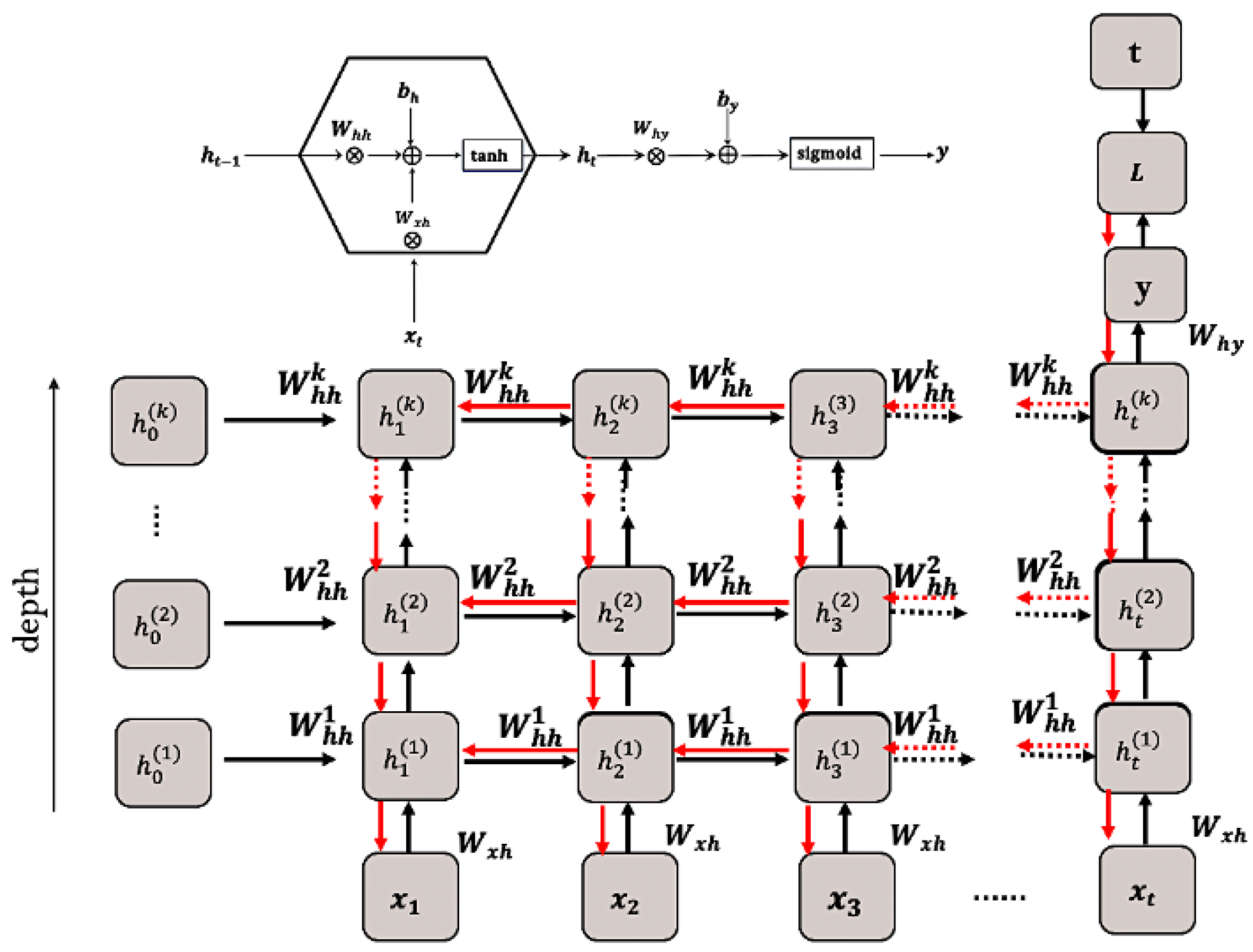
The Bees Algorithm was developed by Pham et al. with inspiration from clever foraging behaviours of the honey bees in nature [14]. In the proposed method the bee represents a sequential deep RNN model, which is modelled for the binary sentiment classification task. As can be seen in Figure 1, every bee (Sequential model) instance has the input layer, hidden deep RNN layers, and the output layer. The proposed model has the learnable parameters ${\theta =(W}_{xh},W_{hh},W_{hy},b_h,b_y)$, and aims to classify the sequential input data $(x_1,x_2,\dots {,x}_{t-1},x_t)$ to its targeted class t.

Based on the training procedure of the RNN model, each “bee model” has its own forward propagation action to calculate the initial solutions, local search procedure by gradient descent training with singular value decomposition (SVD), and global search actions to find the optimal parameters ${\theta =(W}_{xh},W_{hh},W_{hy},b_h,b_y)$ via the binary cross-entropy loss function (fitness function) $L_{BCE}(f(x^{\left(i\right)},\theta ),y^{\left(i\right)})$ as defined Section 3.3.

BA-3+ does not require a large population, which is a drawback with other population-based methods. BA-3+ employs only three individual bees for each training time. Each iteration begins with these three initial solutions as a forward pass of the model and continues with specified search strategies including exploitative local search, stochastic gradient descent (SGD) stabilised by Singular Value Decomposition (SVD), and explorative global search.

As with the basic Bees Algorithm [14], the initial candidate solutions are sorted. The maximum fitness value is selected as the best RNN bee for the local exploitative search. The worst fitness value (third bee) is selected for global search to avoid getting trapped at local optima, and the remaining RNN, i.e., the middle RNN bee is selected for stochastic gradient-descent learning with the stabilisation strategy of SVD operator to update weights and biases without vanishing and exploding gradients.

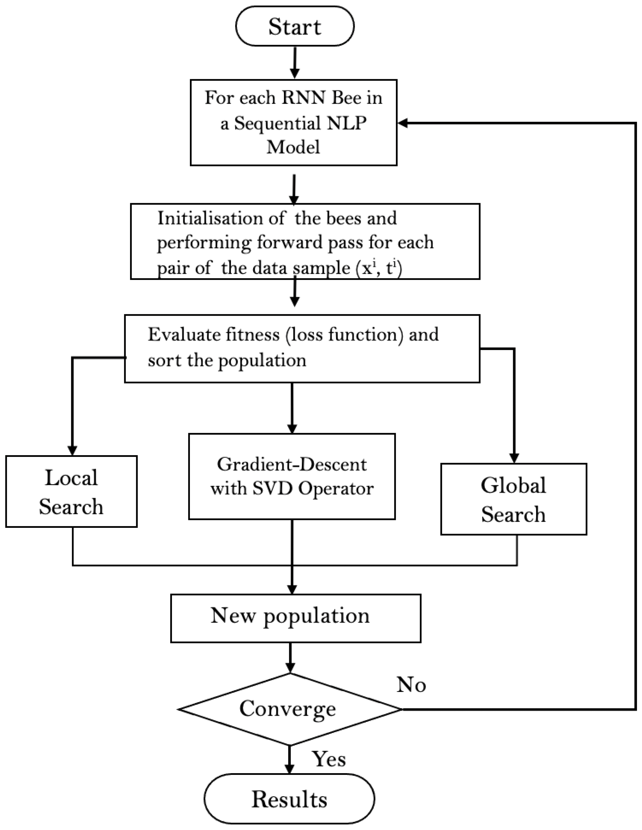
Figure 2 represents the flowchart of the proposed algorithm. ($x^{\left(train\right)},t^{\left(train\right)}$) is the training sample from the dataset, that $x^{\left(i\right)}=(x_1,x_2,\dots {,x}_{t-1},x_t)$ is defined as an n-dimensional sequential input and $t^{\left(i\right)}\in \left\{0,1\right\}$ is its targeted sentiment class. Parameters of the deep RNN model trained by using BA-3+ are shown in

Table 3. Parameters of the deep RNN model trained by using BA-3+.

Parameters	Information
$x^{\left(i\right)}=(x_1,x_2,\dots {,x}_{t-1},x_t)$	ith temporal sequential input from the input training set
$t^{\left(i\right)}$	ith targeted class of the output training set
$y^{\left(i\right)}$	ith predicted class of the $x^{\left(i\right)}$
$W_{xh}$	Weight matrix from input layer to hidden layer
$W_{hh}$	Weight matrix from hidden layer to hidden layer
$W_{hy}$	Weight matrix from hidden layer to output layer
$b_h,b_y$	Biases for the hidden layer and the output layer
nScout	Number of scout bees for initialisation
ngh	Neighbourhood size for the local search
nhidden	Hidden layer size
$\eta$	Learning rate for SGD

. Three initial solutions are calculated with the initial trainable parameters $\theta$ (see

Table 4. Learnable (trainable) parameters.

Parameters	Dimension
$W_{xh}$	${\mathbb{R}}^{number\mathit{of}\mathit{hidden}\mathit{layers}\times \mathit{dimension}\mathit{of}\mathit{each}\mathit{word}}$
$W_{hh}$	${\mathbb{R}}^{\mathit{number}\mathit{of}\mathit{hidden}\mathit{layers}\times \mathit{number}\mathit{of}\mathit{hidden}\mathit{layers}}$
$W_{hy}$	${\mathbb{R}}^{\left|\mathit{V}\right|\times \mathit{number}\mathit{of}\mathit{hidden}\mathit{layers}}$
$b_h$	${\mathbb{R}}^{\mathit{number}\mathit{of}\mathit{hidden}\mathit{layers}}$
$b_y$	${\mathbb{R}}^{\mathit{number}\mathit{of}\mathit{output}\mathit{layers}}$
$\left|\mathit{V}\right|:$	$\mathit{number}\mathit{of}\mathit{words}\mathit{in}\mathit{the}\mathit{vocabulary}$

) and sorted according to the loss function. The elite (best) RNN bee performs the local search operator, the middle RNN bee performs stochastic gradient-descent with SGD operator, and the third RNN bee performs global search. The optimisation continues with a new population of bees until the stopping criteria met; in other words, until the loss value is converged to zero.

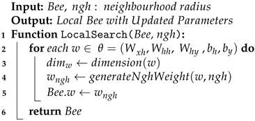
4.2. Local Search Operator

The local search procedure in the basic Bees Algorithm includes improving a promising solution within the neighbourhood of the selected solution parameters. In Algorithms 1 and 2, ngh represents the initial size of the neighbourhood for the local search. The neighbourhood begins as a large area and it is reduced by using a shrinking method [86] at each iteration according to the formula $ngh(t+1)=\alpha ngh\left(t\right)$. Here, $\alpha$ is usually a number between 0 and 1. The neighbourhood matrix is generated with the same dimension of each weight matrix of the learnable parameters ${\theta =(W}_{xh},W_{hh},W_{hy},b_h,b_y)$, and then is aded to the original weight matrix to obtain the updated weights. The pseudo-code to generate neighbourhood weights is given in Algorithm 2. The updated local weights are used for the local search of BA-3+ that can be seen in Algorithm 4.

Algorithm 1: Pseudo-code to generate neighbourhood weights.

Algorithm 2: Pseudo-code of the local search operator of BA-3+.

4.3. Enhanced Local Search by SGD and Singular Value Decomposition (SVD) Operator

As analysed in Section 3.2 and Section 3.3 due to the sharing the same hidden matrix $W_{hh}$ across the deep hidden layers and multiplying it again and again at every time step of the BPTT algorithm, the eigenvalues of the Jacobian matrix exponentially grow or vanish after t time steps. To handle this issue, it has been proposed to use a singular value decomposition of the hidden layer matrix to stabilise the eigenvalues of the updated matrix in the enhanced local search of BA-3+. As an example, assume that the eigenvalues of the $W_{hh}$ are represented ${\lambda }_1,{\lambda }_2,\dots ,{\lambda }_n$ The singular values of $W_{hh}$ can be founded by using the positive eigenvalues of the matrix $W_{hh}{W_{hh}}^T$, for every ${{\lambda }_i\ge 0\in \lambda }_1,{\lambda }_2,\dots ,{\lambda }_n,$ and $S_i=\sqrt{{\lambda }_i}$ if $W_{hh}$ is positive semi-definite square matrix [87]. Since the learnable parameters of the RNN can also be rectangular matrices, it is needed to find singular values of an arbitrary matrix A.

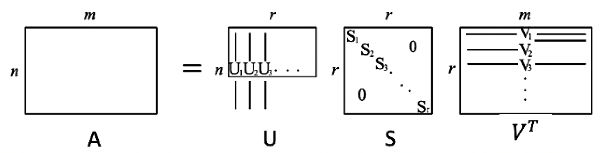
It is well-known that every arbitrary real matrix can be represented by the product of three matrices as $A=US{V}^T$, which is called singular value decomposition (SVD) of matrix A, which is used to find the singular values [88]. Figure 3 represents the SVD of an $n\times m$ dimensional matrix. Here, S is the $r\times r$ dimensional diagonal matrix $S_{n\times n}=diag[S_1,S_2,\dots ,...,S_n]$ that each $S_i$ represents the singular values of the matrix A, and U and V contain the corresponding singular vectors where U and V are orthogonal matrices with the $n\times r$ and $r\times m$ dimensions, respectively.

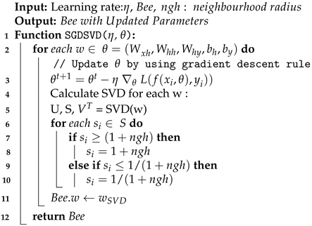
After updating each parameter of the ${\theta =(W}_{xh},W_{hh},W_{hy},b_h,b_y)$ by SGD rule, the SVD operator has used to control the eigenvalues of each parameter. The method aims to keep the singular values of the updated matrix close to 1 for gradient stabilisation. To this end, the SVD decomposition of the updated matrix is performed to find the singular values, and then every singular vector is controlled to be close to the unit vector. As given in Algorithm 3, the singular values of the updated weight matrix are restricted to the interval $[1/(1+ngh),1+ngh]$ to avoid updating in the wrong direction. Here, ngh is the initial neighbourhood size, which is chosen between $(0,1)$. As a result, $W_{hh}$ can be updated over time without vanishing or exploding gradients.

Algorithm 3: Pseudo-code of SGD with the SVD operator.

4.4. Global Search Operator

Besides the enhanced local search procedures, the proposed algorithm also includes a global search operator that combines random sampling chances which is also a good strategy for escaping local optimum points of the solution space. The third bee in a colony is used for the random exploration for potential new solutions of the search space. If the updated random weights gave a better solution for the loss function, then the third bee is updated with new global searched weights. This procedure gives the advantage to escape getting trapped at local optima, which results in converging to the global optimum faster during the training process. Algorithm 4 shows the pseudo-code of the proposed enhanced Ternary Bees Algorithm (BA-3+). The source code of the proposed algorithm is given at Appendix A.

Algorithm 4: Pseudo-code of the enhanced Ternary Bees Algorithm (BA-3+) for training deep RNN model.

In this study, sentiment analysis is considered as a binary classification problem. The F1-score or F1 measure was used as a statistical measure for the analysis of the binary classification problem in addition to the accuracy measure. F1 measure is calculated as follows:

$$\begin{array}{c}\hfill F_1=\frac{2PrecisionRecall}{Precision+Recall}\end{array}$$

(15)

$$\begin{array}{c}\hfill Precision=\frac{TP}{(TP+FP)}\end{array}$$

(16)

$$\begin{array}{c}\hfill Recall=\frac{TP}{(TP+FN)}\end{array}$$

(17)

$$\begin{array}{c}\hfill Accuracy=\frac{TP+TN}{(TP+TN+FP+FN)}\end{array}$$

(18)

Precision is the total count of true positives divided by the total number of positive results. The recall is the total number of true positive results divided by the number of all samples that should have been classified as positive. F1 measure can also be defined as a harmonic mean of the precision and recall value. The next section reports the details of the proposed algorithm’s experimental setup and performance results and benchmarks.

5. Results

5.1. Experimental Setup

The proposed algorithms were implemented using the Tensorflow library with Keras Sequential model in Python on the macOS Catalina on MacBook Pro, 3.1 GHz quad-core Intel Core i5 hardware. The proposed BA-3+ algorithm was run with batch size 1 for each $(x^{\left(i\right)}=(x_1,x_2,\dots {,x}_{t-1},x_t),t^{\left(i\right)})$ pair of datasets. Each dataset was divided into a training set ($\%80$ of the dataset) and a validation set ($\%20$ of the dataset) by using 5-fold cross-validation. The training was performed with BA-3+ and SGD according to BCE loss value over 100 independent runs, each involving 100 epochs. The BA-3+ training procedure was online learning and happened incrementally over each iteration, which means the learnable parameters were updated after each forward and backward propagation of each training sample [89]. Figure 4 represents the flowchart of the proposed classification model. The model implemented with Python Programming language with on Google Colab IDE [90] by using various tools and libraries, including TensorFlow [91], Keras [92], SciPy [93], NumPy [94], Pandas [95], and Matplotlib [96].

5.2. Parameter Tuning

Table 5. Parameter setting.

Parameter	Value
$x^{\left(i\right)}=(x_1,x_2,\dots {,x}_{t-1},x_t)$	max length = 200
nScout	3
nEiteSiteBee	1
nSelectedSiteBee	1
ngh	0.5
nhidden	32
epoch	100
independent runs (solution numbers)	100
batch size	1
upper limit of max singular value	$1+ngh$
lower limit of min singular value	$1/(1+ngh)$
$\eta$ (learning rate)	0.01

reports the parameters of BA-3+. The number of scout bees represents the number of sequential RNN networks. Each training sample of the input data $x^{\left(i\right)}=(x_1,x_2,\dots {,x}_{t-1},x_t)$ is padded to the maximum sequence length after pre-processing steps of the given dataset. Nine widely-used sentiment classification datasets in Turkish and English from three different domains (movie reviews, multi-domain product reviews, and Twitter reviews) were adopted to verify the proposed algorithm.

For each dataset, the sequential model was implemented with the same hyperparameters for the sake of fair comparison. Every sequential model was constructed with the input layer, hidden RNN layers, and the output layer. The embedding layer was used as the input layer, which converts the indexes of the sequential input to the fixed size dense vectors as an input of the model. The vocabulary size of each dataset was used as the input dimension of the embedding layer. The random uniform function was used as a weight initialiser for both the embedding layer and hidden layers.

As a critical hyper-parameter, the neighbourhood size (ngh) of the BA-3+ is set to 0.5. The learning rate $\left(\eta \right)$ of the SGD is set to 0.01. The neighbourhood size is used for both the local search and the stabilisation of the largest and the smallest eigenvalue of the updated parameters. The number of hidden layers is set to 32 for each model. Each element of the learnable (trainable) parameter of the ${\theta =(W}_{xh},W_{hh},W_{hy},b_h,b_y)$, the dimension of the weight matrices is changed according to hidden layer numbers, and the corresponding dimensions of the weight matrix can be seen in Table 4, in Section 4.2.

5.3. Results and Discussion

Table 6. Comparison of the results of 100 independent experiments with 100 epochs.

		Accuracy Results				Loss Results				F1 Score
Datasets	Alg.	${\mathit{Train}}_{\mathit{Best}}$	${\mathit{Val}}_{\mathit{Best}}$	${\mathit{Train}}_{\mathit{Avg}}$	${\mathit{Val}}_{\mathit{Avg}}$	${\mathit{Train}}_{\mathit{Best}}$	${\mathit{Val}}_{\mathit{Best}}$	${\mathit{Train}}_{\mathit{Avg}}$	${\mathit{Val}}_{\mathit{Avg}}$	${\mathit{Train}}_{\mathit{Avg}}$	${\mathit{Val}}_{\mathit{Avg}}$
TR Book	BA-3+	0.99	0.99	0.801	0.882	0.00	0.00	0.0769	0.117	0.81	0.78
	SGD	0.73	0.64	0.527	0.51	0.686	0.688	0.695	0.697	0.68	0.67
TR DVD	BA-3+	0.99	0.99	0.923	0.91	0.00	0.00	0.076	0.089	0.80	0.78
	SGD	0.52	0.39	0.519	0.389	0.686	0.701	0.708	0.748	0.70	0.70
TR Elect.	BA-3+	0.99	0.99	0.915	0.916	0.00	0.00	0.084	0.083	0.83	0.81
	SGD	0.99	0.58	0.615	0.549	0.092	0.684	0.640	0.849	0.75	0.73
TR Kitchen	BA-3+	0.99	0.99	0.81	0.810	0.00	0.00	0.189	0.191	0.81	0.75
	SGD	0.52	0.54	0.507	0.525	0.692	0.689	0.640	0.813	0.70	0.67
EN IMDB	BA-3+	0.99	0.99	0.911	0.90	0.00	0.00	0.032	0.006	0.77	0.75
	SGD	0.58	0.47	0.579	0.469	0.68	0.693	0.81	0.870	0.71	0.70
TR Twitter	BA-3+	0.99	0.99	0.914	0.830	0.00	0.00	0.017	0.029	0.76	0.73
	SGD	0.99	0.55	0.747	0.456	0.112	0.691	0.51	0.909	0.59	0.57
TR Movie	BA-3+	0.99	0.99	0.93	0.855	0.00	0.00	0.00	0.05	0.80	0.77
	SGD	0.9	0.58	0.58	0.494	0.376	0.689	0.668	0.725	0.66	0.63
EN Movie	BA-3+	0.99	0.99	0.896	0.87	0.00	0.00	0.024	0.058	0.81	0.80
	SGD	0.640	0.610	0.585	0.601	0.655	0.668	0.69	0.678	0.77	0.75
EN Yelp	BA-3+	0.99	0.99	0.87	0.86	0.00	0.00	0.030	0.02	0.75	0.70
	SGD	0.87	0.809	0.79	0.854	0.325	0.318	0.490	0.424	0.61	0.57

reports the best and average accuracy, loss, and F1 measures obtained by both the BA-3+ and SGD algorithms. The accuracy and loss values of the training and validation datasets are given as percentages. The average values were calculated after 100 independent training runs. Figure 5 shows the loss values for each dataset after one independent run which contains 100 training epochs. According to experimental results, the proposed BA-3+ algorithm guarantees fast convergence to the optimum value and the lowest error rate for each dataset. As can be clearly seen in Figure 6 and Figure 7, BA-3+ obtained the best solution within the first 20 iterations for each dataset. Besides, the gap between training and validation performance is small, which means BA-3+ prevents overfitting.

Figure 6 and Figure 7 represent the distributions of the loss values for both BA-3+ and SGD over 100 independent runs. Table 6 reports the best and average accuracy and loss values of the training datasets and validation datasets. BA-3+ performs better compared to traditional SGD. Results showed that BA-3+ can be used as an effective learning method for the sentiment classification task. The performances of BA-3+ were better both in terms of the best and average accuracy compared to SGD. Similarly, the best and average values of BA-3+ were lower than for SGD for each dataset.

BA-3+ has been compared with Differential Evolution (DE) and Particle Swarm Optimization (PSO) algorithms. For the sake of comparison, PSO has been evaluated with three particles as we propose to employ only three scout bees over 100 epochs. However, DE has been employed with 100 generations since it gave too low accuracy when it employees with only three generations.

Table 7. Total training time (sec) of the BA-3+, DE, PSO and SGD algorithms.

Datasets	SGD Total Time	BA3+ Total Time	DE Total Time	PSO Total Time
TR Book	237.36	393.139	871.608	544.914
TR DVD	233.92	407.187	860.439	520.700
TR Elect.	233.15	411.297	1317.971	512.482
TR Kitchen	235.73	417.765	855.125	513.929
TR Movie	1021.38	1394.631	3827.576	3969.091
TR Twitter	4334.98	8340.9	16,178.52	8978.6
EN IMDB	12,100.00	22,347.5	31,724.76	25,674.5
EN Movie	1293.718	2206.8	3361.95	2399.71
EN Yelp	4691.78	12,112.8	21,157.6	13,894.9

reports the time consumption of the SGD, BA-3+, DE, and PSO algorithms in second. As can be seen in

Table 8. Comparison of BA-3+ performance with DE and PSO and SGD.

Datasets	SGD Acc.	BA3+ Acc.	DE Acc.	PSO Acc.
TR Book	0.527	0.801	0.789	0.690
TR DVD	0.519	0.923	0.808	0.678
TR Elect.	0.58	0.915	0.786	0.696
TR Kitchen	0.507	0.81	0.794	0.686
TR Movie	0.58	0.93	0.887	0.759
TR Twitter	0.747	0.914	0.74	0.709
EN IMDB	0.579	0.91	0.778	0.701
EN Movie	0.585	0.896	0.78	0.69
EN Yelp	0.79	0.87	0.71	0.68

, BA-3+ has outperformed the DE and PSO, and its computation time of the BA-3+ is lower from DE and PSO. Although BA-3+ time consumption was longer than standard SGD, the accuracy value and F1 measure have improved for all classification datasets, at least with a 30–40% improvement. Furthermore, BA-3+ was more stable and converged faster than the DE and PSO algorithms since it employs only three individual bees as a population. As is expected SGD model has the lowest computation time, but the accuracy result is also lower compared to all other metaheuristic training algorithms.

Since we aim to improve the learning capacity of RNN as good as advanced deep learning language models such as LSTMs, we compared the proposed training algorithm with the advanced neural language models, including chain-structured and tree-structured language models. For this purpose, LSTM has been modeled with the same hidden layer number and training optimizer. Tree-LSTM has been modeled with similar hyperparameters to the RNTN model, which operates over MS-TR treebank [97]. The results of the Recursive Neural Tensor Network (RNTN) model have been taken from [97].

Table 9. Parameter setting for LSTM and Tree-LSTM models.

Parameter	Value
$x^{\left(i\right)}=(x_1,x_2,\dots {,x}_{t-1},x_t)$	max length = 50
embedding dimension	300
nhidden	32
epoch	100
batch size	32
optimizer	SGD
learning rate	0.01

reports the hyperparameters of the advanced deep language models and

Table 10. Comparisons of average accuracy results of advanced recurrent and recursive language models for Turkish binary classification datasets.

Models	Book	Electr.	DVD	Kitchen	Movie	Twitter
LSTM	0.823	0.725	0.751	0.75	0.835	0.895
Tree-LSTM	0.883	0.853	0.85	0.82	0.88	0.89
RNTN	0.86	0.866	0.824	0.798	0.88	0.835
RNN BA3+	0.88	0.801	0.866	0.818	0.854	0.838
RNN SGD	0.808	0.75	0.734	0.704	0.721	0.744

reports comparisons of accuracy results of advanced recurrent and recursive language models for Turkish binary classification datasets over test dataset. According to the experiments, it is observed that the RNN model combined with the BA-3+ training algorithm performed close or as good as advanced recurrent and recursive deep language models and gave comparable results.

As it can be clearly seen from Figure 8, RNN-SGD performed well for only one dataset. Accordingly, we can say that the performance of the systems can be better when the models are trained with huge datasets such as the Twitter classification dataset (see Table 2). However, in all other cases, we found that the BA algorithm performed well and yielding results just as well as advanced language models. The experimental results demonstrate that BA-3+ gives us a chance to get rid of the disadvantages of the SGD algorithm and can handle the VEG problem. Although BA-3+ time consumption is longer than SGD, the accuracy value and F1 measure are higher for all classification datasets. Furthermore, since BA-3+ employs only three scout bees, the total training time is shorter than the DE and PSO algorithms and it outperformed the DE and PSO (see Table 7 and Table 8). BA-3+ and PSO runtimes are similar, but BA-3+ gave better results in terms of accuracy. Even though the DE algorithm was tested for 100 generations, it could not reach the BA-3+ performance.

The success of BA-3+ depends on its hybrid metaheuristic nature. BA-3+ evaluates only three candidate models, each having the same deep RNN architecture with different learnable parameters. The training process starts with these three candidate models (number of scout bees), which dynamically search for the optimum values of the learnable parameters, and continues selecting the best model for local search to find better solutions. This is the feature of BA-3+ that brings good initial parameters for the iterative learning process. After each iteration of the proposed algorithm, if more optimum values of the learnable parameters are found, they will be updated incrementally. This feature of BA-3+ yields faster convergence. Additionally, as BA-3+ combines local SGD training with the SVD, it can exploit the learning ability of SGD while controlling vanishing and exploding gradients, making BA-3+ a hybrid meta-learning algorithm combining gradient-free and gradient-based optimisation. Finally, BA-3+ has a random exploration operator, namely, a global search operator, which enables the exploration of new promising solutions while preventing the optimisation process from being trapped at local stationary points. Besides these advantages, critical hyperparameters, such as learning rate and neighbourhood size, were empirically selected for BA-3+ as for SGD.

In the future, the proposed algorithm will be compared to the recent metaheuristic methods, such as advanced backtracking search optimisation algorithm (ABSA) [77], which has proved its performance superiority compared to the GA, DE, and backtracking search optimization algorithm (BSA) for global optimisation [76]. Since we recommend using only three individual bees as population size, we think it would be unfair to compare BA-3+ with all other population-based metaheuristic algorithms using higher population sizes without any SGD-SVD local search. Therefore, the previous population-based metaheuristics should be improved with hybrid approaches to work well with lower population sizes in the future. Furthermore, the hyperparameter tuning study will be done since the deep learning model and metaheuristic algorithms are sensible to critical hyperparameters. The proposed algorithm will also be tested for fine-grained classification problems with more than two classes. Although the accuracy rate of the proposed algorithm is high, strategies should be found to ensure faster convergence in terms of time. Learning large datasets may also require the parallel running of the proposed algorithm and more powerful hardware resources.

6. Conclusions

This paper has described the use of the Ternary Bees Algorithm (BA-3+) as a training algorithm for finding the optimal set of parameters of a sequential deep RNN language model for the sentiment classification task. BA-3+ has been modeled as a sequential model and tested on nine different datasets including Turkish and English text. The model conducts an exploitative local search with the best bee and an explorative global search with the worst bee. The in-between bee is used for improved Stochastic Gradient Descent (SGD) learning with Singular Value Decomposition (SVD) to stabilise the updated model parameters after the application of SGD. This strategy is adopted to prevent the vanishing and exploding gradients problem of SGD training. The proposed BA-3+ algorithm guarantees fast convergence as it combines local search, global search, and SGD learning with SVD, and it is faster than other iterative, metaheuristic algorithms, as it employs only three candidate solutions in each training step. BA-3+ has been tested on the sentiment classification task with different datasets, and comparative results were obtained for chain-structured and tree-structured deep language models, Differential Evolution (DE), and Particle Swarm Optimization (PSO) algorithms. BA-3+ converged to the global minimum faster compared to the DE and PSO algorithms and it outperformed the SGD, DE, and PSO algorithms both for the Turkish and English datasets. According to the experimental results, BA-3+ performed better compared to the standard SGD training algorithm and RNN combined with BA-3+ performs as good as for advanced deep neural language models. The small differences between the training and validation results for the nine datasets have confirmed the efficiency of the proposed algorithm, with BA-3+ indeed offering better generalisation and faster convergence than the SGD algorithm.

References

1. Mikolov, T.; Karafiát, M.; Burget, L.; Jan, C.; Khudanpur, S. Recurrent neural network based language model. In Proceedings of the 11th Annual Conference of the International Speech Communication Association, Interspeech 2010, Makuhari, Japan, 26–30 September 2010; pp. 1045–1048. [Google Scholar]
2. Che, Z.; Purushotham, S.; Cho, K.; Sontag, D.; Liu, Y. Recurrent Neural Networks for Multivariate Time Series with Missing Values. Sci. Rep. 2018, 8. [Google Scholar] [CrossRef] [Green Version]
3. Kalchbrenner, N.; Blunsom, P. Recurrent Continuous Translation Models. In Proceedings of the 2013 Conference on Empirical Methods in Natural Language Processing, Association for Computational Linguistics, Seattle, WA, USA, 18–21 October 2013; pp. 1700–1709. [Google Scholar]
4. You, Q.; Jin, H.; Wang, Z.; Fang, C.; Luo, J. Image captioning with semantic attention. In Proceedings of the IEEE Computer Society Conference on Computer Vision and Pattern Recognition, Las Vegas, NV, USA, 27–30 June 2016. [Google Scholar] [CrossRef] [Green Version]
5. Pascanu, R.; Mikolov, T.; Bengio, Y. On the Difficulty of Training Recurrent Neural Networks. In Proceedings of the 30th International Conference on International Conference on Machine Learning-Volume 28, JMLR.org (ICML’13), Atlanta, GA, USA, 16–21 June 2013; pp. III-1310–III-1318. [Google Scholar]
6. Lecun, Y.; Bengio, Y.; Hinton, G. Deep Learning; MIT Press: Cambridge, MA, USA, 2015. [Google Scholar] [CrossRef]
7. Bengio, Y.; Simard, P.; Frasconi, P. Learning Long-Term Dependencies with Gradient Descent is Difficult. IEEE Trans. Neural Netw. 1994. [Google Scholar] [CrossRef] [PubMed]
8. Hochreiter, S.; Schmidhuber, J. Long Short-Term Memory. Neural Comput. 1997. [Google Scholar] [CrossRef] [PubMed]
9. Chung, J.; Gulcehre, C.; Cho, K.; Bengio, Y. Gated Feedback Recurrent Neural Networks. In Proceedings of the 32nd International Conference on Machine Learning-Volume 37. JMLR.org (ICML’15), Lille, France, 6–11 July 2015; pp. 2067–2075. [Google Scholar]
10. Sutskever, I.; Hinton, G. Learning multilevel distributed representations for high-dimensional sequences. J. Mach. Learn. Res. 2007, 2, 548–555. [Google Scholar]
11. Sutskever, I. Training Recurrent Neural Networks. Ph.D. Thesis, University of Toronto, Toronto, ON, Canada, 2013. [Google Scholar]
12. Srivastava, N.; Hinton, G.; Krizhevsky, A.; Sutskever, I.; Salakhutdinov, R. Dropout: A simple way to prevent neural networks from overfitting. J. Mach. Learn. Res. 2014, 15, 1929–1958. [Google Scholar]
13. Darwish, A.; Hassanien, A.E.; Das, S. A survey of swarm and evolutionary computing approaches for deep learning. Artif. Intell. Rev. 2020. [Google Scholar] [CrossRef]
14. Pham, D.T.; Ghanbarzadeh, A.; Koç, E.; Otri, S.; Rahim, S.; Zaidi, M. The Bees Algorithm-A Novel Tool for Complex Optimisation Problems. In Proceedings of the Intelligent Production Machines and Systems-2nd I*PROMS Virtual International Conference, Online, 3–14 July 2006. [Google Scholar] [CrossRef]
15. Pham, D.T.; Koç, E.; Ghanbarzadeh, A. Optimization of the Weights of Multi-Layered Perceptions Using the Bees Algorithm. In Proceedings of the International Symposium on Intelligent Manufacturing Systems, Online, 3–14 July 2006; Volume 5, pp. 38–46. [Google Scholar]
16. Ismail, A.H.; Hartono, N.; Zeybek, S.; Pham, D.T. Using the Bees Algorithm to solve combinatorial optimisation problems for TSPLIB. In Proceedings of the IOP Conference Series: Materials Science and Engineering, Batu, Indonesia, 17–19 March 2020; Volume 847. [Google Scholar] [CrossRef]
17. Laili, Y.; Tao, F.; Pham, D.T.; Wang, Y.; Zhang, L. Robotic disassembly re-planning using a two-pointer detection strategy and a super-fast bees algorithm. Robot. Comput. Integr. Manuf. 2019. [Google Scholar] [CrossRef]
18. Jaeger, H.; Haas, H. Harnessing Nonlinearity: Predicting Chaotic Systems and Saving Energy in Wireless Communication. Science 2004. [Google Scholar] [CrossRef] [Green Version]
19. Greff, K.; Srivastava, R.K.; Koutnik, J.; Steunebrink, B.R.; Schmidhuber, J. LSTM: A Search Space Odyssey. IEEE Trans. Neural Netw. Learn. Syst. 2017. [Google Scholar] [CrossRef] [Green Version]
20. Martens, J.; Sutskever, I. Learning recurrent neural networks with Hessian-free optimization. In Proceedings of the 28th International Conference on Machine Learning (ICML 2011), Bellevue, WA, USA, 28 June–2 July 2011. [Google Scholar]
21. Yang, S.; Chen, D.; Li, S.; Wang, W. Carbon price forecasting based on modified ensemble empirical mode decomposition and long short-term memory optimized by improved whale optimization algorithm. Sci. Total Environ. 2020, 716, 137117. [Google Scholar] [CrossRef] [PubMed]
22. Peng, L.; Zhu, Q.; Lv, S.X.; Wang, L. Effective long short-term memory with fruit fly optimization algorithm for time series forecasting. Soft Comput. 2020, 24, 15059–15079. [Google Scholar] [CrossRef]
23. ElSaid, A.E.R.; El Jamiy, F.; Higgins, J.; Wild, B.; Desell, T. Optimizing long short-term memory recurrent neural networks using ant colony optimization to predict turbine engine vibration. Appl. Soft Comput. J. 2018. [Google Scholar] [CrossRef] [Green Version]
24. Rashid, T.A.; Fattah, P.; Awla, D.K. Using Accuracy Measure for Improving the Training of LSTM with Metaheuristic Algorithms. Procedia Comput. Sci. 2018, 140, 324–333. [Google Scholar] [CrossRef]
25. Srivastava, R.K.; Greff, K.; Schmidhuber, J. Training Very Deep Networks. In Proceedings of the 28th International Conference on Neural Information Processing Systems-Volume 2 (NIPS’15), Montreal, QC, Canada, 7–12 December 2015; MIT Press: Cambridge, MA, USA, 2015; pp. 2377–2385. [Google Scholar]
26. Somu, N.; M R, G.R.; Ramamritham, K. A hybrid model for building energy consumption forecasting using long short term memory networks. Appl. Energy 2020, 261, 114131. [Google Scholar] [CrossRef]
27. Bouktif, S.; Fiaz, A.; Ouni, A.; Serhani, M.A. Multi-Sequence LSTM-RNN Deep Learning and Metaheuristics for Electric Load Forecasting. Energies 2020, 13, 391. [Google Scholar] [CrossRef] [Green Version]
28. Nair, V.; Hinton, G.E. Rectified linear units improve Restricted Boltzmann machines. In Proceedings of the ICML 2010-Proceedings, 27th International Conference on Machine Learning, Haifa, Israel, 21–24 June 2010. [Google Scholar]
29. Glorot, X.; Bordes, A.; Bengio, Y. Deep sparse rectifier neural networks. J. Mach. Learn. Res. 2011, 15, 315–323. [Google Scholar]
30. Glorot, X.; Bengio, Y. Understanding the difficulty of training deep feedforward neural networks. J. Mach. Learn. Res. 2010, 9, 249–256. [Google Scholar]
31. Clevert, D.A.; Unterthiner, T.; Hochreiter, S. Fast and accurate deep network learning by exponential linear units (ELUs). In Proceedings of the 4th International Conference on Learning Representations, ICLR 2016-Conference Track Proceedings, San Juan, PR, USA, 2–4 May 2016. [Google Scholar]
32. Bengio, Y.; Boulanger-Lewandowski, N.; Pascanu, R. Advances in optimizing recurrent networks. In Proceedings of the 2013 IEEE International Conference on Acoustics, Speech and Signal Processing, Vancouver, BC, Canada, 26–31 May 2013; pp. 8624–8628. [Google Scholar] [CrossRef] [Green Version]
33. Le, Q.V.; Jaitly, N.; Hinton, G.E. A Simple Way to Initialize Recurrent Networks of Rectified Linear Units. arXiv 2015, arXiv:1504.00941. [Google Scholar]
34. Xu, X.; Ge, H.; Li, S. An improvement on recurrent neural network by combining convolution neural network and a simple initialization of the weights. In Proceedings of the 2016 the IEEE International Conference of Online Analysis and Computing Science (ICOACS 2016), Chongqing, China, 28–29 May 2016. [Google Scholar] [CrossRef]
35. Vorontsov, E.; Trabelsi, C.; Kadoury, S.; Pal, C. On orthogonality and learning recurrent networks with long term dependencies. In Proceedings of the 34th International Conference on Machine Learning (ICML 2017), Sydney, Australia, 6–11 August 2017. [Google Scholar]
36. Zhang, J.; Lei, Q.; Dhillon, I. Stabilizing Gradients for Deep Neural Networks via Efficient SVD Parameterization. In Proceedings of the 35th International Conference on Machine Learning (PMLR), Stockholm, Sweden, 10–15 July 2018; Dy, J., Krause, A., Eds.; Volume 80, pp. 5806–5814. [Google Scholar]
37. Becker, S.; le Cun, Y. Improving the Convergence of Back-Propagation Learning with Second Order Methods. In Proceedings of the 1988 Connectionist Models Summer School, San Francisco, CA, USA, 17–26 June 1989; pp. 29–37. [Google Scholar]
38. Kag, A.; Saligrama, V. Training Recurrent Neural Networks via Forward Propagation Through Time. In Proceedings of the 38th International Conference on Machine Learning (PMLR), Virtual, Online, 18–24 July 2021; Volume 139, pp. 5189–5200. [Google Scholar]
39. Yang, X.S. Nature-Inspired Metaheuristic Algorithms; Luniver Press: London, UK, 2008; ISBN 1905986106. [Google Scholar]
40. Chiroma, H.; Gital, A.Y.; Rana, N.; Abdulhamid, S.M.; Muhammad, A.N.; Umar, A.Y.; Abubakar, A.I. Nature Inspired Meta-heuristic Algorithms for Deep Learning: Recent Progress and Novel Perspective. Adv. Intell. Syst. Comput. 2020, 943, 59–70. [Google Scholar] [CrossRef]
41. Chong, H.Y.; Yap, H.J.; Tan, S.C.; Yap, K.S.; Wong, S.Y. Advances of metaheuristic algorithms in training neural networks for industrial applications. Soft Comput. 2021. [Google Scholar] [CrossRef]
42. Ouaarab, A.; Osaba, E.; Bouziane, M.; Bencharef, O. Review of Swarm Intelligence for Improving Time Series Forecasting. In Applied Optimization and Swarm Intelligence; Osaba, E., Yang, X.S., Eds.; Springer: Singapore, 2021; pp. 61–79. [Google Scholar] [CrossRef]
43. Muñoz-Ordóñez, J.; Cobos, C.; Mendoza, M.; Herrera-Viedma, E.; Herrera, F.; Tabik, S. Framework for the Training of Deep Neural Networks in TensorFlow Using Metaheuristics. In Intelligent Data Engineering and Automated Learning–IDEAL 2018; Yin, H., Camacho, D., Novais, P., Tallón-Ballesteros, A.J., Eds.; Springer International Publishing: Cham, Switzerland, 2018; pp. 801–811. [Google Scholar]
44. Ibrahim, A.M.; El-Amary, N.H. Particle Swarm Optimization trained recurrent neural network for voltage instability prediction. J. Electr. Syst. Inf. Technol. 2018, 5, 216–228. [Google Scholar] [CrossRef]
45. Duchanoy, C.A.; Moreno-Armendáriz, M.A.; Urbina, L.; Cruz-Villar, C.A.; Calvo, H.; Rubio, J.D.J. A novel recurrent neural network soft sensor via a differential evolution training algorithm for the tire contact patch. Neurocomputing 2017, 235, 71–82. [Google Scholar] [CrossRef]
46. Desell, T.; Clachar, S.; Higgins, J.; Wild, B. Evolving deep recurrent neural networks using ant colony optimization. In European Conference on Evolutionary Computation in Combinatorial Optimization; Lecture Notes in Computer Science (Including Subseries Lecture Notes in Artificial Intelligence and Lecture Notes in Bioinformatics); Springer International Publishing: Cham, Switzerland, 2015; Volume 9026, pp. 86–98. [Google Scholar] [CrossRef]
47. Juang, C.F. A Hybrid of Genetic Algorithm and Particle Swarm Optimization for Recurrent Network Design. IEEE Trans. Syst. Man Cybern. Part Cybern. 2004. [Google Scholar] [CrossRef]
48. Stanley, K.O.; Miikkulainen, R. Evolving neural networks through augmenting topologies. Evol. Comput. 2002. [Google Scholar] [CrossRef]
49. Ororbia, A.; ElSaid, A.E.R.; Desell, T. Investigating recurrent neural network memory structures using neuro-evolution. In Proceedings of the GECCO 2019-Proceedings of the 2019 Genetic and Evolutionary Computation Conference, Prague, Czech Republic, 13–17 July 2019; pp. 446–455. [Google Scholar] [CrossRef] [Green Version]
50. Wang, H.; Wang, H.; Xu, K. Evolutionary recurrent neural network for image captioning. Neurocomputing 2020, 401, 249–256. [Google Scholar] [CrossRef]
51. Camero, A.; Toutouh, J.; Alba, E. Random error sampling-based recurrent neural network architecture optimization. Eng. Appl. Artif. Intell. 2020, 96, 103946. [Google Scholar] [CrossRef]
52. Mo, H.; Custode, L.L.; Iacca, G. Evolutionary neural architecture search for remaining useful life prediction. Appl. Soft Comput. 2021, 108, 107474. [Google Scholar] [CrossRef]
53. Kang, Q.; Liao, W.K.; Agrawal, A.; Choudhary, A. A hybrid training algorithm for recurrent neural network using particle swarm optimization-based preprocessing and temporal error aggregation. In Proceedings of the IEEE International Conference on Data Mining Workshops, ICDMW, New Orleans, LA, USA, 18–21 November 2017. [Google Scholar] [CrossRef]
54. Eberhart, R.; Kennedy, J. New optimizer using particle swarm theory. In Proceedings of the International Symposium on Micro Machine and Human Science, Nagoya, Japan, 4–6 October 1995. [Google Scholar] [CrossRef]
55. Ge, H.W.; Liang, Y.C.; Marchese, M. A modified particle swarm optimization-based dynamic recurrent neural network for identifying and controlling nonlinear systems. Comput. Struct. 2007. [Google Scholar] [CrossRef]
56. Xiao, P.; Venayagamoorthy, G.K.; Corzine, K.A. Combined training of recurrent neural networks with particle swarm optimization and backpropagation algorithms for impedance identification. In Proceedings of the 2007 IEEE Swarm Intelligence Symposium (SIS 2007), Honolulu, HI, USA, 1–5 April 2007. [Google Scholar] [CrossRef]
57. Zhang, N.; Behera, P.K.; Williams, C. Solar radiation prediction based on particle swarm optimization and evolutionary algorithm using recurrent neural networks. In Proceedings of the SysCon 2013-7th Annual IEEE International Systems Conference, Proceedings, Orlando, FL, USA, 15–18 April 2013. [Google Scholar] [CrossRef]
58. Cai, X.; Zhang, N.; Venayagamoorthy, G.K.; Wunsch, D.C. Time series prediction with recurrent neural networks trained by a hybrid PSO-EA algorithm. Neurocomputing 2007. [Google Scholar] [CrossRef]
59. Blanco, A.; Delgado, M.; Pegalajar, M.C. A real-coded genetic algorithm for training recurrent neural networks. Neural Netw. 2001. [Google Scholar] [CrossRef] [Green Version]
60. Nawi, N.M.; Khan, A.; Rehman, M.Z.; Chiroma, H.; Herawan, T. Weight Optimization in Recurrent Neural Networks with Hybrid Metaheuristic Cuckoo Search Techniques for Data Classification. Math. Probl. Eng. 2015, 2015, 868375. [Google Scholar] [CrossRef] [Green Version]
61. Chuangxin, G.; Gen, Y.; Chengzhi, Z.; Xueping, W.; Xiu, C. SoC estimation for lithium-ion battery using recurrent NARX neural network and genetic algorithm. In Proceedings of the IOP Conference Series: Materials Science and Engineering, Hangzhou, China, 28–31 March 2019. [Google Scholar] [CrossRef]
62. Bas, E.; Egrioglu, E.; Kolemen, E. Training simple recurrent deep artificial neural network for forecasting using particle swarm optimization. Granul. Comput. 2021. [Google Scholar] [CrossRef]
63. Kaya, E.; Baştemur Kaya, C. A Novel Neural Network Training Algorithm for the Identification of Nonlinear Static Systems: Artificial Bee Colony Algorithm Based on Effective Scout Bee Stage. Symmetry 2021, 13, 419. [Google Scholar] [CrossRef]
64. Shettigar, A.K.; Patel, G.C.M.; Chate, G.R.; Vundavilli, P.R.; Parappagoudar, M.B. Artificial bee colony, genetic, back propagation and recurrent neural networks for developing intelligent system of turning process. SN Appl. Sci. 2020, 2, 660. [Google Scholar] [CrossRef] [Green Version]
65. Shishira, S.R.; Kandasamy, A. BeeM-NN: An efficient workload optimization using Bee Mutation Neural Network in federated cloud environment. J. Ambient Intell. Humaniz. Comput. 2021, 12, 3151–3167. [Google Scholar] [CrossRef]
66. Ruiz, L.G.B.; Capel, M.I.; Pegalajar, M.C. Parallel memetic algorithm for training recurrent neural networks for the energy efficiency problem. Appl. Soft Comput. 2019, 76, 356–368. [Google Scholar] [CrossRef]
67. Hu, H.; Wang, H.; Bai, Y.; Liu, M. Determination of endometrial carcinoma with gene expression based on optimized Elman neural network. Appl. Math. Comput. 2019, 341, 204–214. [Google Scholar] [CrossRef]
68. Tian, Y.; Peng, S.; Zhang, X.; Rodemann, T.; Tan, K.C.; Jin, Y. A Recommender System for Metaheuristic Algorithms for Continuous Optimization Based on Deep Recurrent Neural Networks. IEEE Trans. Artif. Intell. 2020, 1, 5–18. [Google Scholar] [CrossRef]
69. Roy, K.; Mandal, K.K.; Mandal, A.C. Ant-Lion Optimizer algorithm and recurrent neural network for energy management of micro grid connected system. Energy 2019, 167, 402–416. [Google Scholar] [CrossRef]
70. Ab Aziz, M.F.; Mostafa, S.A.; Mohd Foozy, C.F.; Mohammed, M.A.; Elhoseny, M.; Abualkishik, A.Z. Integrating Elman recurrent neural network with particle swarm optimization algorithms for an improved hybrid training of multidisciplinary datasets. Expert Syst. Appl. 2021, 183, 115441. [Google Scholar] [CrossRef]
71. Hassib, E.M.; El-Desouky, A.I.; Labib, L.M.; El-kenawy, E.S.M. WOA + BRNN: An imbalanced big data classification framework using Whale optimization and deep neural network. Soft Comput. 2020, 24, 5573–5592. [Google Scholar] [CrossRef]
72. Shah, H.; Chiroma, H.; Herawan, T.; Ghazali, R.; Tairan, N. An Efficient Bio-inspired Bees Colony for Breast Cancer Prediction. In Proceedings of the International Conference on Data Engineering 2015 (DaEng-2015); Abawajy, J.H., Othman, M., Ghazali, R., Deris, M.M., Mahdin, H., Herawan, T., Eds.; Springer: Singapore, 2019; pp. 597–608. [Google Scholar]
73. Kumar, K.; Haider, M.T.U. Enhanced Prediction of Intra-day Stock Market Using Metaheuristic Optimization on RNN–LSTM Network. New Gener. Comput. 2021, 39, 231–272. [Google Scholar] [CrossRef]
74. Martinez, A.D.; Del Ser, J.; Villar-Rodriguez, E.; Osaba, E.; Poyatos, J.; Tabik, S.; Molina, D.; Herrera, F. Lights and shadows in Evolutionary Deep Learning: Taxonomy, critical methodological analysis, cases of study, learned lessons, recommendations and challenges. Inf. Fusion 2021, 67, 161–194. [Google Scholar] [CrossRef]
75. Wolpert, D.H.; Macready, W.G. No Free Lunch Theorems for Optimization. Trans. Evol. Comp 1997, 1, 67–82. [Google Scholar] [CrossRef] [Green Version]
76. Zhang, Y. Backtracking search algorithm with specular reflection learning for global optimization. Knowl. Based Syst. 2021, 212, 106546. [Google Scholar] [CrossRef]
77. Wang, L.; Peng, L.; Wang, S.; Liu, S. Advanced backtracking search optimization algorithm for a new joint replenishment problem under trade credit with grouping constraint. Appl. Soft Comput. 2020, 86, 105953. [Google Scholar] [CrossRef]
78. Rumelhart, D.E.; Hinton, G.E.; Williams, R.J. Learning Internal Representations by Error Propagation. In Readings in Cognitive Science: A Perspective from Psychology and Artificial Intelligence; Elsevier: Amsterdam, The Netherlands, 2013. [Google Scholar] [CrossRef]
79. Demirtas, E.; Pechenizkiy, M. Cross-lingual polarity detection with machine translation. In Proceedings of the 2nd International Workshop on Issues of Sentiment Discovery and Opinion Mining, WISDOM 2013-Held in Conjunction with SIGKDD 2013, Chicago, IL, USA, 11 August 2013. [Google Scholar] [CrossRef]
80. Hayran, A.; Sert, M. Kelime Gömme ve Füzyon Tekniklerine Dayali Mikroblog Verileri Üzerinde Duygu Analizi. In Proceedings of the 2017 25th Signal Processing and Communications Applications Conference (SIU 2017), Antalya, Turkey, 15–18 May 2017. [Google Scholar] [CrossRef]
81. Maas, A.L.; Daly, R.E.; Pham, P.T.; Huang, D.; Ng, A.Y.; Potts, C. Learning Word Vectors for Sentiment Analysis. In Proceedings of the 49th Annual Meeting of the Association for Computational Linguistics: Human Language Technologies; Association for Computational Linguistics: Portland, OR, USA, 2011; pp. 142–150. [Google Scholar]
82. Pang, B.; Lee, L.; Vaithyanathan, S. Thumbs up? Sentiment Classification using Machine Learning Techniques. arXiv 2002, arXiv:cs/0205070. [Google Scholar]
83. Asghar, N. Yelp Dataset Challenge: Review Rating Prediction. arXiv 2016, arXiv:1605.05362. [Google Scholar]
84. Erhan, D.; Manzagol, P.A.; Bengio, Y.; Bengio, S.; Vincent, P. The Difficulty of Training Deep Architectures and the Effect of Unsupervised Pre-Training. In Proceedings of the Twelth International Conference on Artificial Intelligence and Statistics, Clearwater, FL, USA, 16–19 April 2009; van Dyk, D., Welling, M., Eds.; PMLR, Hilton Clearwater Beach Resort: Clearwater Beach, FL, USA, 2009; Volume 5, pp. 153–160. [Google Scholar]
85. Talathi, S.S.; Vartak, A. Improving Performance of Recurrent Neural Network with Relu Nonlinearity. arXiv 2015, arXiv:1511.03771. [Google Scholar]
86. Pham, D.T.; Castellani, M. A comparative study of the Bees Algorithm as a tool for function optimisation. Cogent Eng. 2015. [Google Scholar] [CrossRef]
87. Burden, R.L.; Faires, J.D. Numerical Analysis, 9th ed.; Brooks/Cole, Cengage Learning: Boston, MA, USA, 2011. [Google Scholar] [CrossRef]
88. Trefethen, L.N.; Bau, D. Numerical Linear Algebra; SIAM: Philadelphia, PA, USA, 1997. [Google Scholar] [CrossRef]
89. Bottou, L. On-line Learning and Stochastic Approximations. In On-Line Learning in Neural Networks; Saad, D., Ed.; Publications of the Newton Institute, Cambridge University Press: Cambridge, UK, 1999; pp. 9–42. [Google Scholar] [CrossRef] [Green Version]
90. Bisong, E. Google Colaboratory. In Building Machine Learning and Deep Learning Models on Google Cloud Platform: A Comprehensive Guide for Beginners; Apress: Berkeley, CA, USA, 2019; pp. 59–64. [Google Scholar] [CrossRef]
91. Abadi, M.; Agarwal, A.; Barham, P.; Brevdo, E.; Chen, Z.; Citro, C.; Corrado, G.S.; Davis, A.; Dean, J.; Devin, M.; et al. TensorFlow: Large-Scale Machine Learning on Heterogeneous Systems. 2015. Available online: https://www.tensorflow.org (accessed on 24 July 2021).
92. Chollet, F. Keras. 2015. Available online: https://github.com/fchollet/keras (accessed on 24 July 2021).
93. Virtanen, P.; Gommers, R.; Oliphant, T.E.; Haberland, M.; Reddy, T.; Cournapeau, D.; Burovski, E.; Peterson, P.; Weckesser, W.; Bright, J.; et al. SciPy 1.0: Fundamental Algorithms for Scientific Computing in Python. Nat. Methods 2020, 17, 261–272. [Google Scholar] [CrossRef] [Green Version]
94. Harris, C.R.; Millman, K.J.; van der Walt, S.J.; Gommers, R.; Virtanen, P.; Cournapeau, D.; Wieser, E.; Taylor, J.; Berg, S.; Smith, N.J.; et al. Array programming with NumPy. Nature 2020, 585, 357–362. [Google Scholar] [CrossRef] [PubMed]
95. McKinney, W. Data Structures for Statistical Computing in Python. In Proceedings of the 9th Python in Science Conference, Austin, TX, USA, 28 June–3 July 2010; pp. 51–56. [Google Scholar]
96. Hunter, J.D. Matplotlib: A 2D graphics environment. Comput. Sci. Eng. 2007, 9, 90–95. [Google Scholar] [CrossRef]
97. Zeybek, S.; Koc, E.; Seçer, A. MS-TR: A Morphologically Enriched Sentiment Treebank and Recursive Deep Models for Compositional Semantics in Turkish. Cogent Eng. 2021. [Google Scholar] [CrossRef]
Figure 1. A Deep RNN architecture representing a bee in the proposed algorithm. Black lines are the forward pass of RNN cell at time t (unfolded version at upper) and red lines representing the error backpropagation through long-term dependencies.
Symmetry 13 01347 g001
Figure 2. Flowchart of the proposed enhanced Ternary Bees Algorithm (BA-3+).
Symmetry 13 01347 g002
Figure 3. Singular Value Decomposition (SVD) of matrix A.
Symmetry 13 01347 g003
Figure 4. Flowchart of the proposed classification model.
Symmetry 13 01347 g004
Figure 5. Comparison of the loss values of BA-3+ (TBA) and SGD for one independent run.
Symmetry 13 01347 g005
Figure 6. Distributions of the loss values of the training and validation dataset for 100 independent runs.
Symmetry 13 01347 g006
Figure 7. Distributions of the loss values of the training and validation dataset for 100 independent runs.
Symmetry 13 01347 g007
Figure 8. Comparison of BA-3+ performance with advanced models and RNN model trained with SGD for some datasets.
Symmetry 13 01347 g008