The Skewed-Elliptical Log-Linear Birnbaum–Saunders Alpha-Power Model

Abstract

In this paper, the skew-elliptical sinh-alpha-power distribution is developed as a natural follow-up to the skew-elliptical log-linear Birnbaum–Saunders alpha-power distribution, previously studied in the literature. Special cases include the ordinary log-linear Birnbaum–Saunders and skewed log-linear Birnbaum–Saunders distributions. As shown, it is able to surpass the ordinary sinh-normal models when fitting data sets with high (above the expected with the sinh-normal) degrees of asymmetry. Maximum likelihood estimation is developed with the inverse of the observed information matrix used for standard error estimation. Large sample properties of the maximum likelihood estimators such as consistency and asymptotic normality are established. An application is reported for the data set previously analyzed in the literature, where performance of the new distribution is shown when compared with other proposed alternative models.

1. Introduction

When observed data does not follow a normal distribution, the use of the elliptical family of distributions is an important alternative. In this family, all distributions are of the symmetric type, including distributions with higher (or lower) kurtosis than the one for the normal distribution.

A random variable (RV) X is distributed according to the elliptical distribution with location parameter $\xi \in \mathbb{R}$ and scale parameter $\eta >0$. We use the notation $X\sim EC(\xi ,\eta ;g).$

Properties of the family of elliptic distributions have been studied in detail by several authors—among them, Fang and Zhang [1], Fang et al. [2], Gupta and Varga [3], Kelker [4], Cambanis et al. [5], and Arellano-Valle [6]. The particular case of the Student t distribution was studied by Lange et al. [7] and Arellano-Valle [8].

Special cases of the distribution $X\sim EC(0,1;g),$ are given by the Pearson type VII, Kotz, Student t, Cauchy, and the normal distributions, among others. Although the class of elliptic distributions is a good alternative for situations of departure from normality, it is not appropriate when observations follow an asymmetric distribution. These circumstances prompted the search for new distributions better suited to fit data with high asymmetry and kurtosis. It is then necessary to extend the family of elliptical distributions to a more general family of distributions typically called the skew-elliptical distribution.

The probability density function (pdf) for the standard scalar skew-elliptical model is given by

$$\begin{array}{c}\hfill f_Y(y;\lambda )=2f\left(y\right)F\left(\lambda y\right);y,\lambda \in \mathbb{R}\end{array}$$

(1)

where $f\left(x\right)=\frac{c}{\eta }g\left({\left(\frac{x-\xi }{\eta }\right)}^2\right)$, F is the cumulative distribution function (cdf) corresponding to f, and $\lambda$ is an asymmetry parameter. This model is denoted by $Y\sim SE(0,1;g,\lambda ).$ The cdf of this model is given by

$$F_Y\left(y\right)=2{\int }_{-\infty }^{y}f\left(t\right)F\left(\lambda t\right)dt.$$

(2)

Hence, for $\lambda =0$, the standard elliptical model is obtained. A particular case of model (1) is the skew-normal distribution (see Azzalini [9]) with $f=\varphi (·)$ and $F=\mathsf{\Phi }(·)$ (where $\varphi (·)$ is the pdf of standard normal distribution and $\mathsf{\Phi }(·)$ is the respective cdf) with pdf given by,

$${\varphi }_{SN}\left(y\right)=2\varphi \left(y\right)\mathsf{\Phi }\left(\lambda y\right),y\in \mathbb{R},$$

(3)

and cdf:

$${\mathsf{\Phi }}_{SN}\left(y\right)=\mathsf{\Phi }\left(y\right)-2T(y;\lambda ),y\in \mathbb{R},$$

(4)

where $T(.,.)$ is the well known Owen’s function [10].

Another type of asymmetric distribution studied by Durrans [11], is the fractional order statistics model, with pdf

$${\phi }_H(z;\alpha )=\alpha h\left(z\right){\left\{H\left(z\right)\right\}}^{\alpha -1},z\in \mathbb{R},$$

(5)

where H is an absolutely continuous distribution function with pdf h and $\alpha >0$ is a parameter that controls asymmetry and kurtosis of the distribution. This model is denoted by $AP\left(\alpha \right).$ It has been used to fit data with high amounts of asymmetry and kurtosis.

Moreover, Birnbaum and Saunders [12] introduced a new probability distribution for modeling the lifetime of certain structures under dynamic load called “fatigue life distributions”, which is also asymmetric but only fits positive data. Its pdf is given by

$$\begin{array}{c}\hfill f_T\left(t\right)=\frac{1}{\sqrt{2\pi }}exp\left[-\frac{1}{2{\gamma }^2}\left(\frac{t}{\tau }+\frac{\tau }{t}-2\right)\right]\frac{t^{-3/2}(t+\tau )}{2\gamma \sqrt{\tau }},t>0,\end{array}$$

(6)

where $\gamma >0$ is the shape parameter and $\tau >0$ is a scale parameter and the distribution median. We use the notation $T\sim BS(\gamma ,\tau )$.

It is well known that the BS distribution becomes asymmetric as $\gamma$ increases and symmetric around $\tau$ as $\gamma$ gets close to zero. Another property includes $kT\sim BS(\gamma ,k\tau ),$ for $k>0$, and $T^{-1}\sim BS(\gamma ,{\tau }^{-1}),$ as can be seen in Birnbaum and Saunders [12,13].

Díaz-García et al. [14] presented a generalization of this distribution for the case of symmetric-elliptic distributions and an extension to the case of asymmetric-elliptic distributions was studied by Vilca-Labra et al. [15], which is called doubly generalized Birnbaum–Saunders distribution.

Vilca-Labra and Leiva-Sanchez [15] investigated asymmetric extensions for the Birnbaum–Saunders model, with the normal distribution replaced by the elliptical asymmetric class of distributions [16]. Furthermore, Castillo et al. [17] considered the asymmetric epsilon-Birnbaum–Saunders model, Gómez et al. [18] considered an extension based on the slash-elliptical family of distributions, Martínez-Flórez et al. [19] studied the extension of this model to the case of exponentiated or alpha-power distributions, and Moreno-Arenas et al. [20] studied the extension to the case of hazard proportional family.

Rieck and Nedelman [21] developed the sinh-normal distribution, which is obtained as a transformation of the standard normal distribution after considering the RV $Y=\mathrm{arcsinh}(\gamma Z/2)\eta +\xi ,$ where $Z\sim N(0,1),$ $\gamma >0$ is a shape parameter, $\xi \in \mathbb{R}$ is a location parameter and $\eta >0$ is a scale parameter. We use the notation $Y\sim \mathrm{SHN}(\gamma ,\xi ,\eta ).$ It is well known that if $Y\sim SHN(\gamma ,\xi ,2)$ then the RV $T=exp\left(Y\right)\sim BS(\gamma ,exp(\xi \left)\right).$ For this reason, the sinh-normal distribution is typically called the log-Birnbaum–Saunders distribution. A log-linear extension allowing incorporating covariates was also considered in Rieck and Nedelman [21] and can be written as

$$\begin{array}{c}\hfill Y_i=x_i^T\mathbf{\beta }+{ϵ}_i,i=1,2,\dots ,n,\end{array}$$

(7)

where $Y_i$ is the log-survival time corresponding to the i-th experimental unit, $\mathbf{\beta }={({\beta }_1,{\beta }_2,\dots ,{\beta }_p)}^T$ an unknown parameter vector, $x_i={(x_{i1},x_{i2},\dots ,x_{ip})}^T$ a p-dimensional vector with the (known) values of the explanatory variables and ${ϵ}_i,$ are independent and identically distributed RV with ${ϵ}_i\sim \mathrm{SHN}(\gamma ,0,2),$ $i=1,2,\dots ,n$. Diagnostic analysis technics for the SHN model were developed by Galea et al. [22]. More recently, Barros et al. [23] extended this model for the case of error distributions with heavier tails emphasizing the use of the Student t distribution. They also conducted estimation and diagnostic studies for the model entertained.

Extensions for the sinh-normal model using an asymmetric setup were studied in Leiva et al. [24], where a skew-sinh-normal model is developed and used in a study of the air pollution in the city of Santiago de Chile. Some other asymmetric extensions of the sinh-normal models are reported in Lemonte [25], Santana et al. [26], and Martínez-Flórez et al. [19], who studied the extension of this model to the case of alpha-power distributions.

We consider in this paper an extension of the linear model (7) by replacing the sinh-normal distribution of the errors by the skewed-elliptical sinh alpha-power distribution.

The introduction of two extra shape parameters makes the error distribution more flexible, allowing it to incorporate additional kurtosis and asymmetry. Inference is conducted using the maximum likelihood approach while the observed information matrix is derived for computing standard errors. The new model is fitted to a real data set, revealing that it has great potential in applied scenarios.

The paper is organized as follows. In Section 2, the skewed-elliptical sinh-alpha-power distribution is defined and some of its main properties are studied. In Section 3, the new model is defined is defined, maximum likelihood estimation is discussed, and the score function and observed information matrix for the model parameters are studied. In Section 4, we carry out a simulation study to assess the performance of the proposed estimators. In Section 5, we apply the proposed model to analyze two data sets. Concluding remarks are given in Section 6.

2. Skew-Elliptical Alpha-Power Model

We now extend the model $AP\left(\alpha \right)$. This new model has pdf given by

$${\phi }_{SE}(z;\lambda ,\alpha )=\alpha h(z;\lambda ){\left\{H(z;\lambda )\right\}}^{\alpha -1},z\in \mathbb{R},$$

(8)

where H is the distribution function corresponding to h. We call it the skew-elliptical alpha-power distribution and we will denote it by $Z\sim APSE(0,1;g,\lambda ,\alpha ).$ Moments of the RV Z have no closed form, but under a variable change, the r-th moment of the RV Z can be written as

$$\begin{array}{c}\hfill E\left(Z^r\right)=\alpha {\int }_0^1{\left[H^{-1}(z;\lambda )\right]}^r{z}^{\alpha -1}dz,\end{array}$$

(9)

where $H^{-1}$ is the inverse of the function $H.$ If h is of the form (3); then, we have the skew-normal alpha-power model of parameter $\lambda$ and $\alpha .$ This model is denoted $PESN(\lambda ,\alpha ).$

Special cases of model PESN occur with $\alpha =1$ so that the skew-normal model ${\varphi }_{SN}\left(x\right)$ follows. On the other hand, with $\lambda =0$, the model with pdf ${\phi }_{\mathsf{\Phi }}\left(x\right),$ that is, Durrans’s generalized normal model, follows. The ordinary standard normal model is also a special case that follows by taking $\alpha =1\mathrm{and}\lambda =0,$ that is, ${\phi }_{SE}(x;0,1)=\varphi \left(x\right).$ Notice from Figure 1a,b below that $\alpha$ and $\lambda$ affect both distribution asymmetry and kurtosis; hence, the model proposed seems more flexible than the models by Azzalini [9] and Durrans [11].

Figure 1. Distribution PESN. (a) $\alpha =1.5$ and $\lambda =-0.75$ (dotted dashed line), 0 (dotted line), 1 (dashed line) and 1.75 (solid line), (b) $\lambda =0.70$ and $\alpha =$ 0.50 (dotted-dashed line), 1.0 (dotted line), 2.0 (dashed line), and 5.0 (solid line).

2.1. Skew-Elliptical Sinh-Alpha-Power Model

In this subsection, we present the pdf for the skew-elliptical sinh-alpha-power distribution. Expressions are derived for the model mean and variance and consequences of changing parameter values in the density are reported.

The skew-elliptic sinh-alpha-power distribution is defined as a transformation of the skew-elliptical alpha-power distribution, that is,

$Y=\mathrm{arcsinh}(\gamma Z/2)\eta +\xi$ with $Z\sim \mathrm{APSE}(0,1,g;\lambda ,\alpha )$ where $\gamma ,\alpha \in {\mathbb{R}}^{+}$ and $\lambda \in \mathbb{R}$ are shape parameters, $\xi \in \mathbb{R}$ is a location parameter and $\eta >0$ is a scale parameter. The pdf of Y is given by

$${\phi }_{PSE}\left(y\right)=\alpha \frac{\frac{2}{\gamma }cosh\left(\frac{y-\xi }{\eta }\right)}{\eta }h\left(\frac{2}{\gamma }sinh\left(\frac{y-\xi }{\eta }\right);\lambda \right){\left\{H\left(\frac{2}{\gamma }sinh\left(\frac{y-\xi }{\eta }\right);\lambda \right)\right\}}^{\alpha -1},$$

(10)

which we denote by $Y\sim \mathrm{SAPSE}(\gamma ,\xi ,\eta ;g,\lambda ,\alpha ).$

When $h={\varphi }_{SN}$ and $H={\mathsf{\Phi }}_{SN},$ the skew-sinh-normal power distribution follows, with pdf given by

$${\phi }_{PESN}\left(y\right)=\alpha \frac{\frac{2}{\gamma }cosh\left(\frac{y-\xi }{\eta }\right)}{\eta }{\varphi }_{SN}\left(\frac{2}{\gamma }sinh\left(\frac{y-\xi }{\eta }\right)\right){\left\{{\mathsf{\Phi }}_{SN}\left(\frac{2}{\gamma }sinh\left(\frac{y-\xi }{\eta }\right)\right)\right\}}^{\alpha -1},$$

(11)

which we denote by $Y\sim \mathrm{SPESN}(\gamma ,\xi ,\eta ,\lambda ,\alpha ).$

Particular case:

• sinh-normal model, when $\lambda =0$ and $\alpha =1,$
• skew sinh-normal distribution, when $\alpha =1$
• sinh-normal power-normal distribution, when $\lambda =0$

The cdf of Y is given by

$${\mathbb{F}}_{PESN}(y;\lambda )={\left\{{\mathsf{\Phi }}_{SN}\left[\frac{2}{\gamma }sinh\left(\frac{y-\xi }{\eta }\right)\right]\right\}}^{\alpha },$$

(12)

with ${\mathsf{\Phi }}_{SN}(·)$ as above. Accordingly to (12), the inversion method can be used for generating from an RV with distribution $\mathrm{SPESN}(\gamma ,\xi ,\eta ,\lambda ,\alpha )$. That is, if $U\sim U(0,1)$, the uniform distribution, then the RV $Y=\xi +\eta \left[\mathrm{arcsinh}\left\{\frac{\gamma }{2}{\mathsf{\Phi }}_{SN}^{-1}\left(U^{1/\alpha }\right)\right\}\right]$ is distributed according to the SPESN distribution with parameters $\gamma ,\xi ,\eta ,\lambda \mathrm{and}\alpha$ where ${\mathsf{\Phi }}_{SN}^{-1}$ is the inverse of the skew-normal distribution. Figure 2 reveals the behavior of the pdf in (11) for $\xi =0$ and $\eta =2$ and different values for $\gamma ,$ $\lambda$, and $\alpha .$

Figure 2. Plots for pdf ${\phi }_{SPESN}(y;\gamma ,\xi ,\eta ,\lambda ,\alpha ).$ (a) $(\gamma ,\xi ,\eta ,\lambda ,\alpha )=$ (0.75, 0,2, 1.75, 1.5) (dashed and dotted line), (1.25, 0, 2, 1.75, 1.5) (dotted line), (1.75, 0, 2, 1.75, 1.5) (dashed line) and (2.25, 0, 2, 1.75, 1.5) (solid line). (b) $(\gamma ,\xi ,\eta ,\lambda ,\alpha )=$ (1.75, 0, 2, −1.5, 1.5) (dashed and dotted line), $(1.75,0,2,-0.75,1.5)$ (dotted line), $(1.75,0,2,0.75,1.5)$ (dashed line) and $(1.75,0,2,1.5,1.5)$ (solid line). (c) $(\gamma ,\xi ,\eta ,\lambda ,\alpha )=$ (0.75, 0, 2, 1.75, 0.75) (dashed and dotted line), (0.75, 0, 2, 1.75, 1.0) (dotted line), (0.75, 0, 2, 1.75, 1.25) (dashed line) and (0.75, 0, 2, 1.75, 1.5) (solid line).

Let $Y\sim SPESN(\gamma ,\xi ,\eta ,\lambda ,\alpha )$. Then, the mode (or modes) of the RV Y is the solution of the nonlinear equation

$$\frac{\gamma }{2}cosech\left(z\right)tanh\left(z\right)-y+\sqrt{\frac{2}{\pi }}\varphi \left(\lambda w\right)+(\alpha -1)\omega \left(w\right)=0,$$

where $z=\frac{y-\xi }{\eta },$ $w=\frac{2}{\gamma }sinh\left(z\right)$ and $\omega \left(w\right)=\frac{{\varphi }_{SN}\left(w\right)}{{\mathsf{\Phi }}_{SN}\left(w\right)}.$

Concerning Figure 2, the RV Y is asymmetric around location parameter $\xi$ and has a single mode. Figure 3 shows the bimodal case. Moreover, expectation and variance of Y are given by

$$\mathbb{E}\left(Y^k\right)=\sum _{j=0}^k{2}^j\left(\genfrac{}{}{0pt}{}{k}{j}\right){\xi }^{k-j}{c}_j(\gamma ,\lambda ,\alpha )\mathrm{and}Var\left(Y\right)={\eta }^{2}V(\gamma ,\lambda ,\alpha )$$

where $c_j\mathrm{and}V$ are functions of $\gamma ,\lambda ,\mathrm{and}\alpha ,$ given by

$$c_j(\gamma ,\lambda ,\alpha )=\alpha {\int }_{-\infty }^{\infty }{\left\{\mathrm{arcsinh}\left(\frac{\gamma z}{2}\right)\right\}}^j{\varphi }_{SN}\left(z\right){\left\{{\mathsf{\Phi }}_{SN}\left(z\right)\right\}}^{\alpha -1}dz,$$

and $V(\gamma ,\lambda ,\alpha )$ is the variance of the RV $\mathrm{arcsinh}(\gamma Z/2).$ There are no closed form expressions for $c_j\mathrm{and}\mathrm{V}.$

Figure 3. Plots for density function ${\phi }_{SPESN}(y;\gamma ,\xi ,\eta ,\lambda ,\alpha ).$ (a) $(\gamma ,\xi ,\eta ,\lambda ,\alpha )=$ (5.5, 0, 2, 0.5, 0.75) (dashed and dotted line), (7.5, 0, 2, 0.5, 0.75) (dotted line), (9.5, 0, 2, 0.5, 0.75) (dashed line), and (11.5, 0, 2, 0.5, 0.75) (solid line). (b) $(\gamma ,\xi ,\eta ,\lambda ,\alpha )=$ (5.5, 0, 2, −0.5, 0.75) (dashed and dotted line), (7.5, 0, 2, −0.5, 0.75) (dotted line), (9.5, 0, 2, −0.5, 0.75) (dashed line), and (11.5, 0, 2, −0.5, 0.75) (solid line).

Let $Y\sim SPESN(\gamma ,\xi ,2,\lambda ,\alpha )$. Then, $T=exp\left(Y\right)\sim PESNBS(\gamma ,exp(\xi ),\lambda ,\alpha )$. The Y moment-generating function can be written in the form

$$M_Y\left(r\right)=\mathbb{E}\left(e^{ry}\right)=\mathbb{E}\left(e^{rlogT}\right)=\mathbb{E}\left(T^r\right)$$

where $\mathbb{E}\left(T^r\right)$ can be obtain using the expression given in Theorem (2.6) de Martínez-Flórez et al. (2020) [27].

Let

$$U=\frac{2(Y-\xi )}{\gamma \eta },\mathrm{w}hereY\sim \mathrm{SPESN}(\gamma ,\xi ,\eta ,\lambda ,\alpha ).$$

Then, we can write

$$f_U\left(u\right)\stackrel{D}{\to }\alpha {\varphi }_{SN}\left(u\right){\left\{{\mathsf{\Phi }}_{SN}\left(u\right)\right\}}^{\alpha -1},$$

as $\gamma \to 0.$ Therefore, U converges in distribution to a standard PESN distribution.

The survivor function, cumulative risk function, inverted risk function, and risk function for model $SPESN$ are given, respectively, by:

$$S\left(t\right)=1-{\left\{{\mathsf{\Phi }}_{SN}\left[\frac{2}{\gamma }sinh\left(\frac{t-\xi }{\eta }\right)\right]\right\}}^{\alpha },H\left(t\right)=-log\left[S\left(t\right)\right],R\left(t\right)=\alpha R_{SSN}\left(t\right)\mathrm{and}$$

$$r\left(t\right)=\alpha r_{SSN}\left(t\right)\frac{{\left\{{\mathsf{\Phi }}_{SN}\left[\frac{2}{\gamma }sinh\left(\frac{t-\xi }{\eta }\right)\right]\right\}}^{\alpha -1}-{\left\{{\mathsf{\Phi }}_{SN}\left[\frac{2}{\gamma }sinh\left(\frac{t-\xi }{\eta }\right)\right]\right\}}^{\alpha }}{1-{\left\{{\mathsf{\Phi }}_{SN}\left[\frac{2}{\gamma }sinh\left(\frac{t-\xi }{\eta }\right)\right]\right\}}^{\alpha }}$$

where $r_{SESN}\left(t\right)\mathrm{and}{R}_{SESN}\left(t\right)$ are the indices for the risk and inverted risk for the skewed sinh-normal model, that is, the inverse risk rate is proportional to the risk rate for the skewed sinh-normal distribution. Therefore, the intervals where $R\left(t\right)$ is decreasing or increasing are the same intervals where $R_{SSN}\left(t\right)$ is decreasing or increasing. Figure 4 depicts $r\left(t\right)$ for $\xi =0,1,$ $\eta =2$ and different values for $\gamma ,$ $\lambda$, and $\alpha .$

Figure 4. Plots for $r\left(t\right)$ (a) $(\gamma ,\xi ,\eta ,\lambda ,\alpha )=$ $(0.5,0,2,1.75,1.5)$ (dashed and dotted line), $(0.75,0,2,1.75,1.5)$ (dotted line), $(1.25,0,2,1.75,1.5)$ (dashed line), and $(1.75,0,2,1.75,1.5)$ (solid line). (b) $(\gamma ,\xi ,\eta ,\lambda ,\alpha )=$ $(1.75,1,2,-1.5,1.5)$ (dashed and dotted line), $(1.75,1,2,-0.75,1.5)$ (dotted line), $(1.75,1,2,0.75,1.5)$ (dashed line), and (1.75,1,2,1.5,1.5) (solid line). (c) $(\gamma ,\xi ,\eta ,\lambda ,\alpha )=$ $(0.75,1,2,1.75,0.75)$ (dashed and dotted line), $(0.75,1,2,1.75,1.0)$ (dotted line), $(0.75,1,2,1.75,1.25)$ (dashed line), and $(0.75,1,2,1.75,1.5)$ (solid line).

The density generator of the generalized Student t, type I logistic, type II logistic, and power exponential are, respectively, given by $g\left(u\right)={\left(2\pi \right)}^{-1/2}exp(-u/2)$, $g\left(u\right)={\left\{\pi (1+u)\right\}}^{-1}$, $g\left(u\right)={\nu }^{\nu /2}B{(1/2,\nu /2)}^{-1}{(\nu +u)}^{-(\nu +1)/2}$, where $\nu >0$ and $B(·,·)$ is the beta function, $g\left(u\right)=s^{r/2}B{(1/2,r/2)}^{-1}{(s+u)}^{-(r+1)/2}$ ($s,r>0$), $g\left(u\right)=cexp(-u){(1+exp(-u))}^{-2}$, where $c\approx 1.484300029$ is the normalizing constant obtained from ${\int }_0^{\infty }{u}^{-1/2}g\left(u\right)du=1$, $g\left(u\right)=exp(-\sqrt{u}){(1+exp(-\sqrt{u}))}^{-2}$, and $g\left(u\right)=c\left(k\right)exp(-\frac{1}{2}{u}^{1/(1+k)})$, $-1<k\le 1$, where $c\left(k\right)=\mathsf{\Gamma }(1+(k+1)/2)2^{1+(1+k)/2}$.

As a natural step, we now introduce the skew-alpha-power BS model from the skew-sinh-power-normal model. This result is stated in the following theorem.

Theorem 1.

If $Y\sim SPESN(\gamma ,\xi ,2,\lambda ,\alpha )$, then RV $T=exp\left(Y\right)$ follows the skewed Birnbaum–Saunders alpha-power distribution, with shape parameters $\gamma ,\lambda ,\alpha$ and scale parameter $exp\left(\xi \right)$. We denote $\sim PESNBS(\gamma ,exp(\xi ),\lambda ,\alpha ).$

As in the classical BS model and the asymmetric BS model of Vilca-Labra et al. [15], this new model is an alternative for modeling the lifetime of certain structures under dynamic load on joint observations with asymmetry and/or kurtosis outside the range permitted by these distributions. Properties of the PESNBS model can be obtained from the properties derived for the BS and skew-BS models.

Theorem 2.

Let $T\sim PESNBS(\gamma ,\tau ,\lambda ,\alpha ).$ Then,

1. 

$bT\sim PESNBS(\gamma ,b\tau ,\lambda ,\alpha ),b>0$ and

2. 

$T^{-1}\sim PESNBS(\gamma ,{\tau }^{-1},-\lambda ,\alpha ).$

2.2. More Properties

• Let $Y\sim SPESN(\gamma ,\xi ,\eta ,\lambda ,\alpha )$; then, for constants $a\in \mathbb{R}$ and $b\in {\mathbb{R}}^{+},$

  $$W=a+bY\sim SPESN(\gamma ,a+b\xi ,b\eta ,\lambda ,\alpha ).$$
  In particular,

  $$W=bY\sim SPESN(\gamma ,b\xi ,b\eta ,\lambda ,\alpha ).$$
• Let $Y\sim SAPSE(\gamma ,\xi ,\eta ;g,\lambda ,\alpha )$; then,

  $$W=\frac{2}{\gamma }sinh\left(\frac{Y-\xi }{\eta }\right)\sim APSE(0,1;g,\lambda ,\alpha ).$$
• Let $Y\sim SPESN(\gamma ,\xi ,\eta ,\lambda ,\alpha )$; then,

  $$W=\frac{2}{\gamma }sinh\left(\frac{Y-\xi }{\eta }\right)\sim PESN(0,1,\lambda ,\alpha ).$$
• Let $Y\sim SPESN(\gamma ,\xi ,\eta ,\lambda ,1)$; then,

  $$W^2=\frac{4}{{\gamma }^2}{sinh}^2\left(\frac{Y-\xi }{\eta }\right)\sim {\chi }_1^2.$$

2.3. The Skew-Elliptical Log-Linear Birnbaum–Saunders Alpha-Power Model

Then, let $T_1,T_2,...T_n$ independent RVs, where $T_i\sim \mathrm{PESNBS}({\gamma }_i,{\tau }_i,{\lambda }_i,{\alpha }_i)$. Suppose now that the distribution of $T_i$ is independent of a set of p explanatory variables, denoted by $x_i={(x_{i1},x_{i2},\dots ,x_{ip})}^T$, where

1. ${\tau }_i=exp\left(x_i^T\mathbf{\beta }\right),$ $i=1,2,\dots ,n,$ where ${\mathbf{\beta }}^T=({\beta }_1,{\beta }_2,\dots ,{\beta }_p)$ is a p-dimensional vector of unknown parameters.

2. Shape parameters do not involve $x_i;$ that is, ${\gamma }_i=\gamma ,{\lambda }_i=\lambda \mathrm{and}{\alpha }_i=\alpha ,i=1,2,\dots ,n.$

Suppose now that $Y_i=log\left(T_i\right),$ then, the skew-log-linear Birnbaum–Saunders power-normal model is defined by

$$Y_i=x_i^T\mathbf{\beta }+{ϵ}_i,$$

(13)

where ${ϵ}_i\sim \mathrm{SPESN}(\gamma ,0,2,\lambda ,\alpha ).$ Therefore, $Y_i\sim SPESN(\gamma ,x_i^T\mathbf{\beta },2,\lambda ,\alpha ).$ The expectation and variance of $ϵ$ are given by: $\mathbb{E}\left({ϵ}_i\right)=2c_1(\gamma ,\lambda ,\alpha )$ and $\mathrm{Var}\left({ϵ}_i\right)=4V(\gamma ,\lambda ,\alpha )$, $i=1,2,\dots ,n.$ Additionally, $Y_1,Y_2,\dots ,Y_n$, are independent RVs, so that the covariance $\mathrm{Cov}({ϵ}_i,{ϵ}_j)=0.$ Then, making ${\beta }_0^{*}={\beta }_0+2c_1(\gamma ,\lambda ,\alpha ),$ we have that $\mathbb{E}\left(Y_i\right)=x_i^T{\beta }^{*},$ so that an unbiased linear estimator for ${\mathbf{\beta }}^{*}={({\beta }_0^{*},{\beta }_1^T)}^T$ follows from the ordinary least squares approach, with solution

$${\widehat{\mathbf{\beta }}}^{*}={\left(X^{T}X\right)}^{-1}{X}^{T}Y,$$

and covariance matrix

$$\mathrm{Cov}\left({\widehat{\mathbf{\beta }}}^{*}\right)=4\mathrm{V}(\gamma ,\lambda ,\alpha ){\left(X^{T}X\right)}^{-1}.$$

when $\lambda =0$ and $\alpha =1,$ we have that the log-linear BS model, with $\alpha =1$, the skewed log-linear BS model follows, and for $\lambda =0$, the log-linear BS power-normal model follows.

Moreover, the class was largely extended by considering the family of elliptical distributions.

3. Inference

We have that the log-likelihood function corresponding to the vector $\mathbf{\theta }={(\gamma ,{\mathbf{\beta }}^T,\lambda ,\alpha )}^T$ for a random sample of n observations is given by:

$$\ell \left(\mathbf{\theta }\right)\propto nlog\left(\alpha \right)+\sum _{i=1}^{n}log\left({\xi }_{i1}\right)-\frac{1}{2}\sum _{i=1}^n{\xi }_{i2}^2+\sum _{i=1}^{n}log\left(\mathsf{\Phi }\left(\lambda {\xi }_{i2}\right)\right)+(\alpha -1)\sum _{i=1}^n{\xi }_{i3},$$

(14)

where

$${\xi }_{i1}=\frac{2}{\gamma }cosh\left(\frac{y_i-x_i^T\mathbf{\beta }}{2}\right),{\xi }_{i2}=\frac{2}{\gamma }sinh\left(\frac{y_i-x_i^T\mathbf{\beta }}{2}\right)$$

and

$${\xi }_{i3}=log{\mathsf{\Phi }}_{SN}\left\{\frac{2}{\gamma }sinh\left(\frac{y_i-x_i^T\mathbf{\beta }}{2}\right)\right\},i=1,2,\dots ,n.$$

Additionally, since $Y_i\sim \mathrm{SPESN}(\gamma ,x_i^T\mathbf{\beta },2,\lambda ,\alpha )$ and ${\xi }_{i2}=\frac{2}{\gamma }sinh\left(\frac{y_i-x_i^T\mathbf{\beta }}{2}\right)$, it follows that

$${\xi }_{i2}\sim \mathrm{PESN}(0,1,\lambda ,\alpha ).$$

We have then the following score functions

$$U\left(\gamma \right)=-\frac{n}{\gamma }+\frac{1}{\gamma }\sum _{i=1}^n{\xi }_{i2}^2-\frac{\lambda }{\gamma }\sum _{i=1}^n{w}_i{\xi }_{i2}-\frac{\alpha -1}{\gamma }\sum _{i=1}^n{w}_{i1}{\xi }_{i2},$$

$$\begin{array}{c}\hfill U\left({\beta }_j\right)=\frac{1}{2}\sum _{i=1}^n{x}_{ij}\left({\xi }_{i1}{\xi }_{i2}-\frac{{\xi }_{i2}}{{\xi }_{i1}}\right)-\frac{\lambda }{2}\sum _{i=1}^n{x}_{ij}{\xi }_{i1}{w}_i-\frac{\alpha -1}{2}\sum _{i=1}^n{x}_{ij}{w}_{i1}{\xi }_{i1},j=1,2,\dots ,p,\end{array}$$

$$\begin{array}{c}\hfill U\left(\lambda \right)=\sum _{i=1}^n{\xi }_{i2}{w}_i-\sqrt{\frac{2}{\pi }}\frac{(\alpha -1)}{1+{\lambda }^2}\sum _{i=1}^n{w}_{2i},\end{array}\begin{array}{c}\hfill U\left(\alpha \right)=\frac{n}{\alpha }+\sum _{i=1}^n{\xi }_{i3},\end{array}$$

where

$$w_i=\frac{\varphi \left(\lambda {\xi }_{i2}\right)}{\mathsf{\Phi }\left(\lambda {\xi }_{i2}\right)},w_{i1}=\frac{{\varphi }_{SN}\left({\xi }_{i2}\right)}{{\mathsf{\Phi }}_{SN}\left({\xi }_{i2}\right)}\mathrm{and}{w}_{i2}=\frac{\varphi \left(\sqrt{1+{\lambda }^2}{\xi }_{i2}\right)}{{\mathsf{\Phi }}_{SN}\left({\xi }_{i2}\right)},i=1,\cdots ,n.$$

Maximum likelihood estimators for the regression parameters $\mathbf{\beta }$ and parameters $\gamma ,\lambda ,\mathrm{and}\alpha$ are then solutions to the equations $U\left({\beta }_j\right)=0,$ $j=1,2,\dots ,p,$ $U\left(\gamma \right)=0,$ $U\left(\lambda \right)=0$, and $U\left(\alpha \right)=0$, which require numerical procedures.

Solving $U\left(\alpha \right)=0$, we obtain the maximum likelihood estimator for the parameter $\alpha$, which is a function of $\gamma ,$ $\lambda$, and $\mathbf{\beta }$, that is,

$$\widehat{\alpha }(\gamma ,\mathbf{\beta },\lambda )=-\frac{n}{{\sum }_{i=1}^{n}log\left[{\mathsf{\Phi }}_{SN}\left\{\frac{2}{\gamma }sinh\left(\frac{y_i-x_i^T\mathbf{\beta }}{2}\right)\right\}\right]},$$

(15)

so that, replacing (15) in (14), we obtain

$$\ell (\mathbf{\beta },\gneqq )\propto nlog\left(-\sum _{i=1}^n{\xi }_{i3}\right)+\sum _{i=1}^{n}log\left({\xi }_{i1}\right)-\frac{1}{2}\sum _{i=1}^n{\xi }_{i2}^2+\sum _{i=1}^{n}log\left(\mathsf{\Phi }\left(\lambda {\xi }_{i2}\right)\right)-\sum _{i=1}^n{\xi }_{i3},$$

(16)

that is, the maximum likelihood estimators for $\gamma ,$ $\lambda$, and $\mathbf{\beta }$ can be obtained by maximizing (16), leading to an iterative algorithm with $\alpha$ in (15).

Observed Information Matrix

The observed information matrix follows from minus the second derivatives of the log-likelihood function, $J\left(\widehat{\mathbf{\theta }}\right)=-{\ell }_{\widehat{\mathbf{\theta }}\widehat{\mathbf{\theta }}},$ where ${\ell }_{\mathbf{\theta }\mathbf{\theta }}$ is the Hessian matrix with parameters replaced by their MLEs. The elements of the observed information matrix are denoted by $j_{{\beta }_j{\beta }_k},j_{\gamma {\beta }_j},\cdots ,j_{\alpha \alpha }$, and are given by

$$\begin{array}{cc}\hfill j_{\gamma \gamma }=& -\frac{n}{{\gamma }^2}+\frac{3}{{\gamma }^2}\sum _{i=1}^n{\xi }_{i2}^2+\frac{\lambda }{{\gamma }^2}\sum _{i=1}^n{w}_i{\xi }_{i2}\left[-2+\lambda {\xi }_{i2}(\lambda {\xi }_{i2}+w_i)\right]+\hfill \\ \hfill & \frac{\alpha -1}{{\gamma }^2}\sum _{i=1}^n{\xi }_{i2}\left[w_{i1}({\xi }_{i2}^2+{\xi }_{i2}{w}_{i1}-2)-\sqrt{\frac{2}{\pi }}\lambda w_{i2}{\xi }_{i2}\right],\hfill \end{array}$$

$$\begin{array}{cc}\hfill j_{\gamma {\beta }_j}& =\frac{1}{\gamma }\sum _{i=1}^n{x}_{ij}{\xi }_{i1}{\xi }_{i2}+\frac{\lambda }{2\gamma }\sum _{i=1}^n{x}_{ij}{w}_i{\xi }_{i1}\left[-1+\lambda {\xi }_{i2}(\lambda {\xi }_{i2}+w_i)\right]\hfill \\ \hfill & +\frac{\alpha -1}{2\gamma }\sum _{i=1}^n{x}_{ij}{\xi }_{i1}\left\{-w_i+w_{i1}{\xi }_{i2}({\xi }_{i2}+w_{i1})-\sqrt{\frac{2}{\pi }}\lambda w_{i2}{\xi }_{i2}\right\},\hfill \end{array}$$

$$\begin{array}{cc}\hfill j_{\gamma \lambda }& =\frac{1}{\gamma }\sum _{i=1}^n{w}_i{\xi }_{i2}\left[1-\lambda {\xi }_{i2}(\lambda {\xi }_{i2}+w_i)\right]\hfill \\ \hfill & +\sqrt{\frac{2}{\pi }}\frac{\alpha -1}{\gamma }\sum _{i=1}^n{w}_{i2}{\xi }_{i2}\left\{{\xi }_{i2}+\frac{1}{1+{\lambda }^2}{w}_{i1}\right\},\hfill \end{array}$$

$$\begin{array}{cc}\hfill j_{{\beta }_j{\beta }_k}& =\frac{1}{4}\sum _{i=1}^n{x}_{ij}{x}_{ik}\left\{2{\xi }_{i2}^2+\frac{4}{{\gamma }^2}-1+\frac{{\xi }_{i2}^2}{{\xi }_{i2}^2+4/{\gamma }^2}\right\}+\frac{\lambda }{4}\sum _{i=1}^n{x}_{ij}{x}_{ik}{w}_i\left[-{\xi }_{i2}+\lambda {\xi }_{i1}^2(\lambda {\xi }_{i2}+w_i)\right]\hfill \\ & +\frac{\alpha -1}{4}\sum _{i=1}^n{x}_{ij}{x}_{ik}\left\{w_{i1}{\xi }_{i2}(-1+{\xi }_{i1}^2)+w_{i1}^2{\xi }_{i1}^2-\sqrt{\frac{2}{\pi }}\lambda w_{i2}{\xi }_{i1}^2\right\},\hfill \end{array}$$

$$\begin{array}{cc}\hfill j_{{\beta }_j\lambda }& =\frac{1}{2}\sum _{i=1}^n{x}_{ij}{w}_i{\xi }_{i1}\left[1-\lambda {\xi }_{i2}(\lambda {\xi }_{i2}+w_i)\right]\hfill \\ \hfill & +\sqrt{\frac{2}{\pi }}\frac{\alpha -1}{2}\sum _{i=1}^n{x}_{ij}{w}_{i2}{\xi }_{i1}\left\{{\xi }_{i2}+\frac{1}{1+{\lambda }^2}{w}_{i1}\right\},\hfill \end{array}$$

$$j_{\lambda \lambda }=\sum _{i=1}^n{\xi }_{i2}^2{w}_i(\lambda {\xi }_{i2}+w_i)-\sqrt{\frac{2}{\pi }}\frac{2\lambda (\alpha -1)}{{(1+{\lambda }^2)}^2}\sum _{i=1}^n{w}_{2i}$$

$$+\sqrt{\frac{2}{\pi }}\frac{\alpha -1}{1+{\lambda }^2}\sum _{i=1}^n{w}_{2i}{\xi }_{i2}\left[-\lambda {\xi }_{i2}+\sqrt{\frac{2}{\pi }}\frac{1}{1+{\lambda }^2}{w}_{2i}\right],j_{\alpha \alpha }=\frac{n}{{\alpha }^2},$$

$$\begin{array}{cc}\hfill j_{\gamma \alpha }& =\frac{1}{\gamma }\sum _{i=1}^n{w}_i{\xi }_{i2},\hfill \end{array}\begin{array}{cc}\hfill j_{{\beta }_j\alpha }& =\frac{1}{2}\sum _{i=1}^n{x}_{ij}{w}_{i1}{\xi }_{i1},\hfill \end{array}\begin{array}{cc}\hfill j_{\lambda \alpha }& =\sqrt{\frac{2}{\pi }}\frac{1}{1+{\lambda }^2}\sum _{i=1}^n{w}_{i2}.\hfill \end{array}$$

The expected (or Fisher) information matrix is $n^{-1}$ times the expected value of the elements of the observed information matrix.

For $\lambda =0$ and $\alpha =1$ and using the approximation in Chaibub Neto and Branco [28], we can write the expected Fisher information matrix as

$$I_F\left(\theta \right)=\left(\begin{array}{cccc}\frac{2}{{\gamma }^2}& {\mathbf{0}}_{\mathbf{p}+\mathbf{1}}^{\mathbf{T}}& 0& \frac{1}{4\gamma }\frac{{\pi }^2}{\sqrt{8+{\pi }^2}}\\ {\mathbf{0}}_{\mathbf{p}+\mathbf{1}}& a\left(\gamma \right){\mathbf{X}}^{\mathbf{T}}\mathbf{X}& d\left(\gamma \right)\frac{1}{\gamma }\sqrt{\frac{2}{\pi }}\overline{\mathbf{X}}& d\left(\gamma \right)\frac{\sqrt{\pi }}{2\gamma }\overline{\mathbf{X}}\\ 0& d\left(\gamma \right)\frac{1}{\gamma }\sqrt{\frac{2}{\pi }}{\overline{\mathbf{X}}}^{\mathbf{T}}& \frac{2}{\pi }& \sqrt{\frac{1}{2}}\\ \frac{1}{4\gamma }\frac{{\pi }^2}{\sqrt{8+{\pi }^2}}& d\left(\gamma \right)\frac{\sqrt{\pi }}{2\gamma }{\overline{\mathbf{X}}}^T& \sqrt{\frac{1}{2}}& 1\end{array}\right),$$

where

$$a\left(\gamma \right)=2+4/{\gamma }^2-\sqrt{2\pi /{\gamma }^2}[1-erfc\left(\sqrt{2/{\gamma }^2}\right)]exp(2/{\gamma }^2),$$

with $erfc\left(x\right)=\frac{2}{\sqrt{\pi }}{\int }_x^{\infty }exp(-t^2)dt$ being the error function (see Prudnikov et al. [29]) and

$$d\left(\gamma \right)=1+\frac{{\gamma }^2}{2^5}+\sum _{l=2}^{\infty }{(-1)}^{l-1}{\gamma }^{2l}\frac{1\times 3\times ...\times (2l-3)\times \left(2l\right)!}{2^{6l}{(l!)}^2}.$$

It can be verified that the columns (lines) of the matrix $I\left(\theta \right)$ are linearly independent; hence, it is invertible. Therefore, for large samples, the MLE $\widehat{\theta }$ of $\theta$ is asymptotically normal, that is,

$$\widehat{\mathbf{\theta }}\stackrel{A}{\to }{N}_{p+4}(\mathbf{\theta },I_F{\left(\mathbf{\theta }\right)}^{-1}),$$

resulting that the asymptotic variance of the MLE $\widehat{\theta }$ is the inverse of $I_F\left(\mathbf{\theta }\right)$, which we denote by ${\mathsf{\Sigma }}_{\mathbf{\theta }}=I_F{\left(\mathbf{\theta }\right)}^{-1}$, which is estimated replacing parameters by their MLEs.

Approximation $N_{p+4}(\mathbf{\theta },{\mathsf{\Sigma }}_{\widehat{\mathbf{\theta }}})$ can be used to construct confidence intervals for ${\theta }_r,$ which are given by $\widehat{{\theta }_r}\mp z_{1-\rho /2}\sqrt{\widehat{\sigma }\left(\widehat{{\theta }_r}\right)},$ where $\widehat{\sigma }(.)$ corresponds to the rth diagonal element of the matrix ${\mathsf{\Sigma }}_{\widehat{\mathbf{\theta }}}$ and $z_{1-\rho /2}$ denotes $100(\delta /2)$-quantile of the standard normal distribution.

4. Simulation Study

In this section, a simulation study was performed to evaluate the performance of the ML estimators for the model parameter.

To check the good behavior of ML estimators in the SPESN model, a simulation study is carried out. In this study, 1000 samples of sample size $n=100$, 200, and 300 have been generated from the SPESN model. The aim of this simulation is to study the performance of the ML estimators for the parameters using the proposed procedure.

For each generated sample, the ML estimates for each parameter were computed numerically. The bias, standard error (se) and mean squared error (MSE) of the estimates for the parameters $({\beta }_0,{\beta }_1,\gamma ,\lambda ,\alpha )$ are given as summaries in Table 1. It can be seen there that the ML estimates are quite stable and close to the real values for the sample sizes under consideration. As expected, the bias and standard deviation of our estimates decrease as the sample size n increases.

Table 1. Empirical means and SD for the ML estimators of $\theta$, $\alpha$ and q.

True						n = 100			n = 200			n = 500
${\mathbf{\beta }}_{\mathbf{0}}$	${\mathbf{\beta }}_{\mathbf{1}}$	$\mathbf{\gamma }$	$\mathbf{\lambda }$	$\mathbf{\alpha }$		Bias	se	MSE	Bias	se	MSE	Bias	se	MSE
−0.5	−0.75	0.5	−0.9	1.3	${\beta }_0$	0.0921	0.5944	0.6525	0.0543	0.3668	0.4003	0.0352	0.2053	0.2334
					${\beta }_1$	−0.0766	0.7066	0.7719	−0.0679	0.5287	0.5875	−0.0434	0.2037	0.2270
					$\gamma$	0.1795	1.7074	1.8050	0.0959	0.8442	0.9009	0.0685	0.6270	0.6635
					$\lambda$	−0.1949	1.3205	1.4016	−0.0454	1.2749	1.3221	−0.0257	0.3577	0.3902
					$\alpha$	0.5088	1.6844	1.7630	0.2800	1.0306	1.0900	0.0609	0.3562	0.3795
−1	−1	0.25	−0.3	1.5	${\beta }_0$	−0.1087	0.6995	0.7749	−0.0834	0.5313	0.5815	−0.0649	0.3074	0.3320
					${\beta }_1$	0.0980	0.7404	0.8209	0.0688	0.5500	0.5982	0.0505	0.3063	0.3290
					$\gamma$	0.1136	1.1513	1.2464	0.0766	1.0021	1.0450	0.0626	0.3697	0.3964
					$\lambda$	−0.1217	1.5794	1.6623	−0.0824	0.7816	0.8344	−0.0437	0.4614	0.4854
					$\alpha$	0.4648	1.4808	1.5671	0.1977	0.5611	0.6067	0.0902	0.3467	0.3701
1	1.5	0.75	0.3	2	${\beta }_0$	0.1089	0.6150	0.6655	0.0600	0.3760	0.4012	0.0529	0.2760	0.3021
					${\beta }_1$	−0.1019	0.5051	0.5774	−0.0405	0.4160	0.4573	−0.0257	0.2900	0.3186
					$\gamma$	0.1933	1.1773	1.2575	0.0659	1.0441	1.0983	0.0357	0.4767	0.5139
					$\lambda$	0.1595	1.6046	1.6647	0.0797	0.8889	0.9307	0.0448	0.5883	0.6182
					$\alpha$	0.3369	1.6177	1.7026	0.1618	1.2599	1.2910	0.0729	0.4479	0.4726

5. Applications

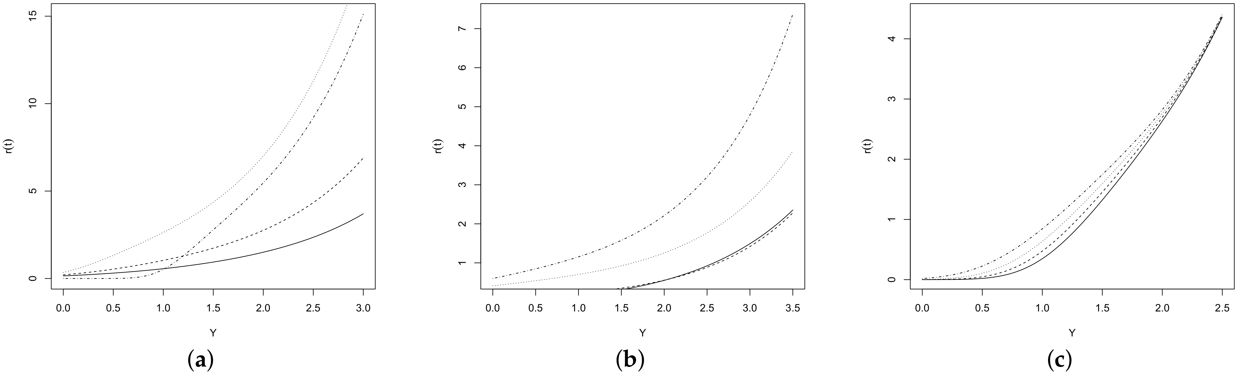
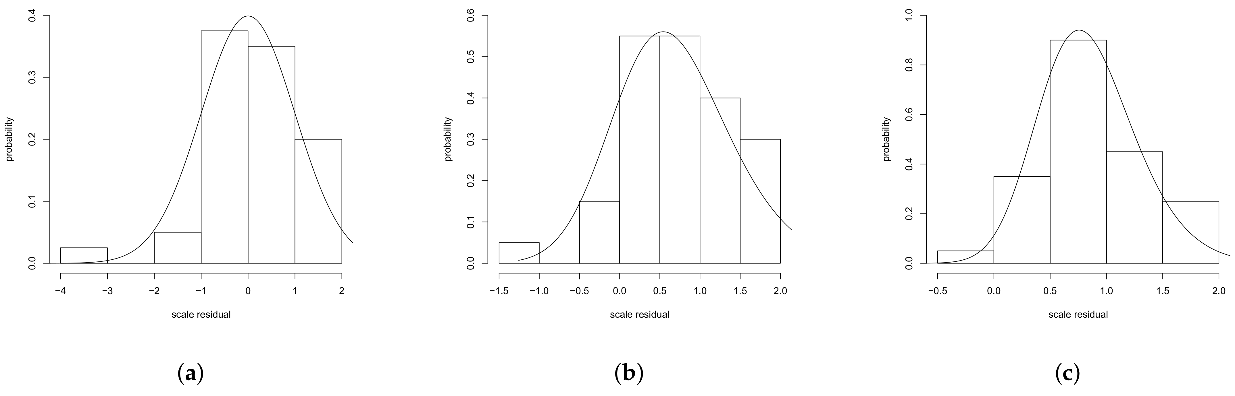
5.1. Application 1: Times to Failure

The data sets are of times to failure (T) in rolling contact fatigue of ten hardened steel specimens tested at each of four values of four contact stress points (x). The data were obtained using a four-ball rolling contact test rig at the Princeton Laboratories of Mobil Research and Development Co. The data set was given initially in McCool [30] and reported in Chan et al. [31]. These data sets were also analyzed in Lemonte [25], who, like Chan et al. [31], considered the regression model

$$Y_i={\beta }_0+{\beta }_{1}log\left(X_i\right)+{ϵ}_i,i=1,\dots ,40.$$

For the regression model described above, we propose using the sinh-normal (SHN) distribution, skewed sinh-normal (SESN), and skewed sinh power-normal (SPESN) distributions for ${ϵ}_i$, $i=1,2,\dots ,n$. To compare the fitness of these models, we use the Akaike [32] criterion, namely

$$AIC=-2\widehat{\ell }(·)+2k,$$

where k is the number of parameters in the model. According to this criterion, the model that best fits the data is the one with the lowest AIC. The SESN model can be obtained as a special case of the SPESN model when $\alpha =1$. The estimates for the parameters of these models are presented in Table 2.

Table 2. MLE estimates for the SHN, SESN, and SPESN models.

Parameters	SHN	SESN	SPESN
$\gamma$	1.279 (0.143)	2.011 (0.313)	5.379 (0.189)
${\beta }_0$	0.097 (0.170)	−0.961 (0.166)	−2.620 (0.060)
${\beta }_0^{*}$		0.165	0.289
${\beta }_1$	−14.116 (1.571)	−13.870 (1.602)	−13.602 (1.579)
$\lambda$		1.642 (0.618)	−0.932 (0.174)
$\alpha$			13.889 (4.991)
AIC	129.235	125.360	122.917

According to the AIC criterion, the SPESN model presents the best fit to the data set. Making the correction in the intercept of the SPESN model, we find that ${\widehat{\beta }}_0^{*}=0.289$, so we estimate the vector ${\widehat{\theta }}^{*}={(0.289,-13.602)}^{\top }$. We can conclude that the regression model with SPESN error distribution provides a better fit than the regression model with SESN error distribution.

We consider now the problem of testing the null hypothesis of no difference between the SPESN model and the traditional SHN model, that is,

$$H_{01}:(\lambda ,\alpha )=(0,1)\mathrm{versus}{H}_{11}:(\lambda ,\alpha )\ne (0,1)$$

using the likelihood ratio statistics (models are nested)

$${\mathsf{\Lambda }}_1=\frac{L_{SHN}\left(\widehat{\mathbf{\theta }}\right)}{L_{SPESN}\left(\widehat{\mathbf{\theta }}\right)}.$$

Numerical evaluations indicate that

$$-2log\left({\mathsf{\Lambda }}_1\right)=-2(-59.951+56.458)=6.986,$$

which is greater than the 5% critical value 5.991. Therefore, the null hypothesis is rejected and we conclude that the SPESN model (which involves two extra parameters, making it more flexible in terms of asymmetry and kurtosis) fits the data better (in fact, much better) than the SHN model.

The SPESN model is also compared to the SESN model by testing the hypothesis

$$H_{02}:\alpha =1\mathrm{versus}{H}_{12}:\alpha \ne 1,$$

respectively, using the likelihood ratio statistics ${\mathsf{\Lambda }}_2=\frac{{\ell }_{SESN}\left(\widehat{\mathbf{\theta }}\right)}{{\ell }_{SPESN}\left(\widehat{\mathbf{\theta }}\right)}$ After numerical evaluations, we obtain $-2log\left({\mathsf{\Lambda }}_2\right)=4.886$, which is greater than critical value ${\chi }_{1,95\%}^2=3.841,$ so that $H_{02}$ is rejected at the 5% critical value.

Note that the skewed log-linear Birnbaum–Saunders alpha-power model provides better fit to the data set the corresponding ones for the remaining models.

To confirm the good fit of the distributions used for the error term, we plotted the transformed standardized residual scale $Z_i=(2/\gamma )sinh(Y_i-x^{\top }$ $\mathbf{\beta }$ $)/2$ for the distribution of the estimated errors. Under this scale, the distribution of Z is normal for the SHN model, while for the SESN model, Z is the ordinary SN distribution and for the SPESN model, Z is PESN distribution. Figure 5 depicts the distribution for the scaled residuals Z for the set of models with the corresponding theoretical distributions.

Figure 5. Histogram for the scaled residuals Z, from the fitted models. (a) SHN, (b) SESN and (c) SPESN.

Figure 6 shows the qq-plots for the scaled residuals Z for the set of models SSN and SESN with the indicated theoretical distributions. One can see the good fit of the model with errors SPESN. Thus, this model is presented as a viable alternative to study data when the distribution of the response variable is asymmetric.

Figure 6. Qq-plots for the scaled residuals Z, from the fitted models. (a) SESN and (b) SPESN.

5.2. Application 2: Patients with Advanced Lung Cancer Status

The second application reported is related to the censored data set presented in Kalbfleisch and Prentice [33]. The uncensored data set under study corresponds to 128 male patients with advanced lung cancer status. The study aims at explaining the survival time T (in days) using a regression model. The explanatory variables that we consider were the following: a randomized measure of patients condition (Karnofsky). The data set was also analyzed in Martínez-Flores et al. [19]. Consider the regression model

$$Y_i={\beta }_0+{\beta }_{1}log\left(x_1\right)+{\beta }_{4}log\left(x_4\right)+{ϵ}_i,i=1,\dots ,128.$$

where $\left(x_1\right)$ is 10–30 fully randomized, 40–60 partially, and 70–90 patient’s ability for selfcare and $x_4$ histologic tumor squamous type: dichotomized as 1 for “yes” and 0 for “no” The estimates for the parameters of these models are presented in Table 3.

Table 3. MLE estimates for the SHN, SESN, and SPESN models.

Parameters	SHN	SESN	SPESN
$\gamma$	2.412 (0.153)	6.963 ( 2.185)	43.489 (19.792)
${\beta }_0$	1.524 (0.837)	−1.356 ( 0.713)	−5.678 (0.954)
${\beta }_1$	0.041 ( 0.015)	0.034 (0.007)	0.033 (0.004)
${\beta }_2$	−0.129 ( 0.509)	0.488 ( 0.305)	0.5776 (0.194)
$\lambda$		8.505 (5.523)	9.793 (16.669)
$\alpha$			2.468 (0.306)
AIC	322.208	193.285	154.786

According to the AIC criterion, the SPESN model presents the best fit to the data set. We can conclude that the regression model with SPESN error distribution provides a better fit than the regression model with SESN error distribution.

We consider now the problem of testing the null hypothesis of no difference between the SPESN model and the traditional SHN model, using the likelihood ratio statistics (models are nested) ${\mathsf{\Lambda }}_1=\frac{L_{SHN}\left(\widehat{\mathbf{\theta }}\right)}{L_{SPESN}\left(\widehat{\mathbf{\theta }}\right)}$. After numerical evaluations, we obtain $-2log\left({\mathsf{\Lambda }}_1\right)=169.422$, which is greater than the 5% critical value 5.991. Therefore, the null hypothesis is rejected and we conclude that the SPESN model (which involves two extra parameters, making it more flexible in terms of asymmetry and kurtosis) fits the data better (in fact, much better) than the SHN model. The SPESN model is also compared to the SESN model by testing the hypothesis, using the likelihood ratio statistics ${\mathsf{\Lambda }}_2=\frac{{\ell }_{SESN}\left(\widehat{\mathbf{\theta }}\right)}{{\ell }_{SPESN}\left(\widehat{\mathbf{\theta }}\right)}$ After numerical evaluations, we obtain $-2log\left({\mathsf{\Lambda }}_2\right)=39.495$, which is greater than critical value ${\chi }_{1,95\%}^2=3.841,$ so that $H_{02}$ is rejected at the 5% critical value.

Note that skewed log-linear Birnbaum–Saunders alpha-power model provides better fit to the data set the corresponding ones for the remaining models.

To confirm the good fit of the distributions used for the error term, we plotted the transformed standardized residual scale $Z_i=(2/\gamma )sinh(Y_i-x^{\top }$ $\mathbf{\beta }$ $)/2$ for the distribution of the estimated errors. Under this scale, the distribution of Z is normal for the SHN model, while for the SESN model, Z is the ordinary SN distribution and for the SPESN model, Z is PESN distribution. Figure 7 depicts the distribution for the scaled residuals Z for the set of models with the corresponding theoretical distributions.

Figure 7. Histogram for the scaled residuals Z, from the fitted models. (a) SHN, (b) SESN and (c) SPESN.

Figure 8 shows the qq-plots for the scaled residuals Z for the set of models SSN and SESN with the indicated theoretical distributions. One can see the good fit of the model with errors SPESN. Thus, this model is presented as a viable alternative to study data when the distribution of the response variable is asymmetric.

Figure 8. Qq-plots for the scaled residuals Z, from the fitted models. (a) SESN and (b) SPESN.

6. Conclusions

This paper introduced an extension of the log-linear Birnbaum–Saunders model by replacing the sin-normal distribution for the error term by the skew-sinh-power-normal distribution. Some features of the new model are:

• The introduction of two extra shape parameters makes the error distribution more flexible, allowing it to incorporate additional kurtosis and asymmetry.
• Maximum likelihood properties of large samples such as consistency and asymptotic normality were established.
• A simulation study was performed to evaluate of the ML estimations. As expected, the bias and standard deviation of our estimation decrease as the sample size n increases.
• In the applications, AIC criteria statistics are used. These criteria indicate that the model that best fit the data is SPESN model.
• A Bayesian approach will be worked on in a future work.

References

- Fang, K.T.; Zhang, Y.T. Generalized Multivariate Analysis; Sciences Press: Beijing, China; Springer: Berlin, Germany, 1990. [Google Scholar]
- Fang, K.T.; Kotz, S.; Ng, K.W. Symmetric Multivariate and Related Distribution; Chapman and Hall: London, UK, 1990. [Google Scholar]
- Gupta, A.K.; Varga, T. Elliptically Contoured Models in Statistics; Kluwer Academic Publishers: Boston, MA, USA, 1993. [Google Scholar]
- Kelker, D. Distribution Theory of Spherical Distributions and a Location Scale Parameter Generalization. Sankhya Ser. A 1970, 32, 419–430. [Google Scholar]
- Cambanis, S.; Huang, S.; Simons, G. On the Theory of Elliptically Contoured Distributions. J. Multivar. Anal. 1981, 11, 365–385. [Google Scholar] [CrossRef] [Green Version]
- Arellano-Valle, R. Distribuções Elipticas: Propriedades, Inferencia e Aplicações a Modelos de Regressão. Ph.D. Thesis, São Paulo University, São Paulo, Brazil, 1994, unpublished (In Portuguese). [Google Scholar]
- Lange, K.; Little, R.; Taylor, J. Robust statistical modelling using the t distribution. J. Am. Stat. Assoc. 1989, 84, 881–896. [Google Scholar]
- Arellano-Valle, R.; Bolfarine, H. On some characterizations of the Studen-t distribution. Stat. Probab. Lett. 1995, 25, 79–85. [Google Scholar] [CrossRef]
- Azzalini, A. A class of distributions which includes the normal ones. Scand. J. Stat. 1985, 12, 171–178. [Google Scholar]
- Owen, D.B. Tables for computing bi-variate normal probabilities. Ann. Math. Stat. 1956, 27, 1075–1090. [Google Scholar] [CrossRef]
- Durrans, S.R. Distributions of fractional order statistics in hydrology. Water Resour. Res. 1992, 28, 1649–1655. [Google Scholar] [CrossRef]
- Birnbaum, Z.W.; Saunders, S.C. A New Family of Life Distributions. J. Appl. Probab. 1969, 6, 319–327. [Google Scholar] [CrossRef]
- Birnbaum, Z.W.; Saunders, S.C. Estimation for a family of life distributions with applications to fatigue. J. Appl. Probab. 1969, 6, 328–347. [Google Scholar] [CrossRef]
- Díaz-García, J.A.; Leiva-Sánchez, V. A new family of life distributions based on the elliptically contoured distributions. J. Stat. Plan. Inference 2005, 128, 445–457. [Google Scholar] [CrossRef]
- Vilca-Labra, F.; Leiva-Sanchez, V. A new fatigue life model based on the family of skew-elliptical distributions. Commun. Stat. Theory Methods 2006, 35, 229–244. [Google Scholar] [CrossRef]
- Lachos, V.H.; Bolfarine, H.; Arellano-Valle, R.B.; Montenegro, L.C. Likelihood-based inference for multivariate skew-normal regression models. Commun. Stat. Theory Methods 2007, 36, 1769–1786. [Google Scholar] [CrossRef]
- Castillo, N.; Gomez, H.W.; Bolfarine, H. Epsilon Birnbaum-Saunders distribution family: Properties and inference. Stat. Pap. 2011, 52, 871–883. [Google Scholar] [CrossRef]
- Gómez, H.W.; Olivares, J.; Bolfarine, H. An extension of the generalized Birnbaum-Saunders distribution. Stat. Probab. Lett. 2009, 79, 331–338. [Google Scholar] [CrossRef]
- Martínez-Flórez, G.; Bolfarine, H.; Gómez, H.W. The Log-Linear Birnbaum-Saunders Power Model. Methodol. Comput. Appl. Probab. 2017, 19, 913–933. [Google Scholar] [CrossRef]
- Moreno-Arenas, G.; Martínez-Flórez, G.; Barrera-Causil, C. Proportional hazard Birnbaum-Saunders distribution with application to the survival data analysis. Rev. Colomb. Estad. 2016, 39, 129–147. [Google Scholar] [CrossRef]
- Rieck, J.R.; Nedelman, J.R. A log-linear model for the Birnbaum-Saunders distribution. Technometrics 1991, 33, 51–60. [Google Scholar]
- Galea, M.; Leiva, V.; Paula, G. Influence diagnostics in log-Birnbaum-Saunders regression models. J. Appl. Stat. 2004, 31, 1049–1064. [Google Scholar] [CrossRef]
- Barros, M.; Paula, G.A.; Leiva, V. A new class of survival regression models with heavy-tailed errors: Robustness and diagnostics. Lifetime Data Anal. 2008, 14, 316–332. [Google Scholar] [CrossRef] [PubMed]
- Leiva, V.; Vilca, F.; Balakrishnan, N.; Sanhueza, A. A Skewed Sinh-Normal Distribution and Its Properties and Application to Air Pollution. Commun. Stat. Theory Methods 2010, 39, 426–443. [Google Scholar] [CrossRef]
- Lemonte, A.J. A log-Birnbaum-Saunders regression model with asymmetric errors. J. Stat. Comput. Simul. 2012, 82, 1775–1787. [Google Scholar] [CrossRef] [Green Version]
- Santana, L.; Vilca, F.; Leiva, V. Influence analysis in skew-Birnbaum-Saunders regression models and applications. J. Appl. Stat. 2011, 38, 1633–1649. [Google Scholar] [CrossRef]
- Martínez-Flórez, G.; Bolfarine, H.; Gómez, Y.M.; Gómez, H.W. A unification of families of Birnbaum-Saunders distributions with applications. REVSTAT Stat. J. 2020, 18, 637–660. [Google Scholar]
- Chaibub Neto, E.; Branco, M. Bayesian Reference Analysis for Binomial Calibration Problem; IME-USP: São Paulo, Brazil, 2003. [Google Scholar]
- Prudnikov, A.P.; Brychkov, Y.A.; Marichev, O.I. Integrals and Series; Gordon and Breach Science Publishers: Amsterdam, The Netherlands, 1990; Volume 1–3. [Google Scholar]
- McCool, J.I. Confidence limits for Weibull regression with censored data. IEEE Trans. Reliab. 1980, 29, 145–150. [Google Scholar] [CrossRef]
- Chan, P.S.; Ng, H.K.T.; Balakrishnan, N.; Zhou, Q. Point and interval estimation for extreme-value regression model under Type-II censoring. Comput. Stat. Data Anal. 2008, 52, 4040–4058. [Google Scholar] [CrossRef]
- Akaike, H. A new look at statistical model identification. IEEE Trans. Autom. Control 1974, AU-19, 716–722. [Google Scholar] [CrossRef]
- Kalbfleisch, J.D.; Prentice, R.L. The Statistical Analysis of Faiture Time Data; Wiley: New York, NY, USA, 2002. [Google Scholar]
Publisher’s Note: MDPI stays neutral with regard to jurisdictional claims in published maps and institutional affiliations. |
© 2021 by the authors. Licensee MDPI, Basel, Switzerland. This article is an open access article distributed under the terms and conditions of the Creative Commons Attribution (CC BY) license (https://creativecommons.org/licenses/by/4.0/).