Semiclassical Spectral Series Localized on a Curve for the Gross–Pitaevskii Equation with a Nonlocal Interaction

Abstract

We propose the approach to constructing semiclassical spectral series for the generalized multidimensional stationary Gross–Pitaevskii equation with a nonlocal interaction term. The eigenvalues and eigenfunctions semiclassically concentrated on a curve are obtained. The curve is described by the dynamic system of moments of solutions to the nonlocal Gross–Pitaevskii equation. We solve the eigenvalue problem for the nonlocal stationary Gross–Pitaevskii equation basing on the semiclassical asymptotics found for the Cauchy problem of the parametric family of linear equations associated with the time-dependent Gross–Pitaevskii equation in the space of extended dimension. The approach proposed uses symmetries of equations in the space of extended dimension.

1. Introduction

The collective modes of coherent quantum atom ensembles in the Bose–Einstein condensate (BEC) confined by a trap field in the mean-field approximation are described by the nonlinear Schrödinger equation, the Gross–Pitaevskii equation (GPE) (see, e.g., [1,2,3,4]):

$$\begin{array}{c}{\displaystyle \left\{-i\hslash {\partial }_t-\frac{{\hslash }^2}{2m}\Delta +V_{tr}\left(\overrightarrow{x}\right)+\varkappa \widehat{W}[\Psi ](\overrightarrow{x},t)\right\}\Psi (\overrightarrow{x},t)=0.}\hfill \end{array}$$

(1)

Here, ${\displaystyle {\partial }_t=\frac{\partial }{\partial t}}$, $\Delta$ is the Laplace operator, m is the particle mass, $\varkappa$ is the nonlinearity parameter, $V_{tr}\left(\overrightarrow{x}\right)$ is the external field (trap) potential, the function $\Psi (\overrightarrow{x},t)$ is the macroscopic wavefunction of the condensate (the order parameter) such that $|\Psi (\overrightarrow{x},t){|}^2$ is proportional to the BEC density and its phase gradient is proportional to the BEC velocity. For the sake of simplicity, we omit the argument ℏ of the function $\Psi (\overrightarrow{x},t,\hslash )$ in formulas where it does not cause the confusion.The nonlinear interaction operator $\widehat{W}[\Psi ](\overrightarrow{x},t)$ in (1) is usually chosen as

$$\begin{array}{c}\hfill \widehat{W}[\Psi ](\overrightarrow{x},t)={\widehat{W}}_{local}[\Psi ](\overrightarrow{x},t)=g{|\Psi (\overrightarrow{x},t)|}^2\end{array}$$

(2)

and it describes the local interaction with $g=4\pi {\hslash }^{2}a/m$ where a is the s-wave scattering length. However, to take into account long-range interaction, the nonlocal operators are considered here

$$\begin{array}{c}\hfill {\displaystyle \widehat{W}[\Psi ](\overrightarrow{x},t)={\widehat{W}}_{nonlocal}[\Psi ](\overrightarrow{x},t)=\underset{{\mathbb{R}}^n}{\int }W(\overrightarrow{x},\overrightarrow{y}){|\Psi (\overrightarrow{y},t)|}^{2}d\overrightarrow{y}.}\end{array}$$

(3)

The local operator ${\widehat{W}}_{local}$ of (2) can be treated as the limit of the nonlocal version (3) with a delta-like function $W(\overrightarrow{x},\overrightarrow{y})$ that corresponds to the short-range interaction. Some applications in physics, specifically the BEC with the dipolar-to-dipolar interaction [5,6,7,8], require accounting the long-range interaction when one can notrequiring accounting the long-range interaction do not allow one to get rid of nonlocality for the sake of simplicity. In these cases, the combination of the local and nonlocal terms is often used. We call Equation (1) with the term ${\widehat{W}}_{local}$ the local GPE, and with ${\widehat{W}}_{nonlocal}$ the nonlocal GPE.

Substitution of $\Psi (\overrightarrow{x},t)=exp\left[\frac{-i\mu t}{\hslash }\right]\psi \left(\overrightarrow{x}\right)$ into Equation (1) yields the time- independent GPE

$${\displaystyle \left\{-\frac{{\hslash }^2}{2m}\Delta +V_{tr}\left(\overrightarrow{x}\right)+\varkappa \widehat{W}\left[\psi \right]\left(\overrightarrow{x}\right)\right\}\psi \left(\overrightarrow{x}\right)=\mu \psi \left(\overrightarrow{x}\right),}$$

(4)

which describes the stationary states of the BEC. If solutions $\psi \left(\overrightarrow{x}\right)$ of (4) are restricted to the unit norm

$${\displaystyle \left|\right|\psi \left(\overrightarrow{x}\right){\left|\right|}^2=\underset{{\mathbb{R}}^n}{\int }{\left|\psi \left(\overrightarrow{x}\right)\right|}^{2}d\overrightarrow{x}=1,}$$

(5)

then eigenvalues $\mu$ of the nonlinear eigenvalue problem (4) and (5) correspond to the chemical potential and eigenfunctions $\psi \left(\overrightarrow{x}\right)$ minimize the energy functional

$${\displaystyle E\left[\psi \right]=\underset{{\mathbb{R}}^n}{\int }\left[\frac{{\hslash }^2}{2m}|\nabla \psi \left(\overrightarrow{x}\right){|}^2+V_{tr}\left(\overrightarrow{x}\right)|\psi \left(\overrightarrow{x}\right){|}^2+\frac{\varkappa }{2}\widehat{W}\left[\psi \right]\left(\overrightarrow{x}\right){\left|\psi \left(\overrightarrow{x}\right)\right|}^2\right]d\overrightarrow{x},}$$

(6)

where E is the energy per the BEC particle. The ground state solution corresponds to the global minimum of the functional (6) while the exited states meet the local minima [9,10].

For the weak interaction (a small parameter $\varkappa$), the stationary solutions can be found using the perturbation theory as a correction to solutions of the so-called associated linear Schödinger equation that inherits the GPE linear part and has not the interaction term, i.e., it is the Equation (4) with $\varkappa =0$. Solutions of the GPE obtained in this way are termed solutions with linear counterpart in [11]. The opposite limit of strong nonlinearity was also considered using the Thomas–Fermi approximation when the kinetic term can be ignored and the local GPE (4) takes the form of an algebraic equation. For the nonlocal case, the GPE (4) becomes an integral equation. Moreover, it was shown that there are stationary solutions of the local GPE that do not correspond to any eigenfunctions of the associated linear Schödinger equation for multiwell external potential in [12] (the GPE solutions without linear counterpart).

The minima of the functional (6) can be found numerically by iterative procedure (see, e.g., the review in [13] and references therein). The issue is that the iterative procedure needs a proper initial approximation for the respective stationary states (4). For the weak nonlinearity, the stationary states of the associated linear Schrödinger equation can be used as the initial data, and, for the strong nonlinearity, the initial data can be obtained from the Thomas–Fermi approximation [9,14,15]. Numerical methods are usually limited to calculating only the ground state [13] and do not allow one to construct spectral series in the general case.

The study of the GPE solutions with and without linear counterpart was continued in [16,17,18,19,20].

Note that the solutions with linear counterpart inherit the symmetries of the external field potential while these symmetries are broken for solutions without linear counterpart.

In order to avoid the limitations of the weak or strong nonlinearity, the semiclassical approximation can be used. For example, in [21], the semiclassical approximation was used to study the non-stationary local GPE with the special type of external field and different orders of the nonlinear term.

Here, we propose an approach to the spectral problem (4) that deals with the arbitrary strength of the nonlinearity and is applicable for a wide range of the external fields in n-dimensional nonlocal GPE. Moreover, we study the nonlocal GPE solutions localized on curves reflecting the BEC topological features. We apply the well-known WKB-Maslov theory of semiclassical approximation [22,23,24] to the problem under consideration. The approach to the eigenvalue problem (4) and (5) is based on [25], where the leading term of semiclassical asymptotics for the Cauchy problem has been constructed explicitly in a class of functions localized in a neighborhood of a curve in the phase space of a dynamic system of moments of the nonlocal GPE solution termed the Hamilton–Ehrenfest system. The last one for the n-dimensional manifolds in the phase space was studied in [26,27,28]. As opposed to the linear case ($\varkappa =0$ in (4)), the variance matrix of the solutions constructed in [25] may be bounded due to the nonlinearity. Such solutions of the Cauchy problems are termed the semiclassical soliton-type solutions [29], and we use exactly such particular solutions for the construction of the spectral series of the nonlocal GPE.

Differ toDiffering from the associated linear Schödinger equation in the sense of [11], our method uses a parametric family of the associated linear Gross–Pitaevskii equations that include terms corresponding to both the external field and the interaction. Among the solutions of these equations, the solution of the initial nonlinear GPE (4) can be found.

Our consideration is not limited to the convolution nonlinearity with the kernel $W(\overrightarrow{x},\overrightarrow{y})=W(\overrightarrow{x}-\overrightarrow{y})$, which naturally arise in the BEC application. Although the convolution nonlinearity is usually simpler for calculations, it is unsubstantial for our approach. Moreover, the consideration of the wider class of kernels $W(\overrightarrow{x},\overrightarrow{y})$ allows one to apply this approach to the GPE with the modulated nonlinearity that was studied in [18,19].

The WKB-Maslov method sometimes leads to quite complex classical equations (the Hamilton–Ehrenfest system) that need semi-analytical considerations. However, the development of numerical-analytical math packages, such as Wolfram Mathematica, breathed new life into the semiclassical method [30]. In [31], it was applied to the nonlocal generalization of the Fokker–Plank equation with solutions localized on a zero-dimensional manifold (a point). In [32,33], the WKB-Maslov method allowed to construct asymptotic solutions concentrated on curves for the nonlocal Fisher–Kolmogorov–Petrovskii–Piskunov equation. Semiclassical spectral series were constructed in [34,35] for the Hartree type equation with the special type of the external potential $V_{tr}$.

Our method focuses on formal mathematical structures, so it is applicable for constructing solutions of a wider class of equations. In particular, the approach can be generalized for nonlinear Schrödinger-like equations such as Lugiato–Lefever equation, which is an amplitude equation for an optical pulse in the pumped ring resonator [36]. The interest in this equation was encouraged by discovery of the frequency comb associated with the Kerr temporal solitons [37,38,39]. The results of our paper may be of value for the theoretical study of the Bose–Einstein condensation phenomena that occurs in a gas of atoms and of various quasiparticles [3,40,41,42,43,44]. Note that the conception of condensation is even involved in the study of dark matter [45,46].

The paper is structured as follows. In Section 2, we describe the asymptotic particular solutions of the non-stationary nonlocal GPE concentrated on curves. In Section 3, we construct the asymptotic solutions of the stationary nonlocal GPE based on the Section 2. In Section 3, the semiclassical spectral series are obtained. In Section 4, our formalism is illustrated by an example for the specific 2D stationary nonlocal GPE. The semiclassical solutions of the spectral problem for this equation are obtained in the analytical form. In Section 5, the concluding remarks are given. In Appendix, the auxiliary equations involved are given.

2. Nonlocal Gross–Pitaevskii Equation

The semiclassical approach to the spectral problem (4) can be developed for the nonlocal stationary GPE of a more general form

$$\begin{array}{c}\left\{H\left(\widehat{z}\right)\left[\psi \right]-\mu (\hslash )\right\}\psi \left(\overrightarrow{x}\right)=0,\\ {\displaystyle H\left(\widehat{z}\right)\left[\psi \right]=V\left(\widehat{z}\right)+\varkappa \underset{{\mathbb{R}}^n}{\int }W(\overrightarrow{x},\overrightarrow{y}){\left|\psi \left(\overrightarrow{y}\right)\right|}^{2}d\overrightarrow{y}.}\end{array}$$

(7)

Here, $\widehat{z}=(\widehat{\overrightarrow{p}},\overrightarrow{x})$, $\overrightarrow{x}\in {\mathbb{R}}^n$, $\widehat{\overrightarrow{p}}=-i\hslash {\partial }_{\overrightarrow{x}}$, and $V\left(\widehat{z}\right)$ is a linear partial differential operator depending on $\widehat{z}$ with a symbol $V\left(z\right)=V(\overrightarrow{p},\overrightarrow{x})$ smoothly depending on $\overrightarrow{p}$ and $\overrightarrow{x}$ ($\overrightarrow{p}\in {\mathbb{R}}^n$). Our approach to the problem (7) relies on the method proposed in [25] for solution of the Cauchy problem in the semiclassical approximation for the non-stationary nonlocal GPE:

$$\begin{array}{c}\left\{-i\hslash {\partial }_t+H\left(\widehat{z}\right)[\Psi ]\right\}\Psi (\overrightarrow{x},t)=0,\\ \Psi (\overrightarrow{x},t){|}_{t=0}=\psi \left(\overrightarrow{x}\right).\end{array}$$

(8)

This method allows one to construct the asymptotical solutions to the problem (8) in the class of functions semiclassically concentrated on curves of the phase space of the dynamical system of moments of the desired solution.

The core idea of the approach proposed is as follows. The method of [25] provides a practical possibility to select from the set of asymptotical solutions $\Psi (\overrightarrow{x},t)$ to the Cauchy problem (8), found for various initial functions $\psi \left(\overrightarrow{x}\right)$, those $\Psi (\overrightarrow{x},t)$ that have the form

$${\displaystyle \Psi (\overrightarrow{x},t)=exp\left[-\frac{i}{\hslash }\mu t\right]·\psi \left(\overrightarrow{x}\right).}$$

(9)

In the process of finding the functions (9), we come to $\psi \left(\overrightarrow{x}\right)$ and $\mu$ which are the eigenfunctions and eigenvalues of the problem (7).

Consider solutions of (8) concentrated in a vicinity of the one-dimensional manifold ${\Lambda }_t^1$ (the curve) in the $2n$-dimensional phase space ${\mathbb{M}}^{2n}={\mathbb{R}}^n\times {\mathbb{R}}^n$, $\overrightarrow{p}\in {\mathbb{R}}^n$, $\overrightarrow{x}\in {\mathbb{R}}^n$:

$$\begin{array}{c}{\Lambda }_t^1=\{z=(\overrightarrow{p},\overrightarrow{x})=Z(t,s,\hslash )=\left(\overrightarrow{P}(t,s,\hslash ),\overrightarrow{X}(t,s,\hslash )\right)|\\ s\in [0,\omega T],t\in [0,T]\},T,\omega >0.\end{array}$$

(10)

Here, s is the curve ${\Lambda }_t^1$ parameter and:

$$Z(t,s,\hslash )=Z(t,s)+\hslash Z^{\left(1\right)}(t,s)+\mathrm{O}\left({\hslash }^{3/2}\right).$$

(11)

For the functions $\Psi$ semiclassically concentrated on the curve ${\Lambda }_t^1$, the dynamics of the curve in the limits $\hslash \to 0$ is determined by the $(1,1)$-type Hamilton–Ehrenfest system (the term $(1,1)$ implies that the parameter s is a one-dimensional variable and the vector $Z(s,t)$ corresponds to the first order moments of the function $\Psi (\overrightarrow{x},t)$, see [25] for details):

$$\left\{\begin{array}{c}\dot{\overrightarrow{X}}(t,s)=V_{\overrightarrow{p}}\left(Z(t,s)\right),\hfill \\ {\displaystyle \dot{\overrightarrow{P}}(t,s)=-V_{\overrightarrow{x}}\left(Z(t,s)\right)-\frac{{\varkappa \left|\right|\Psi \left|\right|}^2}{\omega T}\underset{0}{\overset{\omega T}{\int }}{W}_{\overrightarrow{x}}\left(\overrightarrow{X}(t,s),\overrightarrow{X}(t,r)\right)dr.}\hfill \end{array}\right.$$

(12)

Here, $\left|\right|\Psi \left|\right|$ is the $L_2$-norm, which is conserved for exact solutions of the non-stationary nonlocal GPE (8). Hereinafter, for the sake of simplicity, we will use the unit normalization $\left|\right|\Psi \left|\right|=1$.

The class ${\mathcal{J}}_{\hslash }^{\tau }$ of functions semiclassically concentrated on curves ${\Lambda }^1$ is given by

$$\begin{array}{cc}& {\mathcal{J}}_{\hslash }^{\tau }=\left\{\Phi :\Phi (\overrightarrow{x},t,\hslash )=\chi (\overrightarrow{x},t,s,\hslash ){|}_{s=\omega \tau (\overrightarrow{x},t)},\chi (\overrightarrow{x},t,s,\hslash )\in {\mathcal{P}}_{\hslash }^t\left(s\right)\right\},\end{array}$$

(13)

where ${\mathcal{P}}_{\hslash }^t$ is a class of trajectory-concentrated functions [47]:

$$\begin{array}{c}\hfill {\displaystyle {\mathcal{P}}_{\hslash }^t\left(s\right)=\left\{\chi :\chi (\overrightarrow{x},t,s,\hslash )=\phi \left(\frac{\Delta \overrightarrow{x}}{\sqrt{\hslash }},t,s,\hslash \right)exp\left[\frac{i}{\hslash }\left(S(t,s,\hslash )+\langle \overrightarrow{P}(t,s),\Delta \overrightarrow{x}\rangle \right)\right]\right\}.}\end{array}$$

(14)

In this definition, the function $\phi (\overrightarrow{\xi },t,s,\hslash )$ belongs to a Schwarz space $\mathbb{S}$ in the variable $\overrightarrow{\xi }\in {\mathbb{R}}^n$, smoothly depends on t and s, and regularly depends on $\sqrt{\hslash }$ as $\hslash \to 0$; the function $S(t,s,\hslash )$ together with functions $Z(t,s)=(\overrightarrow{P}(t,s),\overrightarrow{X}(t,s))$ define the class and are to be determined; the family of hypersurfaces $s=\omega \tau (\overrightarrow{x},t)$ are given by relation [23,24]

$$〈{\overrightarrow{X}}_s(t,s),\Delta \overrightarrow{x}〉=0,\Delta \overrightarrow{x}=\overrightarrow{x}-\overrightarrow{X}\left(t,s\right).$$

(15)

Hereinafter, we assume that

$$\mathrm{rank}{\overrightarrow{X}}_s(t,s)=1.$$

(16)

This condition ensures the nondegeneracy of the localization curve (10) and the nonsingularity of the BEC density on the curve.

The construction of solutions of the form

$$\Psi (\overrightarrow{x},t)=\chi (\overrightarrow{x},t,s){|}_{s=\omega \tau (\overrightarrow{x},t)}$$

(17)

to the non-stationary GPE (8) in the class of functions ${\mathcal{J}}_{\hslash }^{\tau }$ in the semiclassical approximation with the accuracy of $\mathrm{O}\left({\hslash }^{3/2}\right)$ can be reduced to the solution of the associated linear GPE:

$$\begin{array}{cc}& {\displaystyle \left[-i\hslash {\partial }_t+H(t,s,\hslash )\left[g(t,s)\right]+\langle H_z(t,s),\Delta \widehat{z}\rangle +\frac{1}{2}\langle \Delta \widehat{z},H_{zz}(t,s)\Delta \widehat{z}\rangle \right]\chi (\overrightarrow{x},t,s)=0,}\end{array}$$

(18)

with the additional algebraic constraint

$$\begin{array}{c}\hfill {\widehat{a}}_0(t,s)\chi (\overrightarrow{x},t,s)=0.\end{array}$$

(19)

Here, we denoted

$$\begin{array}{cc}\hfill & {\displaystyle H\left(t,s,\hslash \right)\left[g(t,s)\right]=V\left(Z(t,s)\right)+\frac{\varkappa }{\omega T}\underset{0}{\overset{\omega T}{\int }}dr\{W\left(\overrightarrow{X}(t,s),\overrightarrow{X}(t,r)\right)+}\hfill \\ \hfill & {\displaystyle +\hslash 〈W_{\overrightarrow{y}}\left(\overrightarrow{X}(t,s),\overrightarrow{X}(t,r)\right),{\overrightarrow{X}}^{\left(1\right)}(t,r)〉+\frac{1}{2}\mathrm{Sp}\left[W_{yy}\left(\overrightarrow{X}(t,s),\overrightarrow{X}(t,r)\right)·{\sigma }_{xx}(t,r)\right]\},}\hfill \\ \hfill \\ \hfill & {\displaystyle H_z(t,s)=V_z\left(Z(t,s)\right)+\frac{\varkappa }{\omega T}\underset{0}{\overset{\omega T}{\int }}dr{W}_z\left(\overrightarrow{X}(t,s),\overrightarrow{X}(t,r)\right),W_z={\left(\overrightarrow{0},W_{\overrightarrow{x}}\right)}^{\top },}\hfill \\ \hfill & {\displaystyle H_{zz}(t,s)=V_{zz}\left(Z(t,s)\right)+\frac{\varkappa }{\omega T}\underset{0}{\overset{\omega T}{\int }}dr{W}_{zz}\left(\overrightarrow{X}(t,s),\overrightarrow{X}(t,r)\right),W_{zz}=\left(\begin{array}{cc}0& 0\\ 0& W_{xx}\end{array}\right),}\hfill \\ \hfill & {\widehat{a}}_0(t,s)=\langle {\overrightarrow{P}}_s(t,s),\Delta \overrightarrow{x}\rangle -\langle {\overrightarrow{X}}_s(t,s),\Delta \widehat{\overrightarrow{p}}\rangle ,\hfill \\ \hfill & \Delta \widehat{z}=(\Delta \widehat{\overrightarrow{p}},\Delta \overrightarrow{x})=\widehat{z}-Z(t,s),\hfill \end{array}$$

(20)

and functions $g(t,s)=(Z^{\left(1\right)}(t,s,\hslash )$, ${\Delta }_2(t,s))$, where ${\Delta }_2=\left(\begin{array}{cc}{\sigma }_{pp}& {\sigma }_{px}\\ {\sigma }_{xp}& {\sigma }_{xx}\end{array}\right)$, are the solutions of the second order Hamilton–Ehrenfest system with integration constants determined from the initial condition for the function $\chi (\overrightarrow{x},t,s)$. In general case, these functions are given by:

$$\begin{array}{c}{\displaystyle Z^{\left(1\right)}(t,s)=\frac{1}{\hslash }\langle \langle \Delta \widehat{z}\rangle \rangle ,{\Delta }_{2km}(t,\hslash )=〈〈\frac{1}{2}\left(\Delta {\widehat{z}}_k\Delta {\widehat{z}}_m+\Delta {\widehat{z}}_m\Delta {\widehat{z}}_k\right)〉〉,k,m=\overline{1,2n}.}\hfill \end{array}$$

(21)

Here, $\langle \langle \widehat{A}\rangle \rangle$ is the mean value of the operator with a Weyl symbol $A(z,t)$ in the class ${\mathcal{J}}_{\hslash }^{\tau }$:

$$\begin{array}{c}{\displaystyle \langle \langle \widehat{A}\rangle \rangle (t,s)=\frac{1}{\omega T}\underset{\mathbb{D}}{\int }{\chi }^{*}(\overrightarrow{x},t,s)A(\widehat{z},t)\chi (\overrightarrow{x},t,s)d\xi ,}\end{array}$$

(22)

where $\xi$ is $(n-1)$-dimensional vector of variables that complement the variable $s=\omega \tau (\overrightarrow{x},t)$ to form the coordinate system in ${\mathbb{R}}^n$, $\mathbb{D}$ is the domain of the variables $\xi$, and the operator $\widehat{z}$ acts subject to the condition $s=\mathrm{const}$.

The particular solution of (18) with auxiliary algebraic constraint (19) can be written in terms of solutions of the variational system, which is the linear Hamiltonian system:

$$\dot{a}(t,s)=J{H}_{zz}(t,s)a(t,s),$$

(23)

where $a(t,s)\in {\mathbb{C}}^{2n}$, $J=\left(\begin{array}{cc}0& -{\mathbb{I}}_{n\times n}\\ {\mathbb{I}}_{n\times n}& 0\end{array}\right)$ is unit symplectic matrix, (${\mathbb{I}}_{n\times n}$ is the unit $n\times n$-matrix). The function $a_0(t,s)=\dot{Z}(t,s)$ is the particular solutions of (23). Let $(n-1)$ linear independent solutions of (23) be known and satisfy the conditions

$$\begin{array}{c}\{a_0,a_k\}=0,\{a_0,a_k^{*}\}=0,\\ \{a_l,a_k\}=0,\{a_l^{*},a_k\}=2i{\delta }_{lk},l,k=\overline{1,(n-1)}.\end{array}$$

(24)

Here, ${\delta }_{lk}$ is the Kronecker symbol, $\{·,·\}$ is the skew-orthogonal product.

Denote $a_k(t,s)=\left({\overrightarrow{W}}_k(t,s),{\overrightarrow{Z}}_k(t,s)\right)$. Then, the particular solutions of (18) reads [47]

$$\begin{array}{c}{\displaystyle {\chi }_0(\overrightarrow{x},t,s)\left[g(t,s)\right]=\frac{N}{\sqrt{detC(t,s)}}exp\left\{\frac{i}{\hslash }\right[\underset{0}{\overset{t}{\int }}(\langle \overrightarrow{P}(\tau ,s),\dot{\overrightarrow{X}}(\tau ,s)\rangle -}\hfill \\ {\displaystyle -H(\tau ,s,\hslash )\left[g(t,s)\right])d\tau +\langle \overrightarrow{P}(t,s),\Delta \overrightarrow{x}\rangle +\frac{1}{2}\langle \Delta \overrightarrow{x},Q(t,s)\Delta \overrightarrow{x}\rangle ]\},}\hfill \end{array}$$

(25)

where N is the normalization coefficient, and

$$\begin{array}{c}Q(t,s)=B(t,s)C^{-1}(t,s),\hfill \\ B(t,s)=\left({\overrightarrow{P}}_s(t,s),{\overrightarrow{W}}_1(t,s),...,{\overrightarrow{W}}_{n-1}(t,s)\right)\in {\mathbb{C}}^{n\times n},\hfill \\ C(t,s)=\left({\overrightarrow{X}}_s(t,s),{\overrightarrow{Z}}_1(t,s),...,{\overrightarrow{Z}}_{n-1}(t,s)\right)\in {\mathbb{C}}^{n\times n}.\hfill \end{array}$$

(26)

The conditions (16) and (24) ensures the non-degeneracy of matrix $C(t,s)$. In order to make sure that function (40) satisfies the auxiliary constraint (19) it is enough to check the validity of the identity

$${\overrightarrow{P}}_s(t,s)-Q(t,s){\overrightarrow{X}}_s(t,s)={\overrightarrow{P}}_s(t,s)-B(t,s)C^{-1}(t,s){\overrightarrow{X}}_s(t,s)=0,$$

(27)

which results from the property

$$C^{-1}(t,s){\overrightarrow{X}}_s(t,s)={(1,0,...,0)}^{\top },$$

(28)

following from the definition of the matrix $C(t,s)$.

Let us introduce first order operators of the form

$$\begin{array}{c}{\displaystyle {\widehat{a}}_k(t,s)=\frac{1}{\sqrt{2\hslash }}\langle a_k(t,s),J^{\top }\Delta \widehat{z}\rangle ,}\hfill \\ {\displaystyle {\widehat{a}}_k^{+}(t,s)=\frac{1}{\sqrt{2\hslash }}\langle a_k^{*}(t,s),J^{\top }\Delta \widehat{z}\rangle ,k=\overline{1,n-1}.}\hfill \end{array}$$

(29)

Due to (24), the following commutation relations hold:

$$\begin{array}{c}[{\widehat{a}}_0,{\widehat{a}}_k]=[{\widehat{a}}_0,{\widehat{a}}_k^{+}]=[{\widehat{a}}_k,{\widehat{a}}_m]=[{\widehat{a}}_k^{+},{\widehat{a}}_m^{+}]=0,\\ {\widehat{a}}_k,{\widehat{a}}_m^{+}]={\delta }_{km},k,m=\overline{1,n-1}.\end{array}$$

(30)

These operators are the symmetry operators of (18) that preserve the property (19) of the solutions. Thus, the operators ${\widehat{a}}_k^{+}$, $k=\overline{1,n-1}$ are creation operators of (18), and the operators ${\widehat{a}}_k$, $k=\overline{0,n-1}$ are annihilation operators. The function $|0,t\rangle$ (40) is the “vacuum” solution. Let us construct the “occupation number representation” for (18) by determination of the following countable set of solutions:

$${\displaystyle {\chi }_{\nu }(\overrightarrow{x},t,s)=\prod _{k=1}^{n-1}\frac{1}{\sqrt{{\nu }_k!}}{\left({\widehat{a}}_k^{+}(t,s)\right)}^{{\nu }_k}{\chi }_0(\overrightarrow{x},t,s).}$$

(31)

Here, $\nu \in {\mathbb{Z}}_{+}^n$ is a $(n-1)$-dimensional multiindex, $\nu =({\nu }_1,{\nu }_2,...,{\nu }_{n-1})$, ${\nu }_k=\overline{0,\infty }$, $k=\overline{1,n-1}$:

$$\nu !=\prod _{k=1}^{n-1}{\nu }_k!,\overrightarrow{a}{}^{\nu }=\prod _{k=1}^{n-1}{a}_k^{{\nu }_k}.$$

(32)

In the next Section, we will construct stationary solutions of the GPE based on the solutions (31) and (25).

3. Stationary Solutions of the GPE

In order to obtain solutions that do not depend on time, we construct time-invariant curves. Let us consider curves determined by the following form of functions $Z(t,s)$:

$$\begin{array}{c}Z(t,s)=Z(t+s/\omega ),\hfill \\ Z(t+T)=Z\left(t\right),\hfill \end{array}$$

(33)

Here, a parameter $\omega$ is the ratio between the periods by s and by t. The curve ${\Lambda }_t^1$ determined by such the functions is mapped into itself with change of t, i.e., ${\Lambda }_t^1={\Lambda }^1$ does not depend on t. By the change of variables $(t+s/\omega )\to t$ and $(t+r/\omega )\to r$, the system (12) can be written in the following form:

$$\left\{\begin{array}{c}\dot{\overrightarrow{X}}\left(t\right)=V_{\overrightarrow{p}}\left(Z\left(t\right)\right),\hfill \\ {\displaystyle \dot{\overrightarrow{P}}\left(t\right)=-V_{\overrightarrow{x}}\left(Z\left(t\right)\right)-\frac{\varkappa }{T}\underset{0}{\overset{T}{\int }}{W}_{\overrightarrow{x}}\left(\overrightarrow{X}\left(t\right),\overrightarrow{X}\left(r\right)\right)dr.}\hfill \end{array}\right.$$

(34)

In this case, the equation of hypersurfaces $s=\omega \tau (\overrightarrow{x},t)$ has the form $s=\omega \tau \left(\overrightarrow{x}\right)+t$ or

$$t+s/\omega =\tau \left(\overrightarrow{x}\right).$$

(35)

Let the solutions of the second order Hamilton–Ehrenfest satisfy the relations $g(t,s)=g(t+s/\omega )$, $g(t+T)=g\left(t\right)$, i.e.

$$\begin{array}{c}{Z}^{\left(1\right)}(t,s)=({\overrightarrow{P}}^{\left(1\right)}(t,s),{\overrightarrow{X}}^{\left(1\right)}(t,s))=Z^{\left(1\right)}(t+s/\omega ),Z^{\left(1\right)}(t+T)=Z^{\left(1\right)}\left(t\right),\hfill \\ {\Delta }_2(t,s)={\Delta }_2(t+s/\omega ),{\Delta }_2(t+T)={\Delta }_2\left(t\right).\hfill \end{array}$$

(36)

The second order Hamilton–Ehrenfest system and the way of obtaining the functions satisfying the relations (36) are considered in the Appendix A.

For the solutions of the $(1,1)$-type Hamilton–Ehrenfest system satisfying (33), the variational system (23) reads

$$\dot{a}\left(t\right)=J{H}_{zz}\left(t\right)a\left(t\right),$$

(37)

where we put

$$a(t,s)=a(t+s/\omega ),$$

(38)

and made the change of the variable $(t+s/\omega )\to t$. Since $H_{zz}\left(t\right)$ is the periodic function, we can pose the Floquet problem for the variational system (37). We know at least one solution of the Floquet problem for (37), namely $a_0\left(t\right)=\dot{Z}\left(t\right)$ (the T-periodic solution). Let there be $(n-1)$ more linear independent solutions of the Floquet problem for (37) that satisfy the following Floquet conditions:

$$a_k(t+T)=exp\left[i{\Omega }_{k}T\right]a_k\left(t\right),\mathrm{Im}{\Omega }_k=0,k=\overline{1,(n-1)}$$

(39)

and the skew-orthogonality condition (24). Since only linearly stable ${\Lambda }^1$ are of interest for us, we consider the solutions of (37) with the real Floquet exponent ${\Omega }_k$.

If conditions (33), (36) and (38) are met, the particular solutions (25), (31) of (18) read ${\displaystyle {\chi }_{\nu }(\overrightarrow{x},t,s)\left[g_{\nu }(t+s/\omega )\right]=exp\left[-\frac{i}{\hslash }{\mu }_{\nu }t\right]{\chi }_{\nu }(\overrightarrow{x},t+s/\omega ,{\mu }_{\nu })\left[g_{\nu }(t+s/\omega )\right]}$, where

$$\begin{array}{c}{\displaystyle {\chi }_0(\overrightarrow{x},t,{\mu }_0)\left[g_0\left(t\right)\right]=\frac{N}{\sqrt{detC\left(t\right)}}exp\left\{\frac{i}{\hslash }\right[\underset{0}{\overset{t}{\int }}(\langle \overrightarrow{P}\left(r\right),\dot{\overrightarrow{X}}\left(r\right)\rangle -}\\ {\displaystyle -H(r,\hslash )\left[g_0\left(t\right)\right]+{\mu }_0(\hslash ))dr+\langle \overrightarrow{P}\left(t\right),\Delta \overrightarrow{x}\rangle +\frac{1}{2}\langle \Delta \overrightarrow{x},Q\left(t\right)\Delta \overrightarrow{x}\rangle ]\},}\end{array}$$

(40)

$$\begin{array}{c}{\displaystyle {\chi }_{\nu }(\overrightarrow{x},t,{\mu }_{\nu })\left[g_{\nu }\left(t\right)\right]=\prod _{k=1}^{n-1}\frac{1}{\sqrt{{\nu }_k!}}{\left({\widehat{a}}_k^{+}\left(t\right)\right)}^{{\nu }_k}{\chi }_0(\overrightarrow{x},t,{\mu }_{\nu })\left[g_{\nu }\left(t\right)\right].}\end{array}$$

(41)

Then, considering (9) and (35), the relation (17) is as follows:

$${\psi }_{\nu }\left(\overrightarrow{x}\right)={\chi }_{\nu }(\overrightarrow{x},t,{\mu }_{\nu })\left[g_{\nu }\left(t\right)\right]{|}_{t=\tau \left(\overrightarrow{x}\right)}.$$

(42)

The transition (42) from the extended $(n+1)$-dimensional space to the n-dimensional configuration space can give the multi-valued function $\psi \left(\overrightarrow{x}\right)$. However, the function $\psi \left(\overrightarrow{x}\right)$ is the single-valued one if the following periodicity condition holds:

$${\chi }_{\nu }(\overrightarrow{x},t+T,{\mu }_{\nu })\left[g_{\nu }\left(t\right)\right]={\chi }_{\nu }(\overrightarrow{x},t,{\mu }_{\nu })\left[g_{\nu }\left(t\right)\right].$$

(43)

In the next Section, we will study what constraints are caused by this condition.

4. Semiclassical Spectral Series

In view of the theorems given in Appendix B and relation (39), the condition (43) for solutions (40) and (41)The misprint in this reference was corrected reads [24]

$$\begin{array}{c}{\displaystyle \underset{0}{\overset{T}{\int }}\left[\langle \overrightarrow{P}\left(t\right),\dot{\overrightarrow{X}}\left(t\right)\rangle -H(t,\hslash )\left[g_{\nu }\left(t\right)\right]+{\mu }_{\nu }(\hslash )\right]dt=2\pi \hslash l+\hslash T\sum _{k=0}^{n-1}{\Omega }_k\left({\nu }_k+\frac{1}{2}\right),l\in \mathbb{Z}.}\hfill \end{array}$$

(44)

Let us denote $H(t,\hslash )\left[g\left(t\right)\right]=H^{\left(0\right)}\left(Z\left(t\right)\right)+\hslash H^{\left(1\right)}\left(t\right)\left[g\left(t\right)\right]$, where

$$\begin{array}{c}{\displaystyle H^{\left(0\right)}\left(Z\left(t\right)\right)=V\left(Z\left(t\right)\right)+\frac{\varkappa }{T}\underset{0}{\overset{T}{\int }}W\left(\overrightarrow{X}\left(t\right),\overrightarrow{X}\left(r\right)\right)dr,}\hfill \\ {\displaystyle H^{\left(1\right)}\left(t\right)\left[g\left(t\right)\right]=\frac{\varkappa }{T}\underset{0}{\overset{T}{\int }}dr(〈W_{\overrightarrow{y}}\left(\overrightarrow{X}\left(t\right),\overrightarrow{X}\left(r\right)\right),{\overrightarrow{X}}^{\left(1\right)}\left(r\right)〉+}\hfill \\ {\displaystyle +\frac{1}{2\hslash }\mathrm{Sp}\left[W_{yy}\left(\overrightarrow{X}\left(t\right),\overrightarrow{X}\left(r\right)\right)·{\sigma }_{xx}\left(r\right)\right]),}\hfill \end{array}$$

(45)

and assume

$$\mu (\hslash )={\mu }^{\left(0\right)}+\hslash {\mu }^{\left(1\right)}(\hslash ),$$

(46)

where ${\mu }^{\left(1\right)}(\hslash )$ regularly depends on ℏ.

We consider the periodic trajectories of the $(1,1)$-type Hamilton–Ehrenfest system with the period $T=T\left({\mu }^{\left(0\right)}\right)$ determined by the following integral of motion of (34):

$$\begin{array}{c}{H}^{\left(0\right)}\left(Z\left(t,T\left({\mu }^{\left(0\right)}\right)\right)\right)={\mu }^{\left(0\right)}.\hfill \end{array}$$

(47)

Then, the quantization condition (44) is satisfied if

$$\begin{array}{c}{\displaystyle \underset{0}{\overset{T\left({\mu }^{\left(0\right)}\right)}{\int }}\langle \overrightarrow{P}\left(t,T\left({\mu }^{\left(0\right)}\right)\right),\dot{\overrightarrow{X}}\left(t,T\left({\mu }^{\left(0\right)}\right)\right)\rangle dt=2\pi \hslash l,}\hfill \\ {\displaystyle {\mu }_{\nu }^{\left(1\right)}=\frac{1}{T}\underset{0}{\overset{T}{\int }}{H}^{\left(1\right)}\left(t\right)\left[g_{\nu }\left(t\right)\right]dt+\sum _{k=0}^{n-1}{\Omega }_k\left({\nu }_k+\frac{1}{2}\right).}\hfill \end{array}$$

(48)

The first equation in (48) implicitly determines ${\mu }^{\left(0\right)}$. The energy per particle for constructed semiclassical spectral series is given by

$$\begin{array}{c}{E}_{\nu }=E^{\left(0\right)}+\hslash E_{\nu }^{\left(1\right)}+\mathrm{O}\left({\hslash }^{3/2}\right),\hfill \\ {\displaystyle E^{\left(0\right)}=\frac{1}{T}\underset{0}{\overset{T}{\int }}dt\left[V\left(Z\left(t\right)\right)+\frac{1}{2}\frac{\varkappa }{T}\underset{0}{\overset{T}{\int }}W\left(\overrightarrow{X}\left(t\right),\overrightarrow{X}\left(r\right)\right)dr\right],}\hfill \\ {\displaystyle E_{\nu }^{\left(1\right)}=\frac{1}{T}\underset{0}{\overset{T}{\int }}dt[〈V_z\left(Z\left(t\right)\right),Z^1\left(t\right)〉+\frac{1}{\hslash }\mathrm{Sp}\left[V_{zz}\left(Z\left(t\right)\right)·{\Delta }_2\left(t\right)\right]+}\hfill \\ {\displaystyle +\frac{1}{2}\frac{\varkappa }{T}\underset{0}{\overset{T}{\int }}dr(〈W_{\overrightarrow{x}}\left(\overrightarrow{X}\left(t\right),\overrightarrow{X}\left(r\right)\right),Z^{\left(1\right)}\left(t\right)〉+\frac{1}{\hslash }\mathrm{Sp}\left[W_{xx}\left(\overrightarrow{X}\left(t\right),\overrightarrow{X}\left(r\right)\right)·{\sigma }_{xx}\left(t\right)\right]+}\hfill \\ {\displaystyle +〈W_{\overrightarrow{y}}\left(\overrightarrow{X}\left(t\right),\overrightarrow{X}\left(r\right)\right),{\overrightarrow{X}}^{\left(1\right)}\left(r\right)〉+\frac{1}{2\hslash }\mathrm{Sp}\left[W_{yy}\left(\overrightarrow{X}\left(t\right),\overrightarrow{X}\left(r\right)\right)·{\sigma }_{xx}\left(r\right)\right]\left)\right].}\hfill \end{array}$$

(49)

Note that the quantization condition (48) describes the spectrum well in the linear theory when $l\sim 1/\hslash$.

5. Example

In this section, we will illustrate the formalism of our approach by a simple but nontrivial example that admits the analytical integration of the Hamilton–Ehrenfest system. We consider the following two-dimensional nonlocal Gross–Pitaevskii equation:

$$\begin{array}{c}{\displaystyle \left\{H\left(\widehat{z}\right)\left[\psi \right]-\mu \right\}\psi \left(\overrightarrow{x}\right)=\left\{V\left(\widehat{z}\right)+\varkappa \underset{{\mathbb{R}}^2}{\int }W(\overrightarrow{x},\overrightarrow{y}){\left|\psi \left(\overrightarrow{y}\right)\right|}^{2}d\overrightarrow{y}-\mu \right\}\psi \left(\overrightarrow{x}\right)=0,}\\ {\displaystyle V\left(\widehat{z}\right)=\frac{1}{2}\left(\widehat{\overrightarrow{p}}{}^2+\overrightarrow{x}{}^2\right),W(\overrightarrow{x},\overrightarrow{y})=exp\left[\frac{-{(\overrightarrow{x}-\overrightarrow{y})}^2}{2{\gamma }^2}\right].}\end{array}$$

(50)

Here, the units of length and energy are given by such the scales that the term $V\left(\widehat{z}\right)$ corresponds to $\left(-\frac{{\hslash }^2}{2m}\Delta +\frac{1}{2}m{\omega }_{harm}^2{\overrightarrow{x}}^2\right)$ in (1) in those notations. This equation can be treated as the nonlocal generalization of the model that describes the BEC in a radially symmetric trap. When $\varkappa >0$, the nonlinear term in (50) corresponds to the repulsive interaction. For the unit normalization of the wave function $\psi \left(\overrightarrow{x}\right)$, the coefficient $\varkappa$ is proportional to the number of condensate particles. Since the equation has the axial symmetry, the $(1,1)$-type Hamilton–Ehrenfest system (34) admits solutions corresponding to the circumference in the configuration space. We look for a solution to the Equation (12) of the form

$$\overrightarrow{X}(t+s/\omega )=R\left(cos(\omega t+s),sin(\omega t+s)\right),$$

(51)

where the parameter s is the angle in polar coordinates. The $(1,1)$-type Hamilton–Ehrenfest system (34) for the GPE (50) reads

$$\left\{\begin{array}{c}\dot{\overrightarrow{X}}\left(t\right)=\overrightarrow{P}\left(t\right),\hfill \\ {\displaystyle \dot{\overrightarrow{P}}\left(t\right)=-\overrightarrow{X}\left(t\right)-\frac{\varkappa }{T}\underset{0}{\overset{T}{\int }}{W}_{\overrightarrow{x}}\left(\overrightarrow{X}\left(t\right),\overrightarrow{X}\left(r\right)\right)dr,W_{\overrightarrow{x}}(\overrightarrow{x},\overrightarrow{y})=\frac{\overrightarrow{y}-\overrightarrow{x}}{{\gamma }^2}exp\left[\frac{-{(\overrightarrow{x}-\overrightarrow{y})}^2}{2{\gamma }^2}\right].}\hfill \end{array}\right.$$

(52)

From the first equation of the system (52) and (51), we have

$$\overrightarrow{P}\left(t\right)=\dot{\overrightarrow{X}}\left(t\right)=\omega R·(-sin\omega t,cos\omega t).$$

For the function (51), the integrals in the Equations (52) are as follows:

$${\displaystyle \frac{1}{T}\underset{0}{\overset{T}{\int }}{W}_{x_1}(\overrightarrow{X}\left(t\right),\overrightarrow{X}\left(r\right))dr=\frac{\Gamma }{R}{e}^{-\Gamma }·\left(I_0(\Gamma )-I_1(\Gamma )\right)cos\omega t,}$$

$${\displaystyle \frac{1}{T}\underset{0}{\overset{T}{\int }}{W}_{x_2}(\overrightarrow{X}\left(t\right),\overrightarrow{X}\left(r\right))dr=\frac{\Gamma }{R}{e}^{-\Gamma }·\left(I_0(\Gamma )-I_1(\Gamma )\right)sin\omega t,}$$

where $I_0$, $I_1$ are modified Bessel functions of the first kind, ${\displaystyle \Gamma =\frac{R^2}{{\gamma }^2}}$. Here, we have taken into consideration that ${\displaystyle \omega =\frac{2\pi }{T}}$ and have used the property

$${\displaystyle I_n\left(z\right)=\frac{1}{2\pi }\underset{-\pi }{\overset{\pi }{\int }}{e}^{zcos\phi }cosn\phi d\phi ,n=\overline{0,\infty }.}$$

As a result, the $(1,1)$-type Hamilton–Ehrenfest system yields the following equation for R:

$${\displaystyle {\omega }^2=1-\varkappa \frac{1}{{\gamma }^2}exp[-\Gamma ]·\left(I_0(\Gamma )-I_1(\Gamma )\right).}$$

(53)

Consider the approximation $R\gg \gamma$. It meets the strongly local interaction. The following asymptotic estimate holds for the modified Bessel functions:

$$\begin{array}{c}{\displaystyle I_0\left(x\right)=\frac{1}{\sqrt{2\pi x}}{e}^x(1+\frac{1}{8x}+\mathrm{O}(1/x^2)),}\\ {\displaystyle I_1\left(x\right)=\frac{1}{\sqrt{2\pi x}}{e}^x(1-\frac{3}{8x}+\mathrm{O}(1/x^2)).}\end{array}$$

Then, we have

$${\displaystyle R^3=\frac{\varkappa \gamma }{2\sqrt{2\pi }(1-{\omega }^2)}(1+\mathrm{O}({\gamma }^4/R^4)).}$$

(54)

This equation has the unique solution. Thus, the right-hand side of (53) satisfies the solvability condition with respect to R for at least sufficiently small $\gamma$ (the strongly local interaction). Note that the Equation (53) degenerates into $\omega =1$ for $\varkappa =0$, i.e., the period T depends on the chemical potential ${\mu }^{\left(0\right)}$ only in the presence of the nonlinearity in (50). The first quantization condition in (48) for the solutions (53) reads

$${\displaystyle {\omega }_l{R}_l^2=\hslash l(\hslash ),{\mu }_l^{\left(0\right)}=\frac{1}{2}{R}_l^2(1+{\omega }_l^2)+\varkappa exp\left[-\frac{R_l^2}{{\gamma }^2}\right]I_0\left(\frac{R_l^2}{{\gamma }^2}\right),l\in \mathbb{Z}.}$$

The quantized values of ${\mu }^{\left(0\right)}$ for $\hslash =0.1$ and for various values of $\varkappa$, $\gamma$ are shown in Figure 1. Note that the eigenvalue ${\mu }^{\left(0\right)}$ linearly depends on l in the linear case ($\varkappa =0$). The greater the positive value of $\varkappa$, the greater a contribution of the nonlinearity to this dependence. The increase in $\gamma$ leads to the decrease in the range of eigenvalues ${\mu }^{\left(0\right)}$ for the given range of quantum numbers l. For the large values of $\varkappa$, there are not closed trajectories $z=Z\left(t\right)$.

The energy per particle the zeroth order approximation with respect to ℏ is as follows:

$${\displaystyle E_l^{\left(0\right)}=\frac{1}{2}{R}_l^2(1+{\omega }_l^2)+\frac{\varkappa }{2}exp\left[-\frac{R_l^2}{{\gamma }^2}\right]I_0\left(\frac{R_l^2}{{\gamma }^2}\right).}$$

The Equation (15) for the function $t+s/\omega =\tau \left(\overrightarrow{x}\right)$ for the curve (51) reads

$$-xsin(\omega t+s)+ycos(\omega t+s)=0,$$

and it has the solution

$${\displaystyle t+s/\omega =\tau \left(\overrightarrow{x}\right)=\frac{1}{\omega }\mathrm{Arg}(x_1+i{x}_2)=\frac{\phi }{\omega }.}$$

(55)

The semiclassical solutions of (50) for $\nu =0$ and $\nu =1$ are obtained in Appendices Appendix C and Appendix D, respectively.

The solution for $\nu =0$ (the vacuum solution) reads

$${\displaystyle {\psi }_0\left(\overrightarrow{x}\right)=N\frac{{\left(2\theta \right)}^{\frac{1}{4}}}{\sqrt{\omega R}}exp\left[-\frac{\theta {(\rho -R)}^2}{\hslash }+i·l(\hslash )\phi \right],\overrightarrow{x}={(\rho cos\phi ,\rho sin\phi )}^{\top },}$$

(56)

where $\theta$ is the positive constant defined in Appendix C.

The solution for $\nu =1$ is given by

$$\begin{array}{c}{\displaystyle {\psi }_1\left(\overrightarrow{x}\right)=N_1\frac{2({\theta }^3{R}^2+1)}{{\theta }^{\frac{5}{2}}{R}^2\sqrt{\hslash }}\frac{{\left(2\theta \right)}^{\frac{1}{4}}}{\sqrt{\omega R}}(\rho -R)exp\left[-\frac{\theta (\rho -R)}{\hslash }+i·l(\hslash )\phi \right].}\end{array}$$

(57)

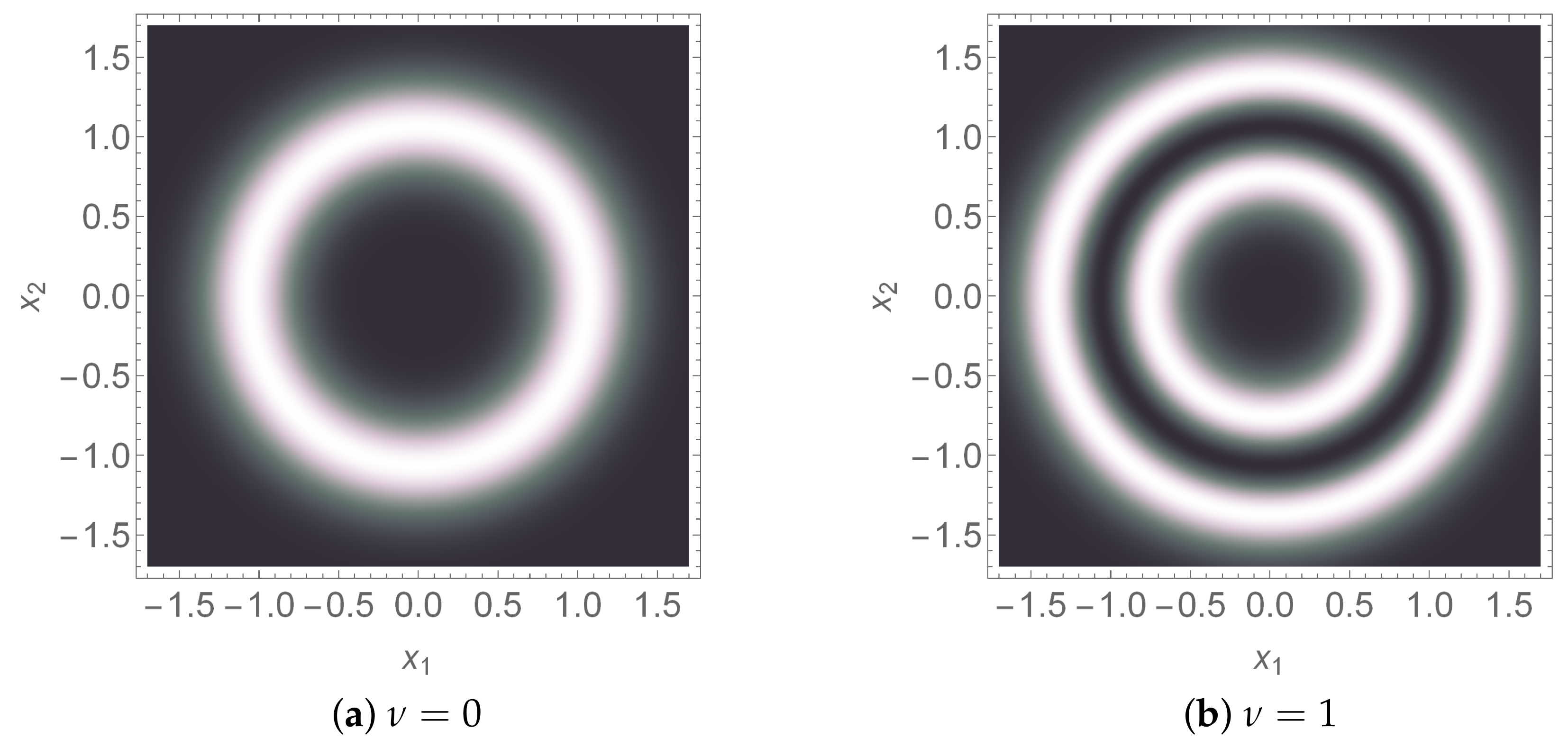
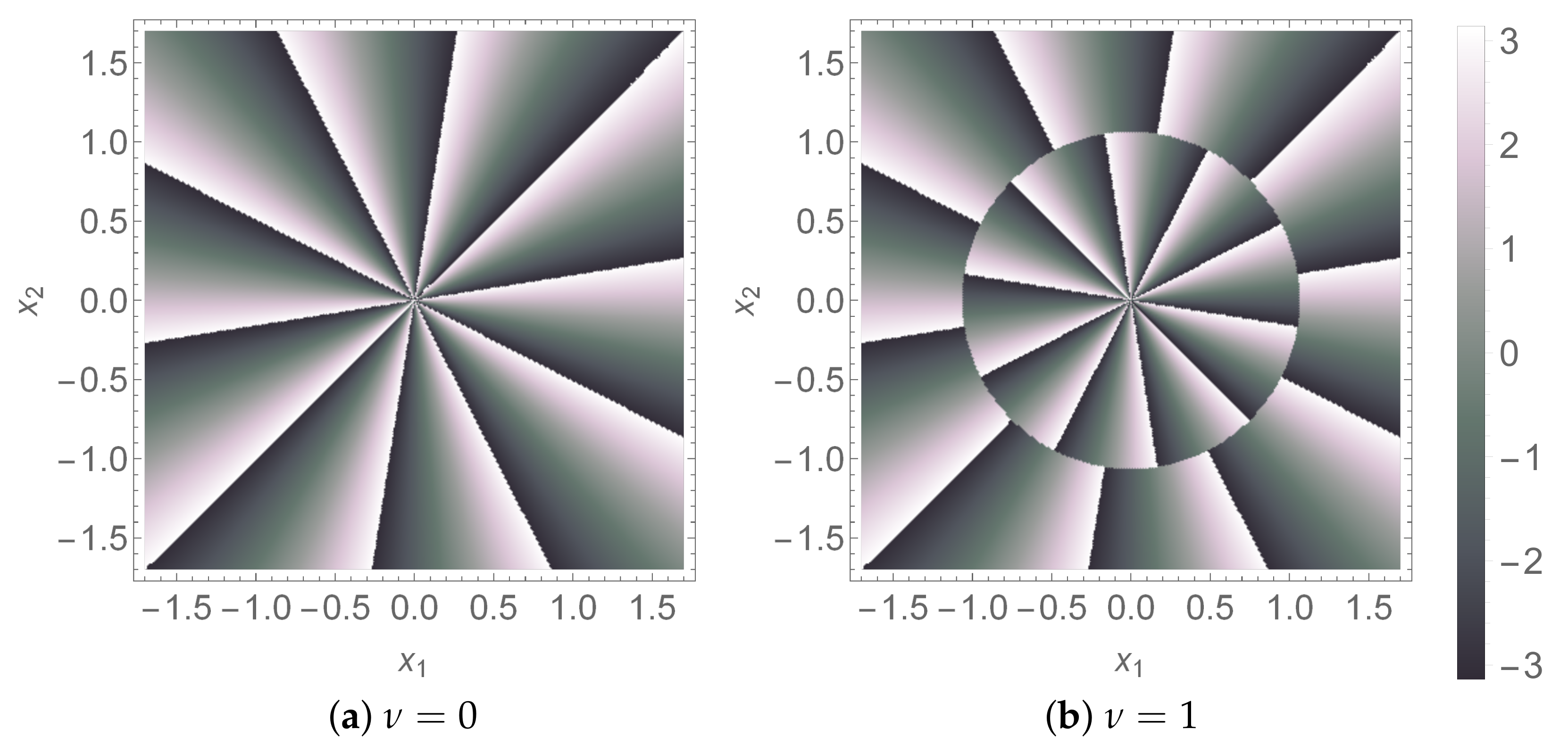
In Figure 2 and Figure 3, the plots of $|{\psi }_{\nu }\left(\overrightarrow{x}\right){|}^2$ and $\mathrm{Arg}\left[{\psi }_{\nu }\left(\overrightarrow{x}\right)\right]$ are shown for $\nu =0$ (56) and $\nu =1$ (57) when $\gamma =1$, $\varkappa =1$, $\hslash =0.1$, and $l=10$ (it corresponds to $\omega \approx 0.883$, $R\approx 1.06$, $\theta \approx 0.528$).

The phase incursion of $20\pi$ along the localization curve (Figure 2 and Figure 3) indicates that we have the vortex solution that corresponds to the solutions of the GPE with 10 quantum vortices [48]. However, since we construct asymptotics only in the neighborhood of the circumference, it do not allows us to obtain the complete information about the phase features in the center.

6. Conclusions

We applied the method proposed in [25] to constructing the solutions of the spectral problem for the stationary nonlocal GPE (7). The considered equation has rather general form with the limitation of the smoothness of the kernel of the nonlocal nonlinearity and of the symbol of the linear part. The solutions of the spectral problem were obtained by choosing the special solutions of the non-stationary nonlocal GPE semiclassically concentrated on time-invariant curves. Such solutions are found in terms of periodic solutions of the second order Hamilton–Ehrenfest system (A2) and (A5) and the set of linear independent skew-orthogonal Floquet solutions of the variational system (37).

The generalization of the method [25] for the stationary GPE is based on the following ideas. The time independence of the Equation (8) operator yields the symmetry (33) with respect to the t- and s-shift for the Equation (12) if the system (34) admits periodic solutions. The property (33) provides to the same symmetry for the second order Hamilton–Ehrenfest system, which leads to the Equations (A2) and (A5), and to the periodicity of coefficients in the variational system (23), that allows us to pose the Floquet problem for (37). Then, the periodic solutions of (A2) yield the symmetry for the associated linear GPE (18) and (20) that effectively reduces the number of independent variables in (18) from $(n+2)$ (n variables $\overrightarrow{x}$, t, and s) to $(n+1)$ (n variables $\overrightarrow{x}$, and $(t+s/\omega )$). This symmetry together with the Floquet solutions of (37) allows us to obtain the particular solutions (40) and (41) of the associated linear GPE (18) and (20) that give the solutions (42) of the stationary GPE (7) subject to the quantization conditions (48).

The feature of our method is that we do not reduce the initial n-dimensional problem to the one-dimensional. It means that, in general, our approach does not require the GPE to have some special symmetries. Nevertheless, various concepts of symmetries may be required for analytical integration of the auxiliary Equations (34), (37) and (A5) (e.g., [49]).

The solution constructed for the simplest form of the external field reminds the giant hole solution that was studied in [50]. It is known that vortices in the BEC are quantized so that each vortex corresponds to the phase incursion of $2\pi$ (see, e.g., [48]). The giant hole solutions are characterized by the proximity of vortex centres so that they form one density pit of the BEC [50] like our example. The indistinguishability of the vortex centres is the consequence of the semiclassical approximation. The centres of vortices likely can be identified within our approach by the consideration of a less trivial localization curve that is an open problem.

The solutions obtained here within the semiclassical approach proposed have the limit $\varkappa =0$ (the linear case) and decrease rapidly (exponentially) with distance from the localization curve. In the sense of these properties, the solutions of the nonlocal GPE correspond to ones studied in [11] for the one-dimensional local GPE. However, although the solutions localized on a curve cannot be directly reduced to the one-dimensional solutions found in [11], they explicitly reflect topological features of the BEC.

Note that the numerical calculations for the local and nonlocal GPEs show that, for the delta-like interaction kernel, the solutions of these type weakly change with an increase in the nonlocality coefficient $\gamma$, and qualitatively do not differ from the solutions of the local GPE when $\gamma$ is small. The solution is sensitive to the variation of $\gamma$ when the localization domain of the interaction potential becomes larger than the localization area of the BEC density. It caused by the sharp decrease in the interaction energy. Therefore, the nonlocal GPE can be treated not only as a separate problem but as the deformation of the local GPE for using our approach.

References

Pitaevskii, L.; Stringari, S. Bose–Einstein Condensation and Superfluidity; Oxford University Press: Oxford, UK, 2016. [Google Scholar]
Dalfovo, F.; Giorgini, S.; Pitaevskii, L.P.; Stringari, S. Theory of Bose–Einstein condensation in trapped gases. Rev. Mod. Phys.1999, 71, 463–512. [Google Scholar] [CrossRef] [Green Version]
Kevrekidis, P.G.; Frantzeskakis, D.J.; Carretero-Gonzalez, R. (Eds.) Emergent Nonlinear Phenomena in Bose–Einstein Condensates: Theory and Experiment; Springer: Berlin/Heidelberg, Germany, 2008. [Google Scholar]
Kevrekidis, P.G.; Frantzeskakis, D.J.; Carretero-Gonzales, R. The Defocusing Nonlinear Schrödinger Equation: From Dark Solitons to Vortices and Vortex Rings; SIAM: Philadelphia, PA, USA, 2015. [Google Scholar]
Baranov, M.A. Theoretical progress in many-body physics with ultracold dipolar gases. Phys. Rep.2008, 464, 71–111. [Google Scholar] [CrossRef]
Lahaye, T.; Menotti, C.; Santos, L.; Lewenstein, M.; Pfau, T. The physics of dipolar bosonic quantum gases. Rep. Prog. Phys.2009, 72, 126401. [Google Scholar] [CrossRef]
Beaufils, Q.; Chicireanu, R.; Zanon, T.; Laburthe-Tolra, B.; Maréchal, E.; Vernac, L.; Keller, J.; Gorceix, O. All-optical production of chromium Bose–Einstein condensates. Phys. Rev. A At. Mol. Opt. Phys.2008, 77, 061601. [Google Scholar] [CrossRef] [Green Version]
Jackson, A.D.; Kavoulakis, G.M.; Pethick, C.J. Solitary waves in clouds of Bose–Einstein condensed atoms. Phys. Rev. A At. Mol. Opt. Phys.1998, 58, 2417–2422. [Google Scholar] [CrossRef] [Green Version]
Pethick, C.J.; Smith, H. Bose–Einstein Condensation in Dilute Gases; Cambridge University Press: Cambridge, UK, 2008; pp. 1–569. [Google Scholar]
D’Agosta, R.; Malomed, B.A.; Presilla, C. Stationary solutions of the Gross–Pitaevskii equation with linear counterpart. Phys. Lett. Sect. A Gen. At. Solid State Phys.2000, 275, 424–434. [Google Scholar] [CrossRef] [Green Version]
D’Agosta, R.; Presilla, C. States without a linear counterpart in Bose–Einstein condensates. Phys. Rev. A At. Mol. Opt. Phys.2002, 65, 436091–436097. [Google Scholar] [CrossRef] [Green Version]
Antoine, X.; Duboscq, R. GPELab, a Matlab toolbox to solve Gross–Pitaevskii equations I: Computation of stationary solutions. Comput. Phys. Commun.2014, 185, 2969–2991. [Google Scholar] [CrossRef]
Bao, W.; Du, Q. Computing the ground state solution of Bose–Einstein condensates by a normalized gradient flow. SIAM J. Sci. Comput.2004, 25, 1674–1697. [Google Scholar] [CrossRef] [Green Version]
Bao, W.; Tang, W. Ground-state solution of Bose–Einstein condensate by directly minimizing the energy functional. J. Comput. Phys.2003, 187, 230–254. [Google Scholar] [CrossRef] [Green Version]
Carr, L.D.; Clark, C.W.; Reinhardt, W.P. Stationary solutions of the one-dimensional nonlinear Schrodinger equation. I. Case of repulsive nonlinearity. Phys. Rev. A At. Mol. Opt. Phys.2000, 62, 063610. [Google Scholar] [CrossRef] [Green Version]
Carr, L.D.; Clark, C.W.; Reinhardt, W.P. Stationary solutions of the one-dimensional nonlinear Schrodinger equation. II. Case of attractive nonlinearity. Phys. Rev. A At. Mol. Opt. Phys.2000, 62, 063611. [Google Scholar] [CrossRef] [Green Version]
Alfimov, G.L.; Gegel, L.A.; Lebedev, M.E.; Malomed, B.A.; Zezyulin, D.A. Localized modes in the Gross–Pitaevskii equation with a parabolic trapping potential and a nonlinear lattice pseudopotential. Commun. Nonlinear Sci. Numer. Simul.2019, 66, 194–207. [Google Scholar] [CrossRef] [Green Version]
Mallory, K.; Van Gorder, R.A. Stationary solutions for the nonlinear Schrödinger equation modeling three-dimensional spherical Bose–Einstein condensates in general potentials. Phys. Rev. E Stat. Nonlinear Soft Matter Phys.2015, 92, 013201. [Google Scholar] [CrossRef] [PubMed] [Green Version]
Sacchetti, A. Solution to the double-well nonlinear Schrödinger equation with Stark-type external field. J. Phys. A Math. Theor.2015, 48, 035303. [Google Scholar] [CrossRef]
Maslov, V. Operational Methods; Mir Publishers: Moscow, Russia, 1976. [Google Scholar]
Maslov, V. The Complex WKB Method for Nonlinear Equations. I. Linear Theory; Birkhauser Verlag: Basel, Switzerland, 1994. [Google Scholar]
Belov, V.V.; Dobrokhotov, S.Y. Semiclassical maslov asymptotics with complex phases. I. General approach. Theor. Math. Phys.1992, 92, 843–868. [Google Scholar] [CrossRef]
Shapovalov, A.V.; Kulagin, A.E.; Trifonov, A.Y. The Gross–Pitaevskii equation with a nonlocal interaction in a semiclassical approximation on a curve. Symmetry2020, 12, 201. [Google Scholar] [CrossRef] [Green Version]
Maslov, V. Complex Markov Chains and the Feynman Path Integral; Nauka: Moscow, Russia, 1976. [Google Scholar]
Maslov, V. Equations of the self-consistent field. J. Sov. Math.1978, 11, 123–195. [Google Scholar] [CrossRef]
Karasev, M.V.; Maslov, V.P. Algebras with general commutation relations and their applications. II. Unitary-nonlinear operator equations. J. Sov. Math.1981, 15, 273–368. [Google Scholar] [CrossRef]
Belov, V.V.; Kondrat’eva, M.F.; Smirnova, E.I. Semiclassical soliton-type solutions of the Hartree equation. Dokl. Math.2007, 76, 775–779. [Google Scholar] [CrossRef]
Anikin, A.Y.; Dobrokhotov, S.Y.; Nazaikinskii, V.E.; Tsvetkova, A.V. Uniform Asymptotic Solution in the Form of an Airy Function for Semiclassical Bound States in One-Dimensional and Radially Symmetric Problems. Theor. Math. Phys. Russ. Fed.2019, 201, 1742–1770. [Google Scholar] [CrossRef]
Shapovalov, A.V.; Rezaev, R.O.; Trifonov, A.Y. Symmetry operators for the Fokker-Plank-Kolmogorov equation with nonlocal quadratic nonlinearity. Symmetry Integr. Geom. Methods Appl. SIGMA2007, 3, 5. [Google Scholar] [CrossRef] [Green Version]
Levchenko, E.A.; Shapovalov, A.V.; Trifonov, A.Y. Asymptotics semiclassically concentrated on curves for the nonlocal Fisher-Kolmogorov-Petrovskii-Piskunov equation. J. Phys. A Math. Theor.2016, 49, 305203. [Google Scholar] [CrossRef]
Levchenko, E.A.; Shapovalov, A.V.; Trifonov, A.Y. Pattern formation in terms of semiclassically limited distribution on lower dimensional manifolds for the nonlocal Fisher-Kolmogorov-Petrovskii-Piskunov equation. J. Phys. A Math. Theor.2014, 47, 025209. [Google Scholar] [CrossRef] [Green Version]
Pereskokov, A.V. Semiclassical asymptotics of the spectrum near the lower boundary of spectral clusters for a Hartree-type operator. Math. Notes2017, 101, 1009–1022. [Google Scholar] [CrossRef]
Pereskokov, A.V. Asymptotics of the Spectrum of a Two-dimensional Hartree Type Operator Near Upper Boundaries of Spectral Clusters. Asymptotic Solutions Located Near a Circle. J. Math. Sci.2017, 226, 517–530. [Google Scholar] [CrossRef]
Lugiato, L.A.; Lefever, R. Spatial dissipative structures in passive optical systems. Phys. Rev. Lett.1987, 58, 2209–2211. [Google Scholar] [CrossRef] [PubMed]
Chembo, Y.K.; Menyuk, C.R. Spatiotemporal Lugiato-Lefever formalism for Kerr-comb generation in whispering-gallery-mode resonators. Phys. Rev. A At. Mol. Opt. Phys.2013, 87, 053852. [Google Scholar] [CrossRef] [Green Version]
Coen, S.; Randle, H.G.; Sylvestre, T.; Erkintalo, M. Modeling of octave-spanning Kerr frequency combs using a generalized mean-field Lugiato-Lefever model. Opt. Lett.2013, 38, 37–39. [Google Scholar] [CrossRef] [PubMed] [Green Version]
Godey, C.; Balakireva, I.V.; Coillet, A.; Chembo, Y.K. Stability analysis of the spatiotemporal Lugiato-Lefever model for Kerr optical frequency combs in the anomalous and normal dispersion regimes. Phys. Rev. A At. Mol. Opt. Phys.2014, 89, 063814. [Google Scholar] [CrossRef] [Green Version]
Butov, L.V.; Lai, C.W.; Ivanov, A.L.; Gossard, A.C.; Chemla, D.S. Towards Bose–Einstein condensation of excitons in potential traps. Nature2002, 417, 47–52. [Google Scholar] [CrossRef] [PubMed]
Sob’Yanin, D.N. Bose–Einstein condensation of light: General theory. Phys. Rev. E Stat. Nonlinear Soft Matter Phys.2013, 88, 022132. [Google Scholar] [CrossRef] [Green Version]
Berman, O.L.; Kezerashvili, R.Y. Superfluidity of dipolar excitons in a transition metal dichalcogenide double layer. Phys. Rev. B2017, 96, 094502. [Google Scholar] [CrossRef] [Green Version]
Berman, O.L.; Gumbs, G.; Kezerashvili, R.Y. Bose–Einstein condensation and superfluidity of dipolar excitons in a phosphorene double layer. Phys. Rev. B2017, 96, 014505. [Google Scholar] [CrossRef] [Green Version]
Elizalde, E.; Lidsey, J.E.; Nojiri, S.; Odintsov, S.D. Born-Infeld quantum condensate as dark energy in the universe. Phys. Lett. Sect. B Nucl. Elem. Part. High Energy Phys.2003, 574, 1–7. [Google Scholar] [CrossRef] [Green Version]
Addazi, A.; Capozziello, S.; Odintsov, S. Born–Infeld condensate as a possible origin of neutrino masses and dark energy. Phys. Lett. Sect. B Nucl. Elem. Part. High Energy Phys.2016, 760, 611–616. [Google Scholar] [CrossRef] [Green Version]
Bagrov, V.G.; Belov, V.V.; Trifonov, A.Y. Semiclassical trajectory-coherent approximation in quantum mechanics I. High-order corrections to multidimensional time-dependent equations of Schrödinger type. Ann. Phys.1996, 246, 231–290. [Google Scholar] [CrossRef]
Fetter, A.L.; Svidzinsky, A.A. Vortices in a trapped dilute Bose–Einstein condensate. J. Phys. Condens. Matter2001, 13, R135–R194. [Google Scholar] [CrossRef] [Green Version]
Obukhov, V.V. Algebra of symmetry operators for Klein-Gordon-Fock equation. Symmetry2021, 13, 727. [Google Scholar] [CrossRef]
Kasamatsu, K.; Tsubota, M.; Ueda, M. Giant hole and circular superflow in a fast rotating Bose–Einstein condensate. Phys. Rev. A At. Mol. Opt. Phys.2002, 66, 053606. [Google Scholar] [CrossRef] [Green Version]
Figure 1.
The values of for various quantum numbers l and for , (black), , (red), , (blue).
Figure 2.
Density plots of .
Figure 3.
Publisher’s Note: MDPI stays neutral with regard to jurisdictional claims in published maps and institutional affiliations.
Kulagin, A.E.; Shapovalov, A.V.; Trifonov, A.Y.