Abstract
Fuzzy graphs (FGs), broadly known as fuzzy incidence graphs (FIGs), are an applicable and well-organized tool to epitomize and resolve multiple real-world problems in which ambiguous data and information are essential. In this article, we extend the idea of domination of FGs to the FIG using strong pairs. An idea of strong pair dominating set and a strong pair domination number (SPDN) is explained with various examples. A theorem to compute SPDN for a complete fuzzy incidence graph (CFIG) is also provided. It is also proved that in any fuzzy incidence cycle (FIC) with l vertices the minimum number of elements in a strong pair dominating set are . We define the joining of two FIGs and present a way to compute SPDN in the join of FIGs. A theorem to calculate SPDN in the joining of two strong fuzzy incidence graphs is also provided. An innovative idea of accurate domination of FIGs is also proposed. Some instrumental and useful results of accurate domination for FIC are also obtained. In the end, a real-life application of SPDN to find which country/countries has/have the best trade policies among different countries is examined. Our proposed method is symmetrical to the optimization.
1. Introduction
A graph is an easy way to express information, together with the relationship between various kinds of entities. The entities are indicated by vertices and relations are illustrated by edges. In this paper, we use finite and simple graphs. A mathematical framework to explain inconclusiveness and ambiguity in real-life situations was first recommended by Zadeh. He initiated the idea of Fuzzy set (FS) [1,2]. When there is an inadequacy in the explanation of the objects and their relationship, we need to draw a FG model. Zadeh’s FS prepares a way for the theory of FGs which has been contemplated by Rosenfeld [3]. The study of FGs opens a new door for many researchers to participate in this field. For instance, Gani and Ahamed [4] presented an idea to find order and size in FGs. Bhutani et al. [5] discussed degrees for fuzzy end nodes and studied some properties of fuzzy end nodes and fuzzy cut nodes further. The notion of domination in FGs was first suggested by Somasundaram and Somasundaram [6]. Later, Somasundaram [7] discussed domination in products of FGs. Gani and Ahamed [8] initiated the notion of strong and weak domination in FGs along with their different properties. Natarajan and Ayyaswamy [9] initiated the idea of strong (weak) domination in FGs and obtained some interesting results for this new parameter in FGs. Various types of degrees of a node in FGs were introduced by Manjusha and Sunitha [10]. They obtained the lower and upper bound of domination number for the FGs and also proved that in a fuzzy tree each node of a dominating set is incident on a fuzzy bridge. Manjusha and Sunitha [11] introduced the idea of total domination in FGs using strong arcs and discussed a lower bound and an upper bound for the strong total domination number in FGs. They also presented the necessary and sufficient condition for the set of fuzzy cut nodes to be a strong total dominating set. The strong domination number of complete FG and complete bipartite FG was introduced by Manjusha and Sunitha [12]. After them, the equitable dominating set, minimal fuzzy equitable dominating set, strong (weak) fuzzy equitable dominating set, and fuzzy equitable independent set in FGs were discussed by Dharmalingam and Rani [13]. Then, 2-domination in FGs was introduced by Gani and Devi [14]. Gani and Rahman [15] proposed an innovative idea of an accurate 2-dominating set and accurate 2-domination number of a FG. They also elaborated some properties of accurate 2-dominating sets and also some bounds of accurate 2-domination numbers. Ponnappan et al. [16] brought the notion of edge domination and total edge domination in FGs. They determined the edge domination number and the total edge domination number for several classes of FG and obtained bounds for the same. The concept of very excellent domination in FGs along with their various properties was proposed by Nithya and Dharmalingam [17].
Bhutani and Rosenfeld [18] came up with an idea of strong arcs in FGs. Mathew and Mordeson [19] presented the novel idea of fuzzy influence graph and characterized influence cutpairs in fuzzy influence graphs since their removal increases the number of connected components of a fuzzy network and thus weakens the potential flow in the network. They also discussed some of the properties of influence pairs and influence cut-nodes. Rashmanlou and Jun [20] defined three new operations on interval-valued FGs; namely, direct product, semi-strong product, and strong product. Likewise, they gave sufficient conditions for each one of them to be complete and show that if any of these products is complete, then at least one factor is a complete interval-valued FG. The idea of a complement of an FG was initiated by Sunitha and Vijayakumar [21]. Yin et. al [22] introduced the degree of a vertex the degree and total degree of a vertex in q-rung orthopair FGs. They also found some product operations on q-rung orthopair FGs, including direct product, Cartesian product, semi-strong product, strong product, and lexicographic product. For some other useful and constructive work on FGs, we suggest to the reader [23,24,25,26,27].
FGs are incapable of intimating the impact of a vertex on an edge.This deficiency in FGs became the main reason to introduce the idea of FIGs. Dinesh [28] was the first researcher who introduced the concept of FIGs. For example, if vertices represent various hospitals and edges serve as roads connecting these hospitals, we can have an FG indicating the extent of traffic from one hospital to another hospital. The hospital having the highest number of patients will have the most ramps in the hospital. So, if L and M are two hospitals and LM is a road connecting them then (L, LM) can present the ramp system from the road LM to the hospital L. In unweighted graphs, both L and M will have an impact of 1 on LM. In a directed graph, the influence of L on LM given by (L, LM) is 1 whereas (M, LM) is 0. This idea can be generalized by FIGs. Malik et al. [29] provided initial results to the development a final area of -fuzzy type incidence graphs, namely -fuzzy incidence for complementary FIGs. They applied the results to problems involving human trafficking. They were particularly interested in the role played by countries’ vulnerability and their government’s response to human trafficking. Mathew and Mordeson [30] presented various connectivity concepts in FIGs. They established the existence of a strong path between any node arc pair of a FIG. They also discussed several other structural properties of FIGs. Fang et al. [31] presented the idea of connectivity index and Wiener index of FIGs. They also introduced three different types of nodes including fuzzy incidence connectivity enhancing node, fuzzy incidence connectivity reducing node, and fuzzy incidence connectivity neutral node. After them, Mathew et al. [32] presented the notion of node connectivity and arc connectivity in FIGs. They also discussed that the incidence is used to model flows in human trafficking networks. The conception of fuzzy end nodes and relationships among weak incidence pairs, fuzzy incidence end nodes, and fuzzy incidence cutvertices was developed by Mordeson and Mathew [33]. Later, Nazeer et al. [34] introduced intuitionistic fuzzy incidence graphs (IFIGs) as a generalization of FIGs and explained various types of products including Cartesian product (CP), composition, tensor product, and normal product in IFIGs. They also provided an application of CP and composition of two IFIGs in the textile industry to find the best combinations of departments indicating the highest percentage of progress and the lowest percentage of non-progress. Nazeer et al. [35] came up with an innovative idea of domination in FIGs along with an algorithm and an application for the selection of the best medical lab among a variety of labs. Mordeson et al. [36] introduced the notion of a vague incidence graph and its eccentricity. They applied the results to problems involving human trafficking and illegal immigration. For more detailed and comprehensive work on FIGs, we may refer to the reader [28,37].
There are multiple reasons to initiate the idea of domination in the joining of FIGs using strong pairs (SPs). Firstly, we are unable to apply FGs to the real-life application provided in Section 6 of SPDN in matters of trade of different countries because FGs do not have a feature to give the impact of a vertex on an edge but FIGs have this property. This deficiency of FGs motivates us to introduce these ideas for FIGs. Secondly, the purpose to propose these perceptions to FIGs is that Selvam and Ponnappan [38] proposed the idea of domination in the join of FGs using strong edges (SEs), and Ponnappan and Selvam [39] came up with the idea of accurate domination in FGs using SEs. We broaden their ideas for FIGs by using SPs. Thirdly, in FGs if an edge uv is a SE then vu will also be a SE but in FIG if a pair (u,uv) is a SP then the pair (v,uv) don’t need to be a SP. It may or may not be a SP. Fourthly, in FGs if a vertex u dominates vertex v then vertex v will also dominate a vertex u but in FIGs, if a vertex u dominates a vertex v then it is not necessary that a vertex v will also dominate a vertex u because in FIGs if a pair (u,uv) is a SP then a pair (v,uv) may or may not be a SP.
The remainder of this article is organized as follows. In Section 2, some fundamental definitions and preliminary results which are helpful to comprehend the remaining part of the article are explained with various examples. The domination in FIGs using SPs and some significant results are expressed in Section 3. In Section 4, domination in the joining of FIGs is elaborated. Section 5 provides the information of accurate domination in FIGs. A real-life application of domination in matters of trading among different countries is explained in Section 6. A comparative analysis of our study with the previous study is provided in Section 7. Conclusions and future directions are explained in Section 8.
2. Preliminaries
We recall some fundamental definitions in FIGs and propose some novel definitions and ideas. We present some preliminary definitions from [1,30,38] in the following sections. In this article, the minimum and maximum operators are indicated by ∧ and ∨, respectively.
Definition 1
([38]). A FG is a pair of function and where for each , we have .
Definition 2
([38]). A path ϖ of length n in a FG is a sequence of different vertices of the type where . Vertices s and t in a FG are called to be connected if ∃ path in . In a FG if s and t are connected by means of length i, then .
Definition 3
([38]). The strongest path (SGP) joining any two vertices s and t is a path corresponding to greatest strength between s and t. The strength of the SGP is expressed by . Where .
Example 1.
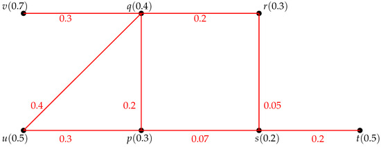
Figure 1 indicates a FG with . In this FG there are four paths from u to r namely, path of length 2 and strength , path of length 4 and strength , path of length 3 and strength and path of length 3 and strength . The strength of the SGP joining u and r is .
Figure 1.
FG with strongest path.
Definition 4
([38]). An edge of a FG is said be SE if .
Definition 5
([38]). Let be a FG. Assume s and t are any two vertices of a FG. A vertex s dominates t if the edge is SE. A subset Z of V is said to be a strong edge dominating set (SEDS) of FG if for each such that s dominates t. A SEDS Z is named as a minimal SEDS if no proper subset of Z is a SEDS. The minimum fuzzy cardinality (MFC) taken over all minimal SEDS is said to be strong edge domination number (SEDN), indicated by .
Definition 6
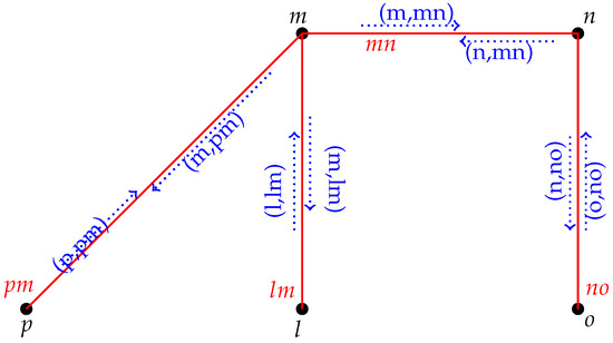
([30]). Let G be a simple graph with vertex set and edge set . is called an incidence graph (IG) where . Figure 2 shows an IG.
Figure 2.
Incidence graph.
If is in IG, then is said to be an incidence pair or pair of an IG.
Definition 7
([1]). If T is any set, a mapping is known as fuzzy subset (FSS) of S.
Definition 8
([30]). Assume is a graph with σ is FSS of V, ϕ is FSS of E and η is FSS of . If and , then η is named as fuzzy incidence (FI) of G.
Definition 9
([30]). Consider is a graph and be a fuzzy subgraph of G. If η is a FI of G, then is named as FIG of G.
Definition 10
([30]). Any is said to be in the support of σ if , is said to be in the support of ϕ if and is said to be in the support of η if . The support of and η are expressed by , , and , respectively. Let . Then is an edge of the FIG and if then is called pair of FIG. In FIG is an incidence path (IP) of length one, is an IP of length two. In a FIG two vertices and are said to be connected if they are joined by an IP. and are two different types of IPs in FIG. The incidence strength (IS) of a FIG is defined as .
Definition 11
([30]). The FIG is a cycle if is a cycle. The FIG is a fuzzy cycle if is a cycle and there exists no unique such that . The FIG is a fuzzy incidence cycle (FIC), and there exists no unique such that .
A FIC is shown in Figure 3.
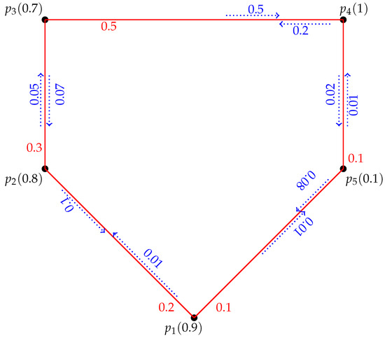
Figure 3.
Fuzzy incidence cycle.
Proposition 1
([30]). Every FIC is a strong cycle.
Definition 12
([30]). A FIG is said to be complete FIG if for every .
3. Domination in Fuzzy Incidence Graph Using Strong Pair
Domination in graphs has plenty of uses in various fields. The idea of domination using SPs with various examples is explained in this section. An idea of strong pair dominating set (SPDS) and SPDN is discussed. In the future these concepts will be helpful to find SPDS and SPDN in various types of products of FIGs.
Definition 13.
Let be a FIG. An edge in FIG is called an effective edge if .
Definition 14.
A pair in FIG is called an effective pair (EP) if .
Definition 15.
Let be a FIG. The IS of an IP between the vertex s and an edge is defined as IS.
Definition 16.
Assume is a FIG. If a vertex s and an edge in a FIG are connected by means of length w, then .
Definition 17.
Consider is a FIG. The greatest incidence strength (GIS) between s and is the largest value of all ISs of all IPs between s and and it is represented by .
Example 2.
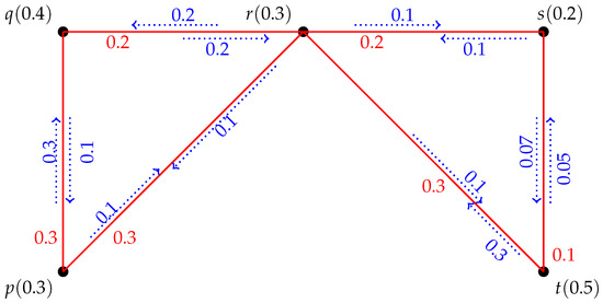
Figure 4 indicates a FIG with . In this FIG there are two IPs from p to of length 1 and length 4, respectively, namely, with IS and having IS. The GIS between p and is .
Figure 4.
FIG with strong and non strong pairs.
Definition 18.
Assume a FIG . A pair is called SP if otherwise it is not strong.
Example 3.
Figure 4 represents a FIG with . In this FIG there are two IPs from p to namely, with IS and having IS. Therefore, is a SP because .
Definition 19.
Let be a FIG. Let s and t be any two vertices of . A vertex s dominates t if is a SP. A subset Z of V is named as a SPDS of if for each such that s dominates t.
Definition 20.
Let be a FIG. Then a SPDS Z is named as minimal SPDS if no proper subset of Z is a SPDS.
Definition 21.
Consider is a FIG. Then the MFC taken over all minimal SPDS is said to be SPDN, represented by or .
Definition 22.
Let be a FIG. Then the lowest number of elements in the minimal SPDS is expressed by where is a minimal SPDS.
Example 4.
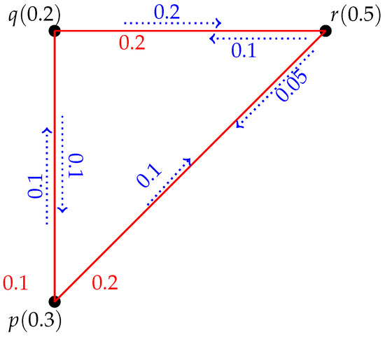
A FIG is provided in Figure 5 with . In this FIG and are all SPs. Therefore, there are two minimal SPDSs which are because p dominates q and r and because q dominates p and r. This implies because has the lowest fuzzy cardinality.
Figure 5.
FIG with .
Theorem 1.
A pair (s,st) in FIG is a SP if and only if there does not exist an IP of the kind for each .
Proof.
Let be a SP. Assume ∃ an IP of the type for each . Then GIS of . This means . Therefore, is not SP which is a contradiction. Consider there does not exist an IP such that for every . This implies that for each IP of a pair of the type for some j. This implies for each IP of , GIS of . This implies . Hence is a SP. □
Example 5.
Let be a FIG shown in Figure 4 with . In this FIG there are two IPs from p to namely, with and having and . Therefore, according to Theorem 1 is a SP because there does not exist any pair of the type such that , , , and .
Definition 23.
Consider s is a vertex in a FIG . We define where is the highest weights of the pairs incidence at s.
Theorem 2.
Let be a FIG and consider is a pair in FIG such that then is a SP.
Proof.
Assume is not a SP then there exists an IP such that GIS of . This means for every . This implies which is a contradiction. □
Example 6.
Consider a FIG provided in Figure 5 with . In this FIG is a SP because .
Theorem 3.
Let be a FIG. If is an EP then it must be a SP.
Proof.
Assume is an EP. Then . Suppose . Then . Therefore, for any IP , GIS of and . This implies . Therefore, is a SP. □
Example 7.
Theorem 4.
Let be a CFIG then .
Proof.
Assume Z is a dominating set. Consider and . Since is a therefore every pair is an EP. Then by Theorem 4 each pair is also a SP. Therefore, s dominates every . This means is a SPDS. Hence . □
Example 8.
Let be a with . Since is a therefore each pair is an EP. Therefore, by Theorem 3 every pair is also a SP. This means that each vertex dominates to another vertex i.e. p dominates q and r, q dominates p and r, and r dominates p and q. Now , and are all SPDSs. Therefore, . Hence Theorem 4 is verified.
Theorem 5.
Let be a FIC with l vertices then .
Proof.
Let be a FIC then by Proposition 1 every FIC is a strong cycle therefore each pair in is SP. Therefore, every vertex of can dominate up to two other vertices and itself. Taking each third vertex beginning from the second and utilizing the end when l is indivisible by three yields a minimal SPDS of size . This implies . □
Example 9.
Let be a FIC with five vertices given in Figure 3 with . Since is a FIC and by Proposition 1 each pair in a FIC is a SP. Therefore, according to Example 6 which are , , , and .
4. Domination in the Join of Fuzzy Incidence Graphs
In this section, some new ideas of domination along with various examples are explained. The method to find join of two FIGs is provided in this section. The definition of strong fuzzy incidence graph is also obtained in this section. The join of two SFIGs is always SFIG is also elaborated in this section.
Definition 24.
Let and be two FIGs. The join of and is expressed by and is defined as the FIG where
and
Definition 25.
A FIG is called a if every pair in is strong.
Theorem 6.
Let and be two SFIGs. Then where and .
Proof.
Assume and are two SFIGs. Since and are two SFIGs then will also a SFIG. So, each vertex in will dominates other vertices. Then by definition of SPDN, . □
Theorem 7.
Let and be two SFIGs with and , where e and f are representing the number of vertices in and , respectively. Then .
Proof.
Consider and are two SFIGs. Let and be SPDSs of and , respectively. Since and are SFIGs. Then will also a SFIG with because one vertex in dominates to all remaining vertices. □
5. Accurate Domination in Fuzzy Incidence Graphs
An innovative idea of accurate domination in FIG is proposed in this section. Some meaningful results related to accurate domination are also examined. Some useful results of accurate domination for FIC are elaborated.
Definition 26.
A SPDS Z of a FIG is named as accurate dominating set (ADS) if V-Z has no SPDS of cardinality .
Definition 27.
Let be a FIG. Then the accurate domination number (ADN) of is the lowest cardinality of an ADS and it is represented by .
Example 11.
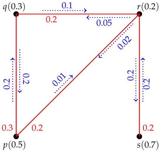
Figure 9 shows a FIG with . In all pairs are strong except and an ADS with .
Figure 9.
FIG with .
Theorem 8.
Let be a FIC, then , where and .
Proof.
Assume are the vertices of . By definition of FIC every pair in FIC is SP. Let Z be the minimum of . Therefore, every vertex absolutely dominates two vertices in . By Definition 23 . Therefore, Z is an ADS with . □
Theorem 9.
Let be a FIC, then , where and .
Proof.
Consider are the vertices of . Since is a FIC then by definition of FIC each pair is SP. So, each vertex dominates to vertices and . Assume Z is the minimum SPDS of . Then by Definition 23 . This implies Z is an ADS with . □
Theorem 10.
Let be a FIC, then , where and .
Proof.
Consider are the vertices of . Since is a FIC then by definition of FIC each pair is SP. So, each vertex dominates to vertices and . Let Z be the minimum SPDS of . Then by Definition 23 . This implies Z is an ADS with . □
6. Real-Life Application of Strong Pair Domination Number
Here we include a real-life application of SPDN in matters of trade among different countries. As an illustrative case, consider a network (FIG) of six vertices representing six different countries , and as shown in Figure 10. The membership value (MSV) of the vertices shows the population of the country. The MSV of the edges represents the relationship among these countries and the MSV of the pairs denotes the best trade policies among these countries. The investors are interested in investing their money in these countries but, before they invest, they want to know which country/countries has/have the best trade policies. With the help of SPDN, we will be able to find which country/countries has/have the best trade policies. In turn, this knowledge would help them tackle any risk in their investment.
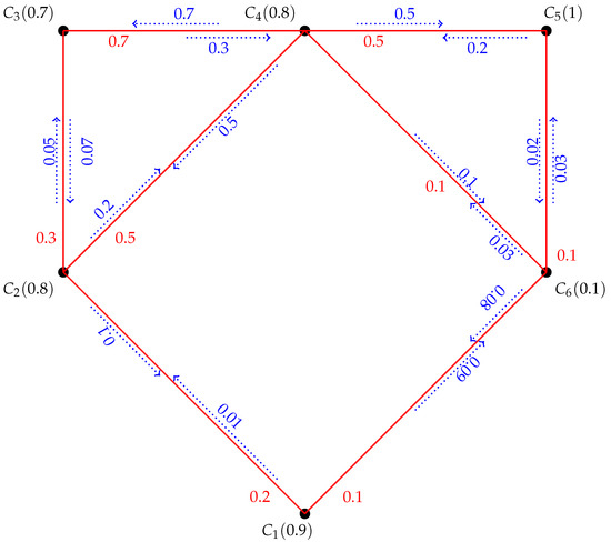
Figure 10.
A graphical model representing trade among different countries.
In Figure 10, is SP because . Similarly, and are all SPs. Also, . Therefore, is not SP. In similar way, and are not SPs. The SPDSs are with and . So, investors can invest in country and because these two countries have best trade policies among all other countries.
7. Comparative Analysis
In Figure 10, a FIG indicating six different countries , and . The MSV of the vertices representing the inhabitants of the country, the MSV of the edges expressing the relationship among these countries and the MSV of the pairs represent the best trade policies among these countries. In the case of FIG we get SPDS with . But in Figure 10, if we remove all the pairs we get a FG. In the case of FG, we find all strong and non SEs. First we check is a SE or not. In Figure 10 it can be seen that there are five possible paths from to which are is a path of length 1 with strength . is a path of length 4 with strength . is a path of length 5 with strength . is a path of length 3 with strength . is a path of length 4 with strength . The strength of the SGP joining and is is the largest value of all the strengths between and . Since therefore is a SE. In the same way, and are all SEs. But is not a SE because . All possible SEDSs of the FG are and with . Similarly, and . Now, it can be seen in Figure 10 that in case of FIG the set with has two countries which have best trade policies among all other countries but in the case of FG we are unable to talk about best trade policies due to non-availability of pairs. FGs can show the relationship among different countries but silent to talk about trade policies among different countries. Therefore, FIGs are more beneficial and effective than FGs.
8. Conclusions
The concept of domination in graphs is very rich both from a theoretical as well as applications point of view. Domination ideas in graphs are crucial from a different perspective. It has multiple uses in various fields of life. Different authors have investigated more than thirty domination parameters. In this article, we propose the novel idea of domination in FIGs using SPs. The notion of SPDS and SPDN for various types of FIGs with different examples is also explained. An idea of domination in the join of FIGs and accurate domination using SPs with a variety of examples in FIGs is presented in this article. Some significant results related to accurate domination are also investigated. Several handy and key results of accurate domination for FIC with different examples are also discussed. SPDN and ADN are introduced for different FIGs. SPDN for CFIGs is also explored with certain examples. Some beneficial and instrumental theorems of domination in the join of FIGs are also explained. An application of SPDN in matters of trade among different countries is accomplished too. In the future, we aim to extend our research work to Hamiltonian FIGs, the coloring of FIGs, and the chromaticity of FIGs. Further work on these ideas will be reported in upcoming papers.
Author Contributions
This paper is a result of common work of the authors in all aspects. Investigation, I.N., T.R. and M.T.H.; Writing—original draft, J.L.G.G. All authors have read and agreed to the published version of the manuscript.
Funding
Research work is partially supported by Ministerio de Ciencia, Innovación y Universidades grant number PGC2018-097198-B-I00 and Fundación Séneca. de la Región de Murcia grant number 20783/PI/18. Authors are thankful to the reviewers for their comments and suggestions to improve the quality of the manuscript.
Data Availability Statement
This work is not based on any data.
Conflicts of Interest
The authors declare no conflict of interest.
References
- Zadeh, L.A. Fuzzy sets. Inf. Control 1965, 8, 338–353. [Google Scholar] [CrossRef]
- Zadeh, L.A. Is there a need for fuzzy logic? Inf. Sci. 2008, 178, 2751–2779. [Google Scholar] [CrossRef]
- Rosenfeld, A. Fuzzy Graphs, Fuzzy Sets and Their Applications to Cognitive and Decision Processes; Elsevier: Amsterdam, The Netherlands, 1975; pp. 77–95. [Google Scholar]
- Gani, A.N.; Ahamed, M.B. Order and size in fuzzy graphs. Bull. Pure Appl. Sci. 2003, 22, 145–148. [Google Scholar]
- Bhutani, K.R.; Mordeson, J.; Rosenfeld, A. On degrees of end nodes and cut nodes in fuzzy graphs. Iran. J. Fuzzy Syst. 2004, 1, 57–64. [Google Scholar]
- Somasundaram, A.; Somasundaram, S. Domination in fuzzy graphs-I. Pattern Recognit. Lett. 1998, 19, 787–791. [Google Scholar] [CrossRef]
- Somasundaram, A. Domination in products of fuzzy graphs. Int. J. Uncertain. Fuzziness Knowl. Based Syst. 2005, 13, 195–204. [Google Scholar] [CrossRef]
- Gani, A.N.; Ahamed, M.B. Strong and weak domination in fuzzy graphs. East Asian Math. J. 2007, 23, 1–8. [Google Scholar]
- Natarajan, C.; Ayyaswamy, S. On strong (weak) domination in fuzzy graphs. Int. J. Math. Comput. Sci. 2010, 4, 1035–1037. [Google Scholar]
- Manjusha, O.; Sunitha, M. Notes on domination in fuzzy graphs. J. Intell. Fuzzy Syst. 2014, 27, 3205–3212. [Google Scholar] [CrossRef]
- Manjusha, O.; Sunitha, M. Total domination in fuzzy graphs using strong arcs. Ann. Pure Appl. Math. 2014, 9, 23–33. [Google Scholar]
- Manjusha, O.; Sunitha, M. Strong domination in fuzzy graphs. Fuzzy Inf. Eng. 2015, 7, 369–377. [Google Scholar] [CrossRef]
- Dharmalingam, K.; Rani, M. Equitable domination in fuzzy graphs. Int. J. Pure Appl. Math. 2014, 94, 661–667. [Google Scholar] [CrossRef][Green Version]
- Gani, A.N.; Devi, K.P. 2-domination in fuzzy graphs. Int. J. Fuzzy Math. Arch. 2015, 9, 119–124. [Google Scholar]
- Gani, A.N.; Rahman, A.A. Accurate 2-domination in fuzzy graphs using strong arcs. Int. J. Pure Appl. Math. 2018, 118, 279–286. [Google Scholar]
- Ponnappan, C.; Ahamed, S.B.; Surulinathan, P. Edge domination in fuzzy graphs new approach. Int. J. It Eng. Appl. Sci. Res. 2015, 4, 14–17. [Google Scholar]
- Nithya, P.; Dharmalingam, K. Very excellent domination in fuzzy grpahs. Int. J. Comput. Appl. Math. 2017, 12, 313–326. [Google Scholar]
- Bhutani, K.R.; Rosenfeld, A. Strong arcs in fuzzy graphs. Inf. Sci. 2003, 152, 319–322. [Google Scholar] [CrossRef]
- Mathew, S.; Mordeson, J.N. Fuzzy influence graphs. New Math. Nat. Comput. 2017, 13, 311–325. [Google Scholar] [CrossRef]
- Rashmanlou, H.; Jun, Y.B. Complete interval-valued fuzzy graphs. Ann. Fuzzy Math. Inform. 2013, 6, 677–687. [Google Scholar]
- Sunitha, M.; Vijayakumar, A. Complement of a fuzzy graph. Indian J. Pure Appl. Math. 2002, 33, 1451–1464. [Google Scholar]
- Yin, S.; Li, H.; Yang, Y. Product operations on q-rung orthopair fuzzy graphs. Symmetry 2019, 11, 588. [Google Scholar] [CrossRef]
- Mordeson, J.N.; Nair, P.S. Fuzzy graphs and fuzzy hypergraphs. Physica 2012, 46. [Google Scholar] [CrossRef]
- Bershtein, L.S.; Bozhenyuk, A.V. Fuzzy graphs and fuzzy hypergraphs. In Encyclopedia of Artificial Intelligence; IGI Global: Hershey, PA, USA, 2009; pp. 704–709. [Google Scholar] [CrossRef]
- Mathew, S.; Mordeson, J.N.; Malik, D.S. Fuzzy Graph Theory; Springer: Berlin/Heidelberg, Germany, 2018. [Google Scholar]
- Mordeson, J.N.; Chang-Shyh, P. Operations on fuzzy graphs. Inf. Sci. 1994, 79, 159–170. [Google Scholar] [CrossRef]
- Yeh, R.T.; Bang, S.Y. Fuzzy relations, fuzzy graphs, and their applications to culstering analysis. In Fuzzy Sets and Their Applications to Cognitive and Decision Processes; Elsevier: Amsterdam, The Netherlands, 1975; pp. 125–149. [Google Scholar]
- Dinesh, T. Fuzzy incidence graph—An introduction. Adv. Fuzzy Sets Syst. 2016, 21, 33–48. [Google Scholar] [CrossRef]
- Malik, D.S.; Mathew, S.; Mordeson, J.N. Fuzzy incidence graphs: Applications to human trafficking. Inf. Sci. 2018, 447, 244–255. [Google Scholar] [CrossRef]
- Mathew, S.; Mordeson, J.N. Connectivity concepts in fuzzy incidence graphs. Inf. Sci. 2017, 382–383, 326–333. [Google Scholar] [CrossRef]
- Fang, J.; Nazeer, I.; Rashid, T.; Liu, J.B. Connectivity and Wiener index of fuzzy incidence graphs. Math. Probl. Eng. 2021, 2021, 1–7. [Google Scholar] [CrossRef]
- Mathew, S.; Mordeson, J.N.; Yang, H.L. Incidence cuts and connectivity in fuzzy incidence graphs. Iran. J. Fuzzy Syst. 2019, 16, 31–43. [Google Scholar]
- Mordeson, J.N.; Mathew, S. Fuzzy end nodes in fuzzy incidence graphs. New Math. Nat. Comput. 2017, 13, 13–20. [Google Scholar] [CrossRef]
- Nazeer, I.; Rashid, T.; Keikha, A. An application of product of intuitionistic fuzzy incidence graphs in textile industry. Complexity 2021. [Google Scholar] [CrossRef]
- Nazeer, I.; Rashid, T.; Guirao, J.L.G. Domination of fuzzy incidence graphs with the algorithm and application for the selection of a medical lab. Math. Probl. Eng. 2021, 2021, 1–11. [Google Scholar] [CrossRef]
- Mordeson, J.N.; Mathew, S.; Borzooei, R.A. Vulnerability and government response to human trafficking: Vague fuzzy incidence graphs. New Math. Nat. Comput. 2018, 14, 203–219. [Google Scholar] [CrossRef]
- Mordeson, J.N.; Mathew, S.; Malik, D.S. Fuzzy Incidence Graphs, Fuzzy Graph Theory with Applications to Human Trafficking; Springer: Berlin/Heidelberg, Germany, 2018; pp. 87–137. [Google Scholar]
- Selvam, A.; Ponnappan, C. Domination in join of fuzzy graphs using strong arcs. Mater. Today Proc. 2021, 37, 67–70. [Google Scholar] [CrossRef]
- Ponnappan, C.; Selvam, A. Accurate domination in fuzzy graphs using strong arcs. Mater. Today Proc. 2021, 37, 115–118. [Google Scholar] [CrossRef]
Publisher’s Note: MDPI stays neutral with regard to jurisdictional claims in published maps and institutional affiliations. |
© 2021 by the authors. Licensee MDPI, Basel, Switzerland. This article is an open access article distributed under the terms and conditions of the Creative Commons Attribution (CC BY) license (https://creativecommons.org/licenses/by/4.0/).