Abstract
This paper studies the global stability analysis of a mathematical model on Babesiosis transmission dynamics on bovines and ticks populations as proposed by Dang et al. First, the global stability analysis of disease-free equilibrium (DFE) is presented. Furthermore, using the properties of Volterra–Lyapunov matrices, we show that it is possible to prove the global stability of the endemic equilibrium. The property of symmetry in the structure of Volterra–Lyapunov matrices plays an important role in achieving this goal. Furthermore, numerical simulations are used to verify the result presented.
1. Introduction
The study of epidemiology plays an essential role in understanding the pattern of disease transmission and prevention. Therefore, the important role that mathematical models play in epidemiology should not be overlooked. A mathematical model can help researchers describe the dynamics of infectious diseases, predicting system behaviors and also adopting a strategy to control the disease [1,2,3,4,5,6,7,8].
Bovine babesiosis (BB) is a tick-borne disease of cattle caused by protozoan parasites of the genus Babesia, order Piroplasmida, phylum Apicomplexa. The Babesia bovis, Babesia bigemina and Babesia divergens are the principal species of Babesia that cause BB. Morbidity and mortality vary greatly and are influenced by several factors, such as prevailing treatments employed in an area, previous exposure to a species/strain of parasite, age, cattle breed, and vaccination status. All Babesia are transmitted by ticks with a limited host range. Blood infected with Babesia parasites and associated vectors of infected blood (especially ticks, but also by mechanical means) are the sources of infection. Bovine Babesia species are principally maintained by subclinically infected cattle that have recovered from disease and by tick vectors via transovarial transmission. The principal vectors of B. bovis and B. bigemina are Rhipicephalus spp. ticks and these are widespread in tropical and subtropical countries. The major arthropod vector of B. divergens is Ixodes Ricinus. Babesiosis has an important economic impact in the livestock sector of tropical regions [9,10,11,12]. The mathematical models of bovine Babesiosis have recently attracted an increasing amount of attention from researchers [13,14,15,16,17]. Aranda et al. [14] investigated the dynamical behavior of the tick-borne diseases. They determined the system’s equilibria and performed stability analysis. In this model the total population of bovine divides into three classes, namely bovines who may become infected (-susceptible), bovine infected by the Babesia parasite (-infected) and bovine who have been treated for Babesiosis (-controlled) and the population of ticks is divided into two categories, namely, ticks who may become infected (-susceptible) and ticks infected by the Babesia parasite (-infected).
One of the important issues in studying epidemiological models is to study the stability analysis of equilibrium points. Recently, the global stability of the endemic equilibrium has received considerable attention and several techniques were discussed [18,19,20]. Dang et al. [16] investigated the model of Babesiosis disease in more detail. They also examined the local stability of the disease-free equilibrium (DFE) by calculating eigenvalues. The authors in [16] stated “Since it is difficult to study the global stability property of this equilibrium point by analytical methods, we will do it by means of numerical simulations, as in Examples 1 and 2”. Consequently, it is necessary to apply an analytical method to confirm that point is asymptotically stable.
In order to extend the results of [16], we present the stability analysis of equilibria for this system with a simple approach. Liao and Wang [21] proposed a combination of the Lyapunov function method and Volterra–Lyapunov matrix properties and proved the global asymptotic stability of the endemic equilibria. This method does not meet the challenges of the Lyapunov function method including determining the appropriate Lyapunov function and coefficients. The method of Volterra–Lyapunov stable matrices [21], is modified using two Lemmas and reducing the dimensions of the matrices to overcome the problems exhibited by the standard technique (presented in [21]), while in some parts of the original method this technique is not used [22,23,24]. This approach transfers the analysis from differentiable functions to related matrices. A key point in the proposed method is its direct computational implementation. The importance of symmetry in computational science has been shown in recent research. In the process of proving the stability of equilibrium points in the present work, the symmetry of the matrices is one of the main conditions. This is mentioned in the definition of a positive (negative) definite matrix. Accordingly, when defining the Volterra–Lyapunov stable matrices, the symmetry of matrix is a fundamental precondition.
The structure of this article is as follows. Section 2, presents the model formulation, equilibrium points of the Babesiosis disease and the stability analysis of disease-free equilibrium (DFE). Section 3 discusses the global stability of the . The simulation results for different values of the parameters are given as two examples in Section 4. Finally, Section 5 presents the final results.
2. Mathematical Model
We consider the mathematical model of Babesiosis disease for bovine and tick populations that was formulated by the following system of differential equations:
In order to describe the model, the assumptions are stated in Table 1.

Table 1.
Description of the disease model.
All the parameters are positive. A detailed discussion on the stability and optimal control of this system can be seen in [14,16].
Since we focus our study on the following reduced system:
2.1. Equilibrium Points
The goal of this part is to find the equilibrium points of the system (2). Let us introduce the disease-free equilibrium
Furthermore, the endemic equilibrium (if it exists) is calculated
where satisfies the following equilibrium equations
Finally, we will have:
Utilizing the next-generation matrix method [25], the basic reproductive rate can be calculated as
2.2. Stability of the Disease-Free Equilibria
Here, we discuss the global asymptotic stability of by the following Theorem. Note that for the system (2) the positive invariant set is defined as
Theorem 1.
Consider the model (2) written in the form
where and indicate the uninfected and the infectious populations. Moreover, is the disease-free equilibrium of the model.
Furthermore, Hypotheses (H1) and (H2) are established:
Hypothesis 1 (H1).
For is globally asymptotically stable;
Hypothesis 2 (H2).
with for , where the Jacobian matrix is an M-matrix, that is all off-diagonal elements of A are non-negative.
Then provided that the disease-free equilibrium is globally asymptotically stable
Proof.
Let us consider When the uninfected subsystem () changes to
which has the solution
irrespective of the initial value we obtain
and this confirms that is globally asymptotically stable, that this condition holds for this model.
Next, the infectious subsystem ( and ) is equivalent to
where
and
If then . Since A is an M-matrix; therefore using the variation formula, we have
Since A is M-matrix, when then A has a dominant eigenvalue and we have thus
Therefore, is globally stable and the proof is complete. □
3. Stability Analysis of the Endemic Equilibria
3.1. Notations
This section focuses on the stability analysis of . The following definitions and notations are the requirements of this process.
Assumption 1.
Let M has the property of symmetry and is a positive (negative) definite, in this case M is written .
Lemma 1
([26]). If there exists a positive diagonal matrix such that then is Volterra–Lyapunov stable.
Lemma 2
([26]). If there exists the diagonal matrix such that then is diagonally stable.
Proposition 1
([26,27]). The is Volterra–Lyapunov stable if and only if:
Proposition 2
([28,29]). Consider the nonsingular the positive diagonal matrix and , such that:
then, there is such that
It is noteworthy that we delete the last row and column of the matrix A and signify it with matrix
3.2. Global Stability of the Endemic Equilibrium
The purpose of this section is to investigate the stability analysis of the by the classical Lyapunov method with the aid of Volterra–Lyapunov stable matrices [24].
Let us introduce the biologically feasible domain of (2) as follows
which is clearly a positively invariant set in
Consider the Lyapunov function
where and are positive constants. The derivative of along solutions of (2) is
By adding and subtracting expressions and to the first and second brackets, one can obtain
therefore, we have
where and
Remark 1.
The following theorem considers the stability analysis of . To accomplishing it, we must meet the conditions of Proposition 2. Decrease the dimension of the matrix to matrix, and then use Proposition 1. Through these steps, one can conclude that Q is Volterra–Lyapunov stable.
Theorem 2.
Suppose that Equation (13) specifies the matrix , then is Volterra–Lyapunov stable.
Proof.
By Proposition 2, one can derive the following conditions for proving the Volterra–Lyapunov stability of Q.
- Condition 1..
- Condition 2. is diagonal stable.
- Condition 3. is diagonal stable.
- Clearly .
- Let us delete the last row and last column of matrix and call it matrix It follows thatand . AndTherefore, is diagonal stable.
- Finally, using Proposition 1, the diagonal stability of is determined. Let us delete the last row and last column of matrix and define the matrix One derives thatwhere,
Obviously, Now, we show Since, therefore,
from the Equation (4), we obtain that
and (5) gives,
consequently, we have
In addition, using , we show that :
Hence, it is clear to see:
Therefore, one can conclude that is diagonal stable.
In summary, the above steps confirm the conditions of Proposition 2 and one can conclude the Volterra–Lyapunov stability of matrix Q. This completes the proof. □
Theorem 3.
If then the endemic equilibrium of model (2) is globally stable in Ω.
Proof.
Theorem 2 concludes that there exists a positive diagonal matrix Z such that Therefore, when and this ensures the global stability of the endemic equilibrium point. □
Remark 2.
The above results can be extended to other biological models. It is noted that, in [16], the authors did not discuss the globally stability of the disease free and endemic equilibrium and only discussed the global stability of by means of numerical simulations.
4. Numerical Results
In this section, we assess numerically Theorem 3 by means of two examples.
Example 1.
Suppose that system (2) has the parameters
The basic reproduction number is such that and the system (2) has only the disease free equilibrium of . The numerical simulation of system (2) with initial conditions is illustrated in Figure 1 and Figure 2, all solutions converge to the . In Figure 3, by the phase plane portrait of , we see that three solutions converge to the with three different initial conditions. Figure 4, Figure 5 and Figure 6, show the phase diagram of , and , with three initial conditions. Therefore, it can be seen from these figures that all solutions converge to the disease-free equilibrium point under the mentioned initial conditions.
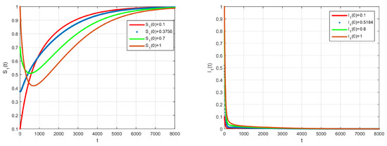
Figure 1.
Time series evolution depicting the dynamical behaviour of the system, using

Figure 2.
Time series evolution depicting the dynamical behaviour of the system (2), using
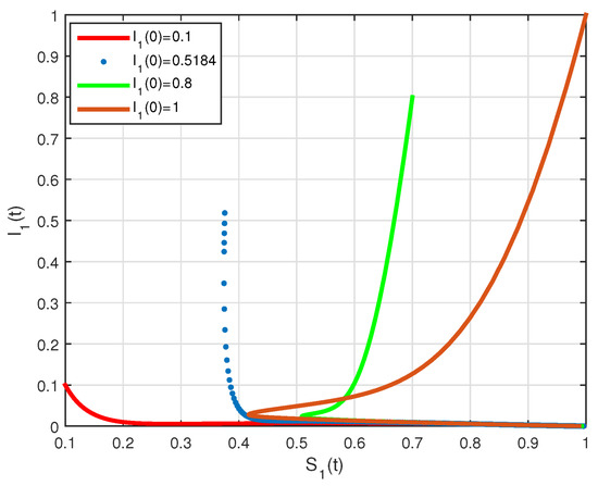
Figure 3.
State diagrams of vs. for system (2), using
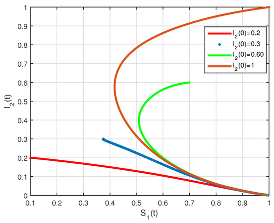
Figure 4.
State diagrams of vs. for system (2), using
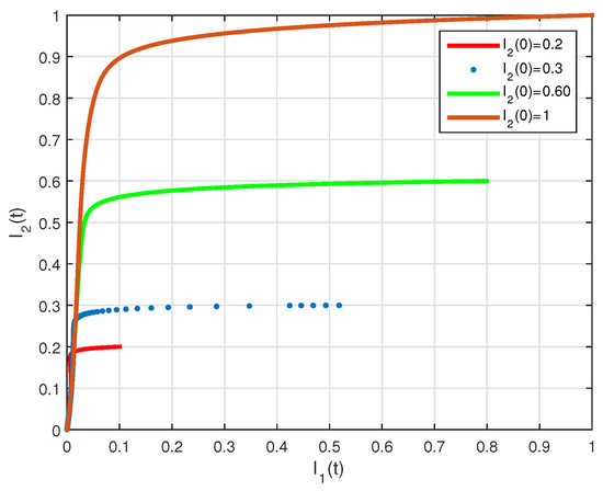
Figure 5.
State diagrams of vs. for system (2), using
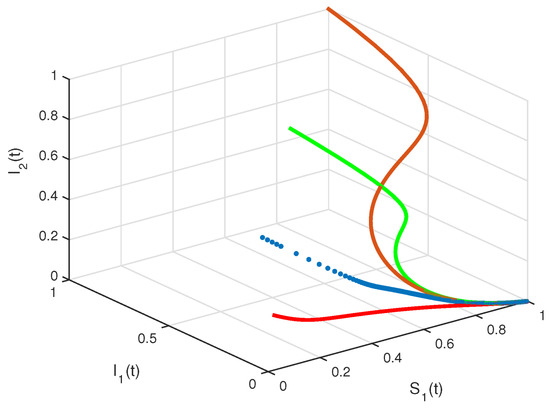
Figure 6.
State diagrams of system (2), using
Example 2.
Suppose that system (2) has the parameters
The basic reproduction number is such that and the system (2) has the endemic equilibrium of . The numerical simulation of system (2) with initial conditions is illustrated in Figure 7 and Figure 8, all these solutions converge to the . The phase diagram of with different initial conditions is given in Figure 9. Figure 10, Figure 11 and Figure 12, show the phase diagram of , and , with three initial conditions. The figures confirm the endemic equilibrium is globally asymptotically stable and all solutions converge to the endemic equilibrium point under the mentioned initial conditions.

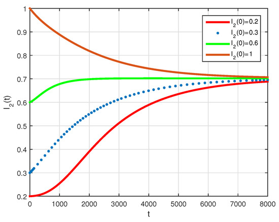
Figure 8.
Time series evolution of I2 for system (2), using
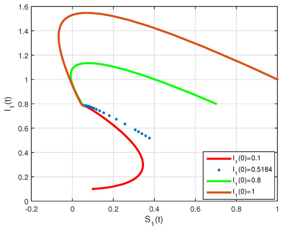
Figure 9.
State diagrams of vs. for system (2), using

Figure 10.
State diagrams of vs. for system (2), using
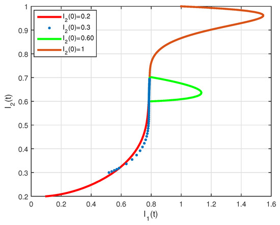
Figure 11.
State diagrams of vs. for system (2), using

Figure 12.
State diagrams of system (2), using
5. Conclusions
In the presented work, conditions for the global stability analysis of the Babesiosis disease system are established by the properties of Volterra–Lyapunov stable matrices and the classical method of Lyapunov stability. We used the modified method of Volterra–Lyapunov matrices as mentioned in Remark 1. The main advantage of this modification is that the higher dimensional matrices can be easily implemented. In each step, we reduce the dimensions of the matrix and use the property of the Volterra–Lyapunov matrices. This strategy simplifies the calculations and the proofs. The simulations confirm the results of the theories presented in this method.
Author Contributions
The authors declare that the study was realized in collaboration with equal responsibility. All authors have read and agreed to the published version of the manuscript.
Funding
Not applicable.
Institutional Review Board Statement
Not applicable.
Informed Consent Statement
Not applicable.
Data Availability Statement
Not applicable.
Acknowledgments
The authors express their sincere thanks to the anonymous referees for their rigorous comments and valuable suggestions helping to improve this paper.
Conflicts of Interest
The authors declare no conflict of interest.
References
- Sadiq, S.F.; Khan, M.A.; Islam, S.; Zaman, G.; Jung, I.H.; Khan, S.A. Optimal control of an epidemic model of leptospirosis with nonlinear saturated incidences. Annu. Res. Rev. Biol. 2014, 4, 560–576. [Google Scholar] [CrossRef]
- Panigoro, H.S.; Suryanto, A.; Kusumawinahyu, W.M.; Darti, I. Dynamics of an eco-epidemic predator-prey model involving fractional derivatives with power-law and Mittag-Leffler kernel. Symmetry 2021, 13, 785. [Google Scholar] [CrossRef]
- Ibrahim, O.M.; Ekundayo, D.D. COVID-19 pandemic in Nigeria: Misconception among individuals, impact on animals and the role of mathematical epidemiologists. Preprints 2020. [Google Scholar] [CrossRef]
- Hussain, T.; Ozair, M.; Okosun, K.O.; Ishfagh, M.; Awan, A.U.; Aslam, A. Dynamics of swine influenza model with optimal control. Adv. Differ. Equ. 2019, 2019, 508. [Google Scholar] [CrossRef]
- Rohith, G.; Devika, K.B. Dynamics and control of COVID-19 pandemic with nonlinear incidence rates. Nonlinear Dyn. 2020, 101, 2013–2026. [Google Scholar] [CrossRef]
- Momoh, A.A.; Abdullahi, H.M.; Abimbola, N.G.A.; Michael, A.I. Modeling, optimal control of intervention strategies and cost effectiveness analysis for buruli ulcer model. Alex. Eng. J. 2021, 60, 2245–2264. [Google Scholar] [CrossRef]
- Rezapour, S.; Mohammadi, H.; Jajarmi, A. A new mathematical model for zika virus transmission. Adv. Differ. Equ. 2020, 2020, 589. [Google Scholar] [CrossRef]
- Benz, K.; Rech, C.; Mercorelli, P.; Sergiyenko, O. Two cascaded and extended kalman filters combined with sliding mode control for sustainable management of marine fish stocks. J. Autom. Mob. Robot. Intell. Syst. 2020, 14, 28–35. [Google Scholar]
- World Organisation for Animal Health. Manual of Diagnostic Tests and Vaccines for Terrestrial Animals; OIE: Paris, France, 2020. [Google Scholar]
- Johnson, N.; Phipps, L.P.; McFadzean, H.; Brlow, A.M. An outbreak of bovine babesiosis in February, 2019, triggered by above average winter temperatures in southern England and co-infection with Babesia divergens and Anaplasma phagocytophilum. Parasites Vectors 2020, 13, 305. [Google Scholar] [CrossRef]
- Solorio-Rivera, J.L.; Rodrıguez-Vivas, R.I. Epidemiology of the babesiosis bovis. II. Epidemiologic indicators and elements for the design of strategies of control. BioMed 1997, 8, 95–105. [Google Scholar]
- Benavides, E. Considerations with Respect to the Epizootilogia of Anaplasmosis and Babesiosis in the Bovines; ACOVEZ: Bogotá, Colombia, 1985; Volume 9, pp. 4–11. [Google Scholar]
- Hartemink, N.A.; Randolph, S.E.; Davis, S.A.; Heesterbeek, J.A. The basic reproduction number for complex disease systems: Defining R0 for tick-borne pathogens. Am. Nat. 2008, 171, 743–754. [Google Scholar] [CrossRef] [PubMed] [Green Version]
- Aranda, D.F.; Trejos, D.Y.; Valverde, J.C.; Villanueva, R.J. A mathematical model for Babesiosis disease in bovine and tick populations. Math. Methods Appl. Sci. 2012, 35, 249–256. [Google Scholar] [CrossRef]
- Zafar, Z.U.A.; Rehan, K.; Mushtaq, M. Fractional-order scheme for bovine babesiosis disease and tick populations. Adv. Differ. Equ. 2017, 86. [Google Scholar] [CrossRef] [Green Version]
- Dang, Q.A.; Hoang, M.T.; Trejos, D.Y.; Valverde, J.C. Feedback control variables to restrain the Babesiosis disease. Math. Methods Appl. Sci. 2019, 42, 7517–7527. [Google Scholar] [CrossRef]
- Pourbashash, H. Global analysis of the babesiosis disease in bovine and tick populations model and numerical simulation with multistage modified sinc method. Iran. J. Sci. Technol. Trans. Sci. 2018, 42, 39–46. [Google Scholar] [CrossRef]
- Bentaleb, D.; Amine, S. Lyapunov function and global stability for a two-strain SEIR model with bilinear and nonmonotone incidence. Int. J. Biomath. 2019, 12, 1950021. [Google Scholar] [CrossRef]
- Upadhyay, R.K.; Pal, A.K.; Kumari, S.; Roy, P. Dynamics of an SEIR epidemic model with nonlinear incidence and treatment rates. Nonlinear Dyn. 2019, 96, 2351–2368. [Google Scholar] [CrossRef]
- Chen, X.; Cao, J.; Park, J.H.; Qiu, J. Stability analysis and estimation of domain of attraction for the endemic equilibrium of an SEIQ epidemic model. Nonlinear Dyn. 2017, 87, 975–985. [Google Scholar] [CrossRef]
- Liao, S.; Wang, J. Global stability analysis of epidemiological models based on Volterra-Lyapunov stable matrices. Chaos Solitons Fractals 2012, 45, 966–977. [Google Scholar] [CrossRef]
- Masoumnezhad, M.; Rajabi, M.; Chapnevis, A.; Dorofeev, A.; Shateyi, S.; Karga, N.S.; Nik, H.S. An approach for the global stability of mathematical model of an infectious disease. Symmetry 2020, 12, 1778. [Google Scholar] [CrossRef]
- Parsaei, M.R.; Javidan, R.; Kargar, N.S.; Nik, H.S. On the global stability of an epidemic model of computer viruses. Theory Biosci. 2017, 136, 169–178. [Google Scholar] [CrossRef] [PubMed]
- Zahedi, M.S.; Kargar, N.S. The Volterra-Lyapunov matrix theory for global stability analysis of a model of the HIV/AIDS. Int. J. Biomath. 2016, 10, 1750002. [Google Scholar] [CrossRef]
- Driessche, V.D.; Watmough, J. Reproduction numbers and sub-threshold endemic equilibria for compartmental models of disease transmission. Math. Biosci. 2002, 180, 29–48. [Google Scholar] [CrossRef]
- Cross, G.W. Three types of matrix stability. Linear Algebra Appl. 1978, 20, 253–263. [Google Scholar] [CrossRef] [Green Version]
- Rinaldi, F. Global stability results for epidemic models with latent period. IMA J. Math. Appl. Med. Biol. 1990, 7, 69–75. [Google Scholar] [CrossRef]
- Redheffer, R. Volterra multipliers I. SIAM J. Algebr. Discret. Methods 1985, 6, 592–611. [Google Scholar] [CrossRef]
- Redheffer, R. Volterra multipliers II. SIAM J. Algebr. Discret. Methods 1985, 6, 612–623. [Google Scholar] [CrossRef]
Publisher’s Note: MDPI stays neutral with regard to jurisdictional claims in published maps and institutional affiliations. |
© 2021 by the authors. Licensee MDPI, Basel, Switzerland. This article is an open access article distributed under the terms and conditions of the Creative Commons Attribution (CC BY) license (https://creativecommons.org/licenses/by/4.0/).