Abstract
We summarize our recent proposals for probing the -odd interaction at the LHC and its projected upgrades directly using associated on-shell Higgs boson and top quark or top quark pair production. We first recount how to construct a -odd observable based on top quark polarization in scattering with optimal linear sensitivity to . For the corresponding hadronic process we then present a method of extracting the phase-space dependent weight function that allows to retain close to optimal sensitivity to . For the case of top quark pair production in association with the Higgs boson, , with semileptonically decaying tops, we instead show how one can construct manifestly -odd observables that rely solely on measuring the momenta of the Higgs boson and the leptons and b-jets from the decaying tops without having to distinguish the charge of the b-jets. Finally, we introduce machine learning (ML) and non-ML techniques to study the phase-space optimization of such -odd observables. We emphasize a simple optimized linear combination that gives similar sensitivity as the studied fully fledged ML models. Using we review sensitivity projections to at HL-LHC, HE-LHC, and FCC-hh.
1. Introduction
The interaction between the heaviest particles of the Standard Model (SM), the top quark t and the Higgs boson h, is an important target for the LHC experiments. It is precisely predicted within the SM. The measured top quark mass and the electroweak condensate value v precisely determine the on-shell scalar (P- and -even) coupling , while P- and -odd interactions are absent. Beyond the SM, effective operators of dimension-6 can break this correlation and result in more general (pseudo)scalar couplings [1]
which reduce to the SM case at , .
-violating h couplings, like , are particularly interesting as any sign of violation in Higgs processes would constitute an indisputable New Physics (NP) signal. Existing data on Higgs production and decays is already precise enough to constrain any isolated modification of the top Yukawa to [2,3,4]. However, all existing measurements are based on -even observables with very limited sensitivity to -odd modifications of the top quark Yukawa. In principle, indirect collider bounds from Higgs decay and production (, ), and especially the low-energy bounds on electric dipole moments (EDMs) of atoms and nuclei that target specifically -odd effects [2,5,6], are currently more constraining than direct collider probes. However, these constraints are subject to assumptions about other Higgs interactions, and in particular in the case of EDMs also other contributions unrelated to the Higgs.
At the LHC it is possible to probe these couplings directly with two of the particles in Equation (1) on-shell (Since one cannot probe these couplings with all the three particles on-shell) in top-Higgs associated production processes and [2,3,4,6,7,8,9,10,11,12,13,14,15,16,17,18,19,20,21,22,23] (The loop induced partonic process depends on , , and already on the production side as it is dominated by the top quark loop [5]). The corresponding total cross sections scale as , ( also as ), and are thus poorly sensitive to small nonzero . Linear sensitivity to on the other hand can be achieved by measuring P- and -odd observables.
We have recently addressed this challenge by identifying observables with optimal sensitivity to a single -odd parameter in both and associated production at the LHC, which can be realistically measured and exhibit close to optimal sensitivity to -odd interactions between the Higgs boson and the top quark [24]. The proposed observables in are based on optimization of top-spin correlations previously studied in production [25]. Unfortunately, the overwhelming irreducible backgrounds make the channel impractical. On the other hand, in the case of this procedure becomes intractable in practice and our construction relies instead on - and P-symmetry arguments. In total, we can identify 21 different -odd observables that can be constructed out of 5 measurable final state momenta and an additional triple-product asymmetry [26]. Namely, assuming production with semileptonically decaying tops, we combine the final state lepton momenta , two b-jet momenta from decaying top quarks (although without discriminating their charges (Efficient b-jet charge discrimination could allow to construct further -odd observables, see e.g., [6,20])) and the Higgs momentum ph in different ways to construct C-even, P-odd laboratory frame observables wi [24].
Due to the high dimensionality and complexity of the phase-space in this process with top quarks decaying semileptonically, using the complete kinematical information accessible experimentally to construct an optimal -odd observable is challenging. To this end we have employed neural networks (NN) trained on Monte-Carlo generated samples to efficiently parametrize the weight function of events across the multi-dimensional phase-space in order to maximize the statistical sensitivity to [27]. We show how the required P- and -symmetry properties of the NN-based observables can be imposed a priori. Finally, we compare in terms of optimality, a general -odd NN function of the phase-space to a linear combination of manifestly -odd variables.
The present paper serves as a pedagogical review of the work first reported in Refs. [24,27].
2. Optimal CP-Odd Observable in the bW → th Process
2.1. Parton Level Analysis
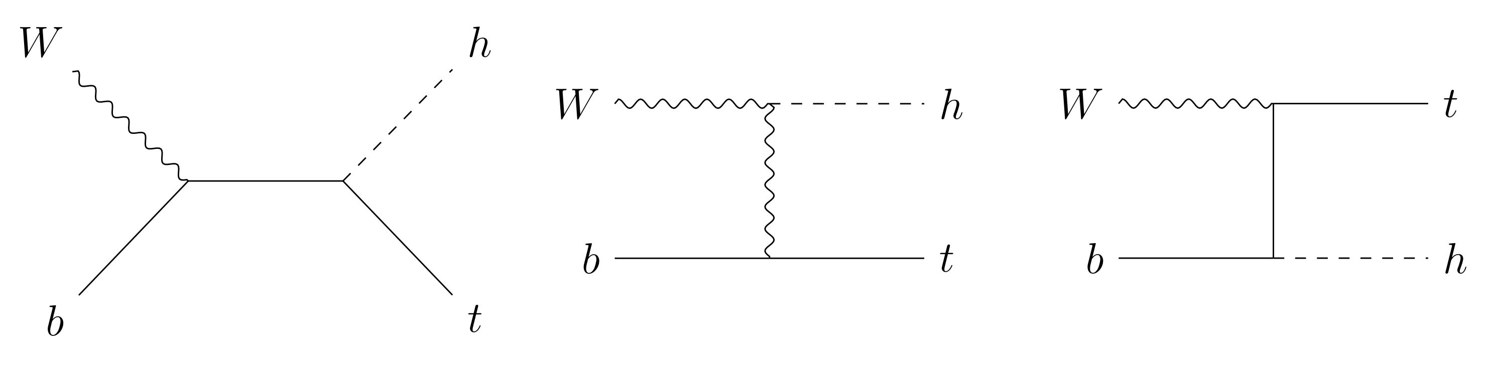
We begin by studying the effects of on top spin observables in the idealized case of single top quark production in partonic process . Here the complete polarized scattering amplitudes can be found in a compact analytic form. This process can actually be connected to a more realistic production in the high energy limit, where the W and b quark mass effects are negligible and the collinear emission of both initial state ‘partons’ can be described by the corresponding parton distribution functions. (See e.g., Section 3 of Ref. [28] for an extended discussion on the validity of this approximation) Three diagrams contribute to such parton level Higgs-top production in the SM, shown in Figure 1. Neglecting furthermore the mass (and thus the corresponding Yukawa coupling) of the bottom quark, we consider only the first two of the diagrams in Figure 1. The formalism presented here is based on Refs. [25,29,30]. First, we introduce the spin projection operator [31]
where is a top spin four-vector, defined in a general frame as
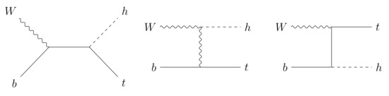
Figure 1.
Tree-level diagrams contributing to .
Vector is the top quark momentum and is an arbitrary unit vector that represents polarization of the top quark. The physical significance of is revealed if we make a rotation-free boost to the top rest frame where we find . Note that spatial component of four-vector in this case transforms as upon boost to the top rest frame. Therefore , , and corresponds to the polarization of the top quark in its rest frame. Projection onto a well defined polarization of the top quark is achieved by placing the projector (2) in front of the bispinors at the amplitude level:
Sum over top quark polarizations r then becomes
and the cross-section is linear in
Here the polarization vector is arbitrary while contains all the information about the polarization of the top quark in the given process. The parton level cross section can be written as
where is the initial state flux normalization and is the phase space volume. On the other hand, in the top rest frame it is convenient to introduce the spin density matrix as
such that the unpolarized cross section is proportional to . Here are the Pauli matrices. In the density matrix formalism, the expectation value of a generic operator is obtained as
In particular, the polarized cross section along is obtained as the expectation value of the projector:
One can determine the rest-frame coefficients from a, by comparing the expressions for polarized , expressed via Equations (7) and (11). The result of this matching are explicit expressions:
The rest-frame polarization of the top quark along a vector is given by the expectation value of ,
This observable can be determined for example by measuring the angular distribution of the charged lepton in the semi-leptonic top decay since the charged lepton in top decay is considered to be an almost perfect top spin analyzer, i.e., the angular decay distribution vanishes when the lepton momentum is opposite to the spin of t [32]. The angular distribution in the top rest frame
then allows for experimental extraction of the coefficients [32].
Here is an angle between the lepton and the polarization axis in the top rest frame. The above construction shows that the vector is an arbitrary unit vector defined in the laboratory frame. A particular choice implies that measures the top quark helicity. Another natural choice for is the W momentum , also known as the beam basis, which has to be carefully defined in actual collisions where the (symmetric) initial state does not allow to define forward and backward directions. Experimentally one has to reconstruct the top quark rest frame in order to be able to trace the angular distribution of the lepton with respect to the chosen and gain access to the coefficients . In the following we will show how to optimize the choice of such that the sensitivity to the -violating parameter is maximized.
In the center-of-mass frame we can define the W and t momenta as
where is the angle between the direction of the top quark and the W boson. We have set the azimuthal angle without loss of generality. The polarization vector components in this case depend on . Evaluation of the two diagrams in Figure 1 leads to the coefficients of the polarized cross-section. It turns out that in the coordinate system in Equation (15) the analytical expression for is linear in ,
whereas do not contain linear terms. Effectively this means that we should choose the vector to be orthogonal to the plane spanned by the W and t momenta in order to probe with linear sensitivity. Similar results have been reported in Ref. [18]. In pursuit of maximal sensitivity to we choose the polarization vector in each event as . In this case an interesting experimental quantity a two-fold differential cross-section
where we have approximated the intermediate top quark as a narrow resonance and is the differential production cross section for the top quarks polarized in the direction. Using Equation (11) and inserting we have , where is the initial flux normalization. Thus we can write Equation (17) as
Treating as a small perturbation we can integrate the distribution in Equation (18) with a phase-space dependent function f that would maximize statistical sensitivity of the integral to . It has been shown in Refs. [33,34] that such an optimal function should be the ratio of the -perturbation to the unperturbed distribution, in our case . The optimal observable is thus
where is the angle between and the lepton momentum in the top center-of mass-frame, as defined in the preceding paragraph. The index labels individual events. The prediction scales as ,
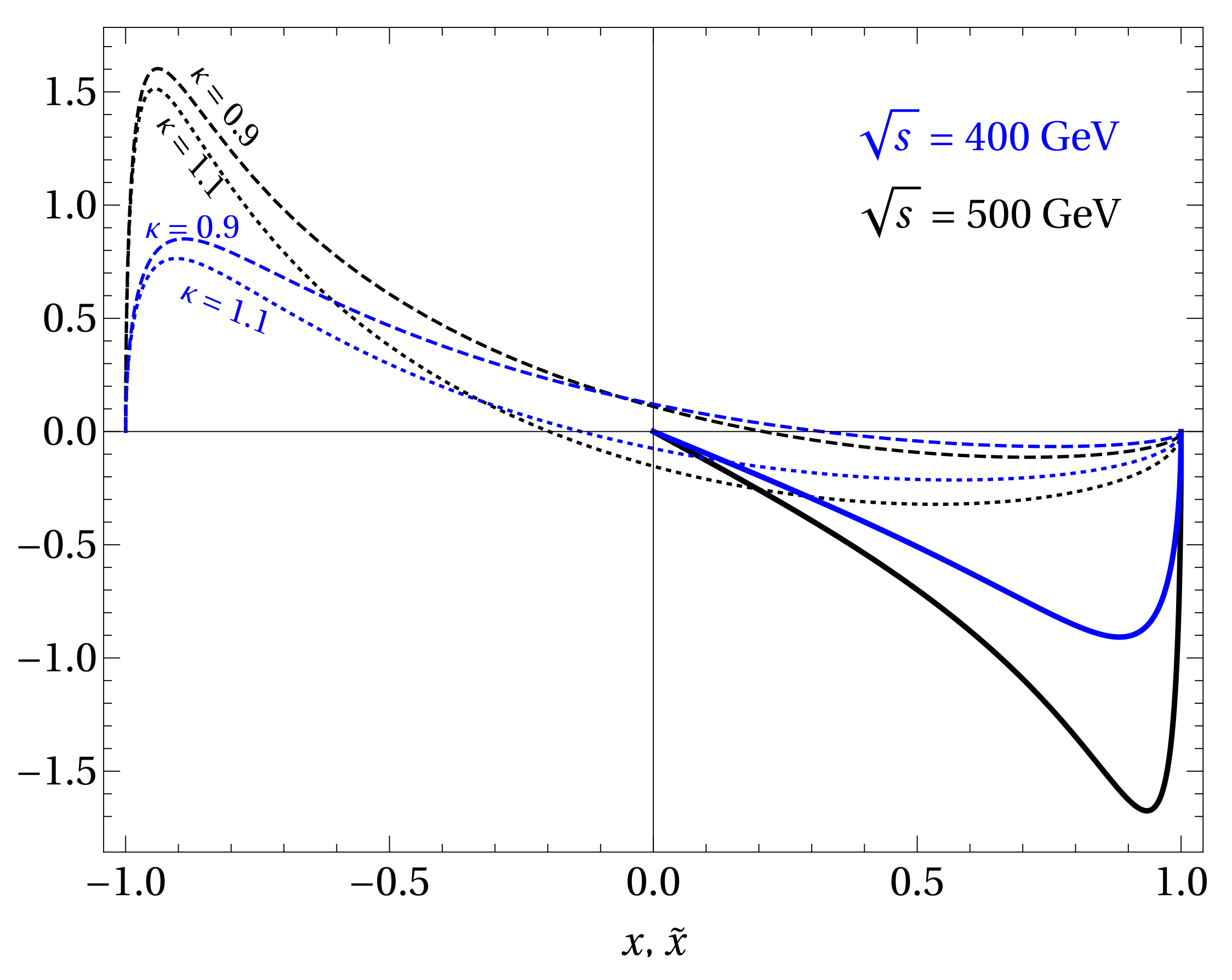
where we have integrated over and left the bounds for unspecified. The function is plotted in Figure 2.
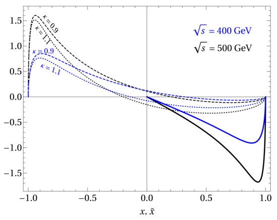
Figure 2.
Comparison of the (dashed and dotted) and (full line) polarization functions at representative CMS energies and two values of . We find that is independent of [24].
To carry over the presented formalism to the realistic case of collisions, we have to adapt the beam axis by referring only to experimentally accessible momenta. Using the reconstructed top momentum as a reference, we define the positive z-direction as the parallel top quark momentum projection . The top quark is then by definition in the positive hemisphere, , where is the angle between and . The optimal polarization direction with linear sensitivity now becomes upon which an experiment should measure the lepton angle . The cross-section distributions in and x are related via
where
The is flipped in the second term since for the polarization vector flips the direction compared to the previous definition, . The optimal observable in this case is finally
where the optimal weight function is again taken to be the ratio of the -perturbation to the unperturbed distribution (see Equation (21)), in line with Refs. [33,34]. In terms of experimental N data points with reconstructed and the observable is obtained as the following average:
In the limit where the observables are equal, . However in general the is expected to result in a weaker statistical significance due to our inability to determine the direction of the top quark with respect to the initial W. In Figure 2 we show that is large at negative x and we have , for representative values of the center-of-mass energy .
2.2. Hadronic Process
Here we demonstrate how to carry over the optimal -violating observable from parton level to the realistic case of collisions, but still neglecting reconstruction efficiencies and backgrounds. The parton level observable defined in Equation (23) can be adapted to this case with an additional integration over the parton distribution functions (PDFs). Since the hadronic cross section is a convolution of partonic cross sections it can be split into a -independent piece and the small perturbation proportional to , similar to the partonic cross section in Equation (21). Assuming that the Higgs decays into visible states, the missing is only due to the neutrino originating from the top decay. Thus we can reconstruct the top quark momentum and kinematic quantities of Equation (21). For hadronic collisions one can express the cross section as
and weigh the events with the optimal . To demonstrate the procedure we have used the Monte Carlo event generator [35,36] together with the Higgs Characterisation UFO model [37,38] (for an analysis of next-to-leading order QCD and next-to-next-to leading EW effects see Refs. [8,17,39], respectively) to incorporate the and couplings in the simulation of the signal. The procedure of extracting the optimal weight function from MC simulations and using it to produce the optimal observable goes as follows:
- Choose the bins for between and .
- Fix and extract from the MC simulation the mean in each of the bins. The obtained value corresponds to the weight in this bin, see Equation (25).
- Use this information to weigh experimental events bin-by-bin with . The normalization of is fixed by the requirement .
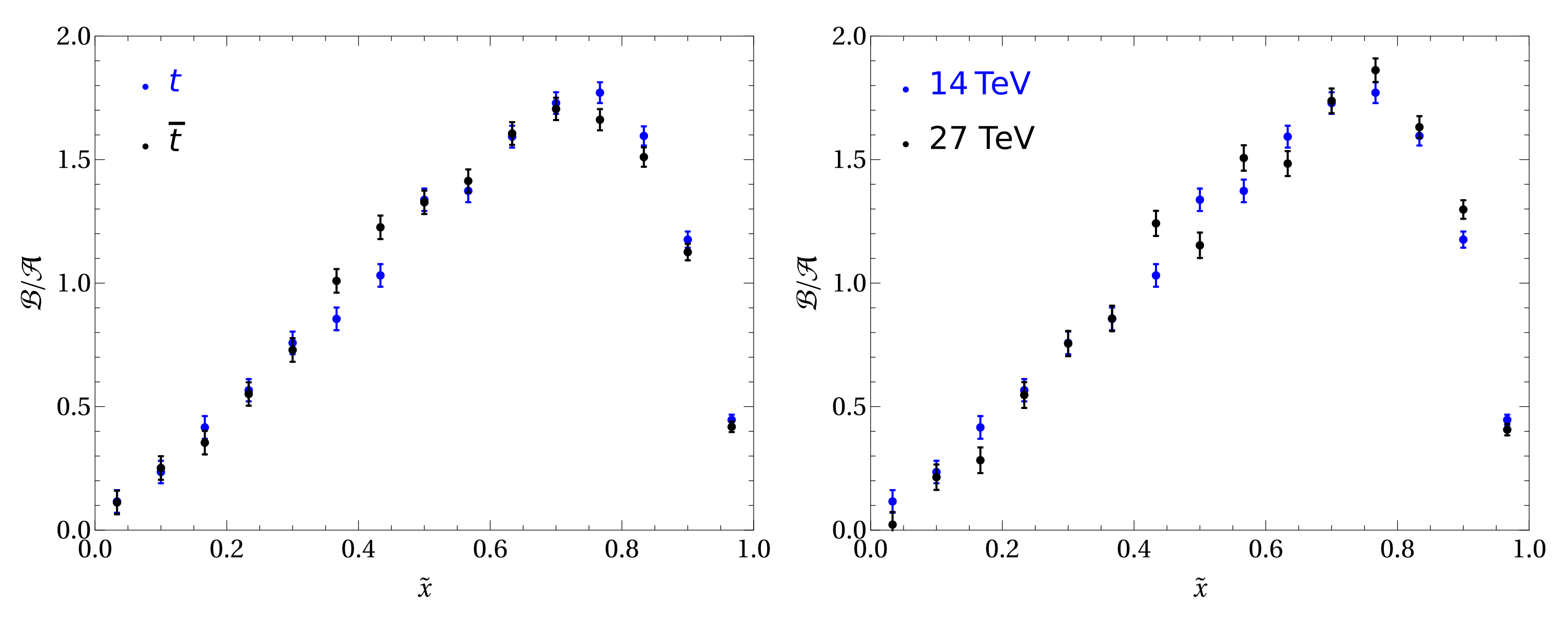
This optimization procedure is independent of the value as long as is sufficiently small. The resulting optimal weight is shown in Figure 3, where we compare it for different final states ( or ) and collision energies (14 or ). To assess the stability of the proposed method against higher order corrections we have extracted the weight function from simulations at NLO in QCD to estimate the systematic uncertainty associated with QCD effects and found that the difference is within 10% of the LO extraction. Finally, we can compare our optimized approach to the naïve extraction through the measurement of , which in turn corresponds to the case where the weight is independent of , i.e., . We define the signal significance of an observable as
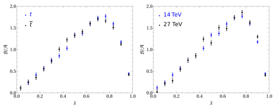
Figure 3.
Comparison of the optimal weight between the and processes extracted from MC simulations (left). The right panel shows the comparison between 14 and proton collision energies for . All plots are obtained using and with MC events [24].
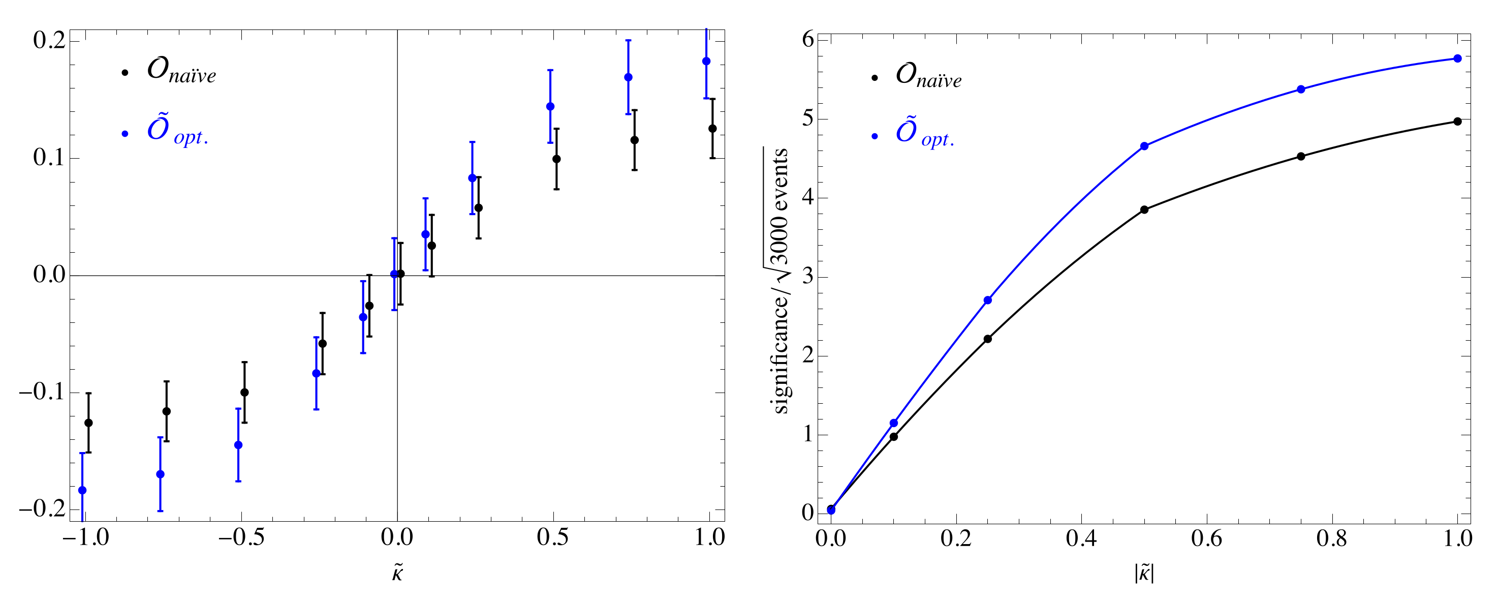
In Figure 4 we show the improvement of the significance when the optimal weight function is applied on simulated signal events without showering or reconstruction effects at 14 TeV.
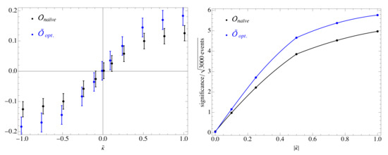
Figure 4.
Left: comparison of the optimized spin observable (blue dots) with the naïve observable (black dots) extracted from 3000 MC events at each choice of . Right: comparison of the significance (defined as the mean value divided by the standard deviation) per of the two observables, where N is the number of events [24].
2.3. Limits in the Plane from at Event Reconstruction Level
In order to make closer contact with experiments, we can also include the effects of parton showering, detector response and background processes. In our analysis we have used to generate events at leading order (LO) in QCD for the signal process plus the conjugate process with at 14 TeV High-Luminosity LHC (HL-LHC) and 27 TeV High-Energy LHC (HE-LHC) center-of-mass energies. (Note that our procedure of obtaining an optimal observable does not depend on the h decay products, therefore this analysis should be taken as a proof of concept with potential for future improvements using e.g., multiple h decay channels) Event generation was performed for multiple values of (, . The parton level events were subsequently showered and hadronized with [40], and jets are clustered with the anti- algorithm using [41]. For detector simulation and final state object reconstruction (e.g., lepton isolation and b-tagging) we used [42] with the default ATLAS parameters in . The dominant background process in this analysis is production with additional associated jets. We included this background by generating samples, with one of the tops decayed into the semi-leptonic channel and the other one decayed into the hadronic channel, produced in association with 0, 1, and 2 hard jets. In order to correctly model the hard jets’ distributions, we merged the matrix element computations with the MC shower using the [43] prescription. For the event selection we demand the following basic requirements:
- Exactly 3 b-tagged jets with and GeV,
- One additional (non-tagged) light jet exclusively in the forward direction with and GeV,
- One isolated light lepton with and GeV.
In addition, we further select events with one reconstructed Higgs and one reconstructed top quark as follows: first, we calculate the three possible invariant masses from the three reconstructed b-jets () and only keep the event if at least one pair satisfies GeV. For such events, we select as the Higgs decay candidate for the pair of b-jets with the invariant mass closest to the Higgs mass. The remaining non-Higgs b-jet is then assumed to come from the top-quark decay. Next, we reconstruct the top-quark by requiring that the combined invariant mass of the remaining b-jet, the lepton, and the neutrino (also reconstructed by assuming it to be the unique source of missing energy in the event) to fall inside the mass window of the top-quark defined by GeV. In order to further reject the backgrounds, events with a reconstructed Higgs and top are selected if the combined invariant mass of the b-jets originating from the Higgs and the light jet satisfies the cut GeV [44]. The final selection efficiency for the signal in the SM is (), while for the background it is () at 14 TeV (27 TeV).
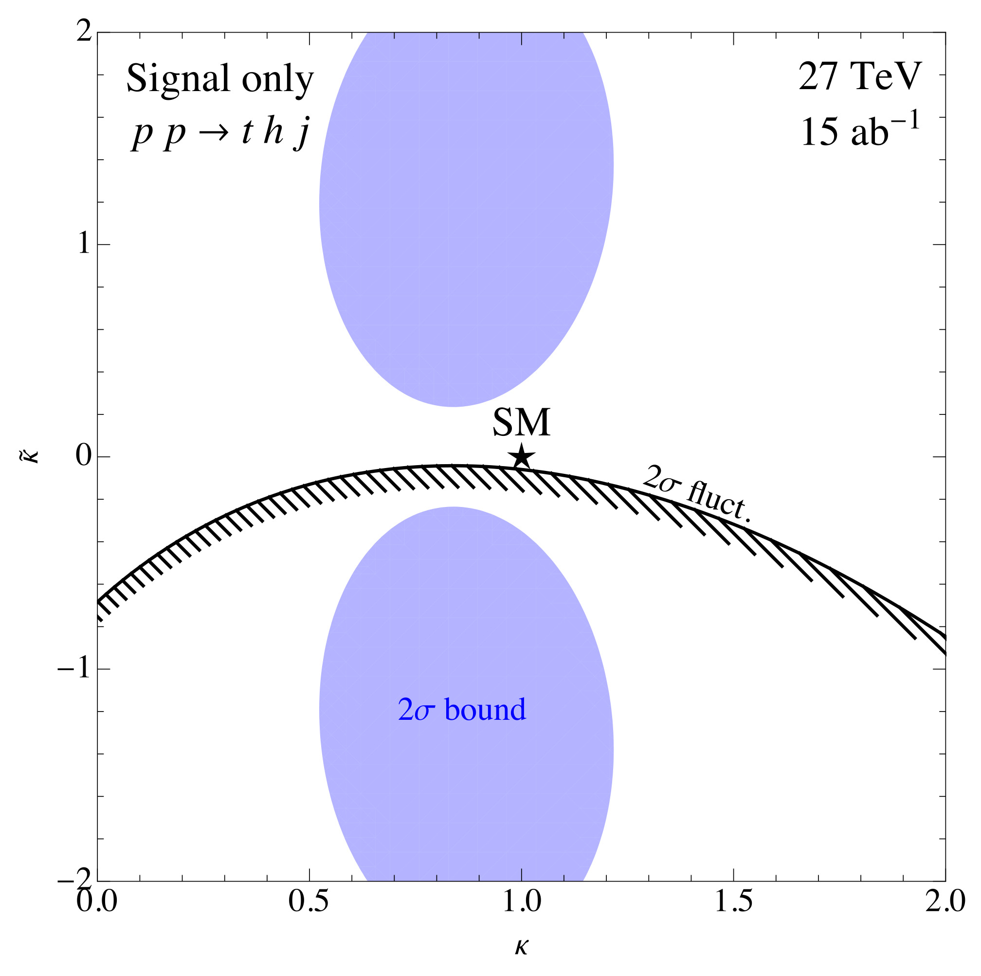
As we fully reconstruct the system and have access to the lepton momentum from the top decay we have all the necessary information for measuring the optimized spin observable. We use the optimal weight function (Figure 3) extracted from the MC simulations to construct a with an appropriately weighted signal process. Our results for generated in the SM are given by the exclusion limits (shaded blue) shown in Figure 5 for the HE-LHC at a luminosity of . As can be seen in Equation (23) the observable is normalized to the cross section, which contains terms , , as well as a linear term in and a constant term due to second diagram in Figure 1, whereas the numerator is proportional to . The behaviour of close to the SM point is thus linear in , whereas the cross section has a minimum in close to . In the large coupling regime converges to a small value which depends on the direction in which we make the limit . The exclusion has an elliptic shape as shown by the blue contour in Figure 5. We also present the limit (given by the black elliptic contour) assuming a positive excess above the SM expectation corresponding to a measurement of the optimized spin observable of whose size and error are statistics-driven. Because of the nature of our observable, the signed fluctuation gives rise to asymmetric limits in the direction. In the direction the bounds are also not symmetric as production contains linear terms. Finally, in order to include background effects, the same statistical analysis would have to be repeated including the background in the fit. However, even with a large background rejection as implemented above, the irreducible background is simply too large and the signal is completely diluted leading to a signal significance of only at 14 TeV (27 TeV) at a luminosity of (). This effectively precludes any meaningful extraction of bounds on from a fit to . We leave the possibility of further optimizing the cuts in order to reduce the backgrounds or including other Higgs decay channels as a future challenge. In the remainder of this review we instead focus on the related but more abundant process of associated top quark pair and Higgs boson production.

Figure 5.
Bounds in the plane using the optimized observable for the single-top associated production with a Higgs boson. The blue shaded region corresponds to the () exclusion zone assuming the measurement of the SM at the HE-LHC (15 ab). The black line and stripes shows the excluded region for a positive fluctuation at the HE-LHC (see text for details) [24].
3. CP-Odd Observables in the Process
In this Section we introduce laboratory-frame accessible and phase-space optimized -odd observables in the process in which both top quarks decays semi-leptonically: and . This process has a higher S/B ratio compared to and has indeed been measured by the LHC collaborations [45,46] (For the state of the art predictions of the differential distributions see e.g., Ref. [39]) The top quarks in are known to be unpolarized, independent of the value of [2]. The information on the underlying and parameters is in principle contained in the correlations among the top quark spins, however due to the experimental difficulties of extracting the top quark polarizations in this process, this approach is unfeasible. This is the reason we focus in this Section on manifestly -odd observables, directly sensitive to and easily accessible by measurements of final-state momenta in the lab frame.
3.1. Laboratory Frame -Odd Observables in Production
The accessible final-state momenta [6] of this decay in the lab frame are 3-momenta of b-jet , -jet , 3-momenta of leptons and , and 3-momenta of the Higgs . In practice differentiating between b-jet and b-jet is difficult (For recent attempts in extracting the charge of theb-jet see References [47,48,49,50]), therefore we should consider only observables which are invariant under pb ↔ pb transformation. We construct these observables from 3-vector quantities with well defined C and P eigenvalues, that are given in Table 1.

Table 1.
Vector quantities with well-defined C and P eigenvalues in 3 dimensional Euclidean space. More complicated objects with well-defined C and P eigenvalues can be constructed using variables in this table.
We use quantities in Table 1 to construct -odd variables of mass-dimension 5, that are C-even and invariant under transformation. In order to systematically obtain all distinct ’s we proceed as follows. First, we construct variables of the form (Notice that the possibility of a nested cross product can also be reduced to this form) using for . Doing so, we find 150 potential quintuple products. We symmetrize them with respect to C-conjugation and transformation. The non-zero quintuple products are variables, however they may be linearly dependent. Indeed some of the obtained ’s are connected via the following Euclidean identity
which can be written as:
where , , and are four arbitrary vectors in 3 dimensional Euclidean space. The sign of individual terms in the last expression corresponds to the sign of the cyclic permutation of the four vectors.
The first class of ’s involves and in the mixed product, in the scalar product. Both products are invariant under :
The second class involves and/or in both mixed and scalar products:
The third class involves mixed product of , and :
There are further possibilities with a mixed product multiplied by one of 8 C-even, even scalar products . Since the mixed product itself already has the desired symmetry properties, those 8 quintuple products do not bring additional new information, with respect to a mixed (triple) product that is our final observable:
Note that there are nonlinear relations between ’s, such as , that we do not exploit to further reduce the set. Namely, ratios of ’s can contain singularities in the available phase-space and as such would be difficult to reconstruct by a neural network optimizer.
All the ’s are normalized by the lengths of the vectors that enter as factors in the scalar products,
and the upper bound is generally valid. For cases when has a vector present both in the mixed and scalar products, e.g., , and furthermore with , a stricter upper bound applies (for ).
Having constructed manifestly -odd variables , we now show how they can be used to extract information on in an optimal way. The production cross section can be written as
where are -even phase space variables, A is a manifestly -even and B is a manifestly -odd function of : . The dependence is due to the interference of scalar and pseudoscalar amplitudes. A simple -odd observable is an average of a single variable
where N is the number of experimental events. The standard deviation of such an observable is given by
For large enough N the distribution of is approximately Gaussian and the corresponding significance of this observable is:
Equation (55) holds for and their linear combinations. By studying the behavior of all 22 such observables on MC simulations of with semi-leptonically decaying top quarks we have found that and are the most promising in terms of their significance. Our next aim is to show how one can achieve better sensitivity to by introducing optimized observables in two directions: the phase-space optimization of a single and a construction of an optimal -odd observable as a combination of all available s.
3.2. NN-Based Optimized -Odd Observables
Due to the high dimensionality and complexity of the phase-space in the process with top quarks decaying semileptonically, we rely on neural networks (NN) trained on Monte-Carlo generated samples to efficiently parametrize the weight function of events across the multi-dimensional phase-space in order to maximize the statistical sensitivity to . We note that existing general purpose ML inference tools are already able to optimize sensitivity to a given parameter (see e.g., Ref. [51]). The purpose of our work was to do so in an economic way that manifestly respects the symmetries of the problem.
We implemented the training and evaluation of neural networks using the framework [52]. In all cases, we used a sample of events generated at LO using [35] together with the Higgs Characterisation UFO model [37,38] with . We split the sample into separate training (7.5 M) and test (2.5 M) samples. After training at fixed we also tested the observables at other values of and , both ranging from to 1. In these tests 1 M events have been used.Unless stated otherwise the results are shown for events in collisions at 14 TeV. We randomly initialized the neural network weights using the default Glorot uniform initializer and used the Adam optimizer with a custom varying learning rate where e is the current epoch and the initial learning rate is set to . We use for the activation function. We trained all networks using the novel loss function
where the and the standard deviation are to be calculated over all events in the sample. The loss corresponds to the inverse of the significance-squared of the observable that should be minimized in order to achieve optimal statistical sensitivity. Here N is the size of the event sample, are the free neural network weights and biases and stands for the values of -even and/or -odd phase-space variables in the given event. We emphasize that such a choice of the loss function is unique to the problem at hand - we are using the optimization procedure to directly maximize the significance of each considered observable. We can avoid over-fitting of the training sample by stopping the training when at least 30 epochs have passed and one of the following two criteria is satisfied: either the running average of 20 training losses saturates to or the running average of 20 test losses increases for 5 epochs in a row. We keep a model history and in the end choose the best model in terms of test loss. In practice we found that mostly the first condition terminates the training loop, and the best model is usually the model from the final epoch of training. In order to determine the optimal NN architecture we performed a scan over a set of possible NN configurations with up to 2 hidden layers and up to 9 nodes per NN layer. (We have also considered an automated algorithm to determine the optimal NN architecture (i.e., Hyperopt [53], see also Ref. [54] for one of its recent uses.). Here instead we present results of manual scans over a set of possible NN configurations in order to have better control over the NN parameters. We found the results of both approaches comparable. We choose this cutoff for representational purposes, however we have checked that our results do not change significantly when using larger networks, namely up to three hidden layers of 30 nodes each.)
3.2.1. Phase-Space Optimization of a Single
First we present the optimization of the and variables based on phase-space averaging. We do not follow the optimization procedure based on separating A and B in Equation (52) since this would require cumbersome multidimensional binning [33]. We use a vector of easily accessible -even Mandelstam variables :
Our goal is to find the optimal -even weight function , which should be used to calculate the weighted average of . The function f takes -even quantities as inputs, therefore we expect its dependence on to be of the form
Using (52) we can now express the observable
with the usual definition of the average (The phase space average of a function is defined as ). The integration region in space is symmetric with respect to the transformation , therefore integrals of the arguments which are anti-symmetric in vanish. Due to this reason all contributions to the expected value of the observable are proportional to odd powers of . The large dimensionality of the phase-space suggests the parameterisation of the function by means of an appropriate NN. In terms of the loss function (56) we have .
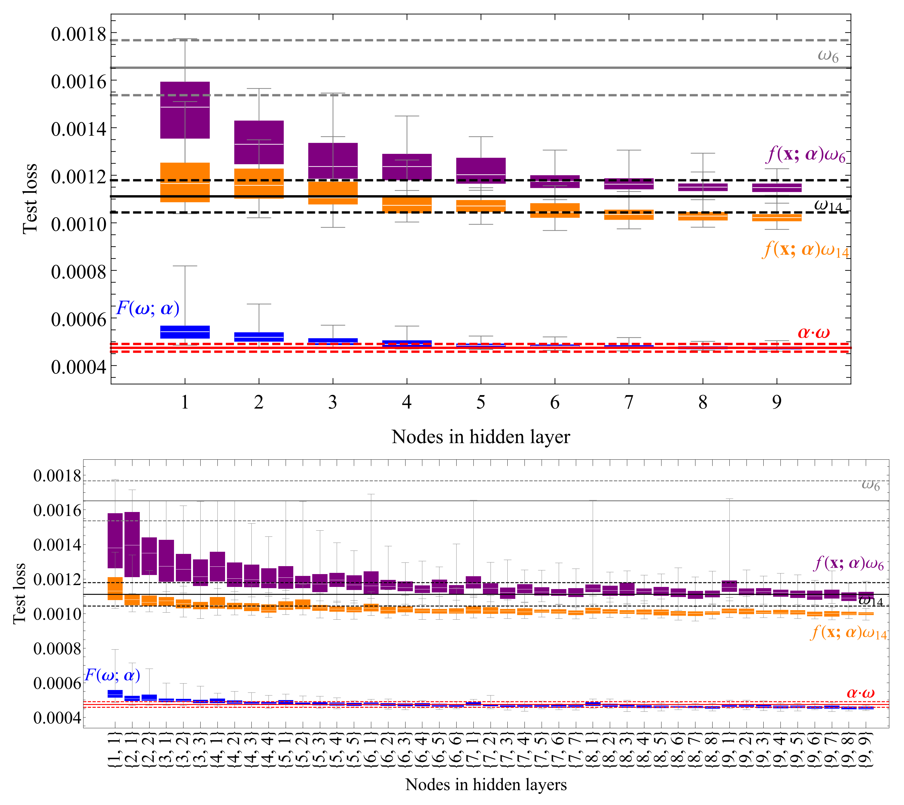
To understand the impact of using different possible neural network architectures, we have performed a manual scan over a set of neural network configurations. The input layer has 5 nodes (one per each component) and the output layer has one node resulting in a scalar . We studied networks with a single hidden layer of 1–9 nodes and double hidden layer networks with 1–9 nodes each, constraining the number of nodes on the second hidden layer to be smaller than or at most equal to the number of nodes on the first hidden layer. The results of the converged test losses of 50 different random weight initializations per configuration are shown on Figure 6 in the purple box plot for the case of and the orange box plot for the case of . The plain -based observable is shown in gray, with the dashed lines denoting its statistical uncertainty, while the same holds true for plain in black. We found that the phase-space optimization of gives a noticeable improvement over plain when using a large enough network. Interestingly, seems to be close to optimal on its own, as the phase space optimization does not introduce noticeable improvement. Moreover, the optimized gives a similar performance to , hinting that we have reached maximal performance achievable with a single .
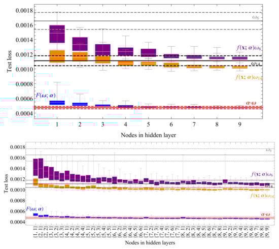
Figure 6.
A scan in terms of the test loss (sample size 2.5M, ) over neural network configurations with one (upper plot) or two (lower plot) hidden layers for the phase-space optimized and (59) shown in the purple and orange box plot and the generalized (Section 3.2.2) shown in the blue box plot. The spread in all cases corresponds to 50 different random weight initializations per configuration. For comparison the plain and are shown in gray and black with the dashed lines showing their statistical uncertainty. The first order approximation of , defined in Equation (60), is shown in red as described in Section 3.2.3 [27].
To test how well the resulting networks generalize to other values of we used the 50 converged models to calculate the dependence of the resulting observable significances with respect to on the aforementioned fresh sets of 1 M events per . This is shown on Figure 7 where a consistent improvement over simple can be seen at all considered , while again a marginal improvement is confirmed for , with the optimized hovering around .
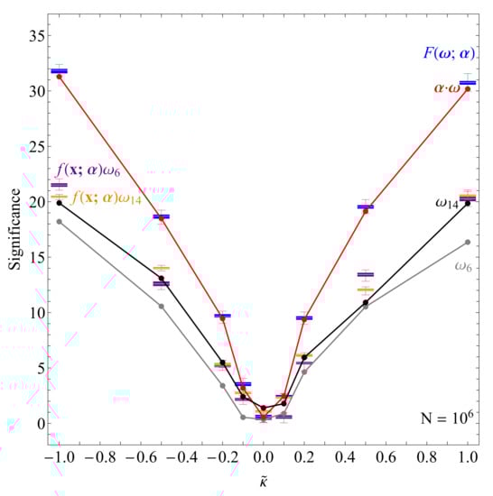
Figure 7.
Comparison of the significances (defined as the mean value divided by the standard deviation) of all the observables considered in this work with respect to and at fixed . The results correspond to 1M events per at 14 TeV. Plain in gray, in black, phase-space optimized and (59) in purple and orange, anti-symmetrized neural network (Section 3.2.2) in blue and the first order approximation of the latter in red (Section 3.2.3). See text for details on each observable [27].
As the results of optimizing single and point to a maximal performance possible using a single and the chosen set of phase space variables, we now turn to the rest of the ’s. In the next subsection we consider a more general case where the -odd observable itself is parameterized with a neural network.
3.2.2. Neural Network as a -Odd Observable
We consider the case where the output of the neural network is a -odd quantity that defines our observable. To this end, we build a network with 22 inputs, one per each , and one output , which is correctly anti-symmetrized so that . In terms of the loss function (56) we have . Note that since we include the complete irreducible set in this non-linear construction, it effectively also covers the case of a simple phase-space optimization of any (linear combination of) , since all relevant -even phase-space variables can be recovered by taking suitable products of .
We again carried out the study of the dependence of the network size with respect to the test sample loss, including non-negligible uncertainties associated with random weight initializations. We scanned the neural network architecture parameter space in the same way as in the previous case, starting with a single hidden layer of 1–9 nodes, then adding an additional hidden layer with the number of nodes smaller than or equal to the number of nodes on the first hidden layer. For each configuration we ran 50 trainings with different random weight initializations. The results are shown in Figure 6 in the blue box plot. We find a considerable improvement over the phase-space optimizations of or . The improvement is consistent in the entire range of and is most striking at large .
Again we can check the generalizing power of the resulting observables to other by fixing the model configuration to and calculating the significance of the resulting observables with respect to . The results are shown on Figure 7. We find a consistent improvement over the previous case across all considered . A noticeable improvement in the significance can be seen. In order to better understand the physics underlying the optimization, we next consider this model in the leading order approximation in .
3.2.3. First Order Approximation of ;)
To address the arbitrariness of the neural network architecture choice and to better understand the underlying physics, we finally consider the first order approximation of the function , which can be expanded in a Taylor series for , since for most events the values of the -odd variables are small: , . In the first order approximation the optimal -odd observable can be written as
where are parameters that satisfy a subsidiary condition . Their values can be found by maximizing the significance:
The left side of the expression above can be expanded in the following way:
where in the last step we take outside the , for example . By assuming we have . From this, together with the condition in Equation (61), it follows that the expression in the curly brackets of Equation (62) must be equal to 0. Hence, we obtain a system of 22 quadratic equations (The problem is equivalent to a single neuron NN with 22 inputs and one output without the activation function and the bias term)
where and the matrices are given by (Notice that by definition for all i and k, therefore for all k)
The system of equations in Equation (63) can be solved numerically. The solution vector is undetermined up to a real non-zero constant. We normalize it such that and choose the solution with mostly positive values.
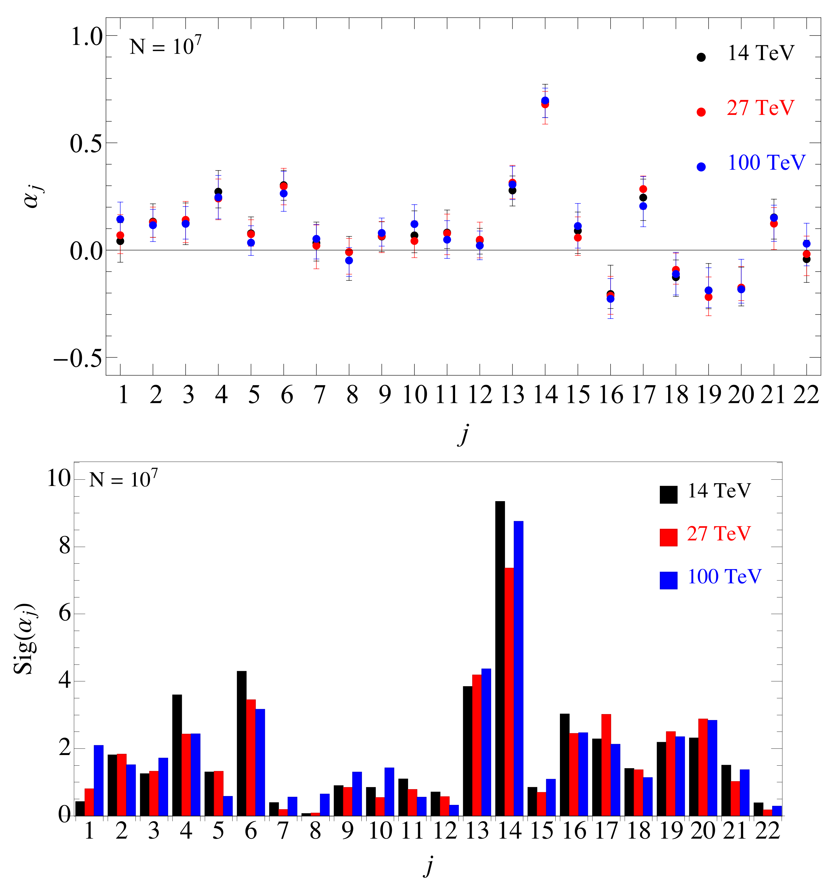
We used this approach to extract the optimal weights from events generated with at 14, 27, and 100 TeV. We also estimated the uncertainty associated with the optimal weights using the following procedure: First we estimate the statistical spread of the significance obtained with optimal . Next we allow a single to float in the intervals , where is chosen such that the decrease of the significance due to the change in corresponds to the statistical spread of the significance. We perform an efficient scan around the optimal vector in its 22-dimensional neighborhood using spherical coordinates to trivially fulfill the normalization constraint . We approximate the significance with a quadratic function around the extremum to find independent, uncorrelated directions in the -space. With this procedure we determine how sharply the optimal are defined. In practice, we estimated the statistical error of the significance using events. Clearly the uncertainties are larger for smaller chosen sample size. The results of this approach are shown in Figure 8, where the upper (lower) panel shows the estimated error (significance) for each at 14, 27, and 100 TeV. A comparison of the observable to other approaches discussed previously is shown in Figure 7. We reach a similar level of improvement compared to the full network with significantly fewer parameters.
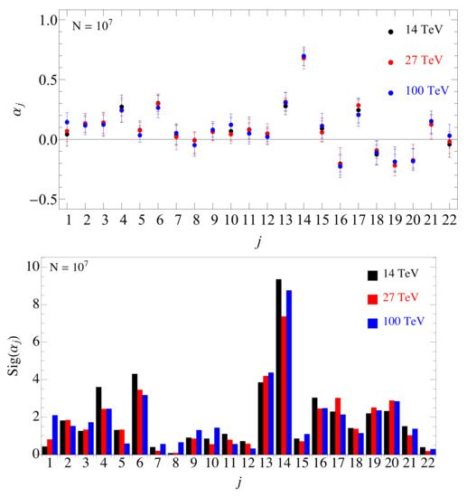
Figure 8.
Optimal weights of the linear observable defined in Equation (60). The upper plot shows uncertainties of , estimated using the expected statistical errors of the observable significances, see text for details. The lower plot shows the significances of (defined as their central value divided by their estimated uncertainty) [27].
3.3. Bounds in the Plane
We could now produce the bounds in the plane by varying both and at generator level and including showering and hadronization effects using and detector effects using with the default ATLAS simulation card. As the is followed by semileptonic top decays and decay, our signal is defined as 4 b-jets and two oppositely charged leptons ℓ. We included the main irreducible background with both tops decaying semileptonically and used the event selection requirements:
- jets of any flavor with and GeV.
- of the above jets are b-tagged.
- 2 oppositely charged light leptons with and GeV.
Furthermore, in order to identify the b-jets from t, decays we counted the number of tagged b-jets and performed the following selections: if , we compute the invariant masses of all possible b-jet pairs and select the pair with invariant mass closest to the Higgs mass GeV. If the selected pair falls inside the Higgs mass window ( GeV) we removed the pair from the list of b-jets and selected from this list the highest b-jets as our candidate top quark decay b-jets. However, if we computed all possible invariant masses where j are non-b jets in the event. We selected as the candidate the pair that minimizes and falls inside the Higgs mass window GeV. The remaining two b-jets are taken as the candidate top quark decay b-jets.
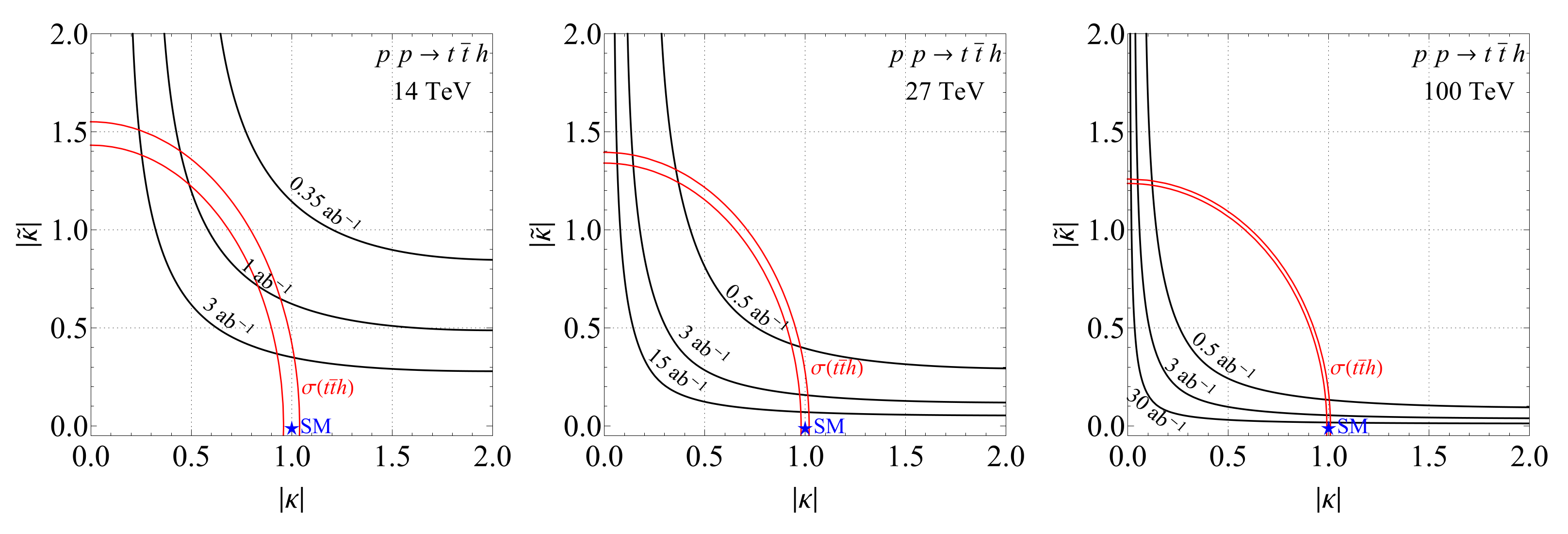
We present the bounds for HL- and HE-LHC, FCC-hh by using the optimal observable (60) with the weights shown in the upper plot of Figure 8. The bounds coming from a null result up to the expected statistical uncertainty for different luminosities at different energies are shown on Figure 9, where we also show the expected sensitivity to from the production cross-section measurements using the projected uncertainties of at HL-LHC, HE-LHC [55] and FCC-hh [56], respectively. For direct comparison with [24] we also show the expected bounds from using a single and have checked that using does not change the single bounds significantly.
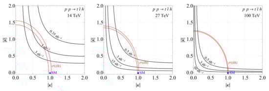
Figure 9.
The exclusion zones in the plane using the optimized observable by assuming a null result at HL-LHC, HE-LHC and FCC-hh for different luminosities (left: 14 TeV; middel: 27 TeV; right: 100 TeV). The projected sensitivity of production cross-section measurements is shown in red, see text for details. At 14 TeV exclusion of can be achieved using with which corresponds to the final integrated luminosity of the LHC [27].
A consistent improvement of sensitivity compared to using single can be achieved by using the optimized combination of ’s, constraining the parameter space significantly in orthogonal directions compared to the cross-section measurements. Interestingly the significance improvement is consistent between partonic events and after including shower, detector effects, as well as the dominant background and realistic object reconstruction, even though the optimization was performed at parton level only. This robustness is a welcome benefit of the method, since the computationally costly optimization procedure does not appear to be sensitive to modeling of the hadronic final states and detector effects. It is also reassuring that the optimization does not significantly rely on specific phase-space regions particularly affected by the background. We expect the results to be also robust against higher order QCD corrections as in the case of , where we have checked this explicitly.
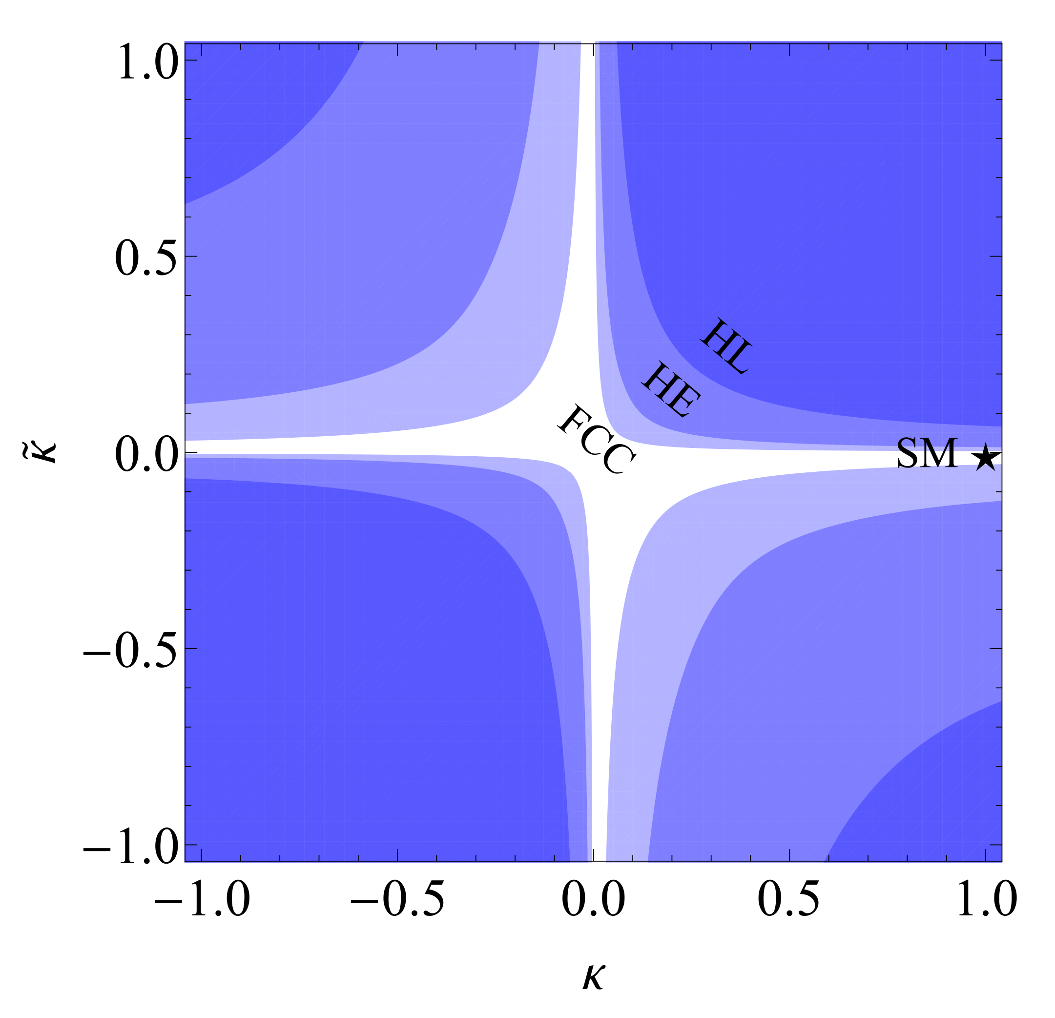
We show the sensitivity of the optimized observable to the sign of (and ) in Figure 10 by assuming the measurement of a positive statistical fluctuation of the SM case, which in our estimate corresponds to the measurement of , and for HL-LHC (3 ab), HE-LHC (15 ab) and FCC-hh (30 ab) respectively.
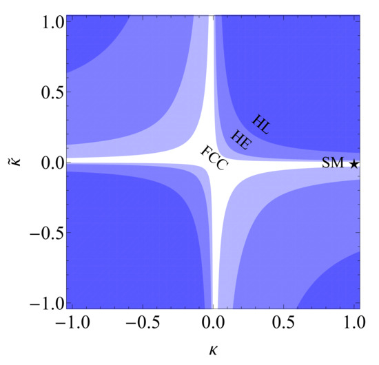
Figure 10.
The exclusion regions at HL-LHC (3 ab), HE-LHC (15 ab) and FCC-hh (30 ab) by assuming a measurement of a positive fluctuation in the optimal observable (60) [27].
4. Conclusions
In order to establish, directly and with minimal additional assumptions, the presence of a -odd component of the top quark Yukawa (), we have studied manifestly -odd observables in and production at the LHC and its prospective upgrades.
For the final states we have relied on the possibility of reconstructing the t quark momentum and accessing the t polarization. We have identified a particular polarization direction which is perpendicular to the plane, where the top polarization along this direction would undoubtedly point to the presence of the -odd coupling . We have presented a method for optimizing the phase space dependent weight and shown its sensitivity at the HL- and HE-LHC for the semileptonic top and mode. The handful of signal events offer discriminating power, sensitive to the sign of , however the irreducible background due to +jets severely dilutes the sensitivity of the proposed observable.
On the other hand, production has a considerably larger cross section at LHC energies compared to , while suffering more moderately from irreducible backgrounds. Due to the complexity of the final state kinematics with multiple undetected particles we have in this case proposed variables that only depend on the lab-frame accessible momenta and are manifestly P- and -odd. Furthermore, we have studied the prospect of their phase-space optimization, parameterizing the optimal weight functions with neural networks. In particular, we have studied a general -odd observable, parameterized directly by a anti-symmetric neural network, which results in better performance compared to any individual . Finally, we have studied the first order approximation of this network as a linear combination of the -odd observables, producing a simpler and more robust observable, . One benefit of using optimized at parton level is that it retains close to optimal sensitivity to the -odd coupling even after detector simulation, event selection and reconstruction, allowing to probe directly at HL-LHC, HE-LHC and FCC-hh. We have found that, at the end of Run 3, the LHC will exclude with confidence, while FCC-hh will be sensitive to . Note that these observables represent highly complementary probes of the top Yukawa sector compared to cross-section measurements. In particular in their optimized form they would allow to break the degeneracy in the plane and significantly reduce the allowed parameter space even at modest sensitivities accessible at the (HL)LHC.
Author Contributions
Conceptualization, J.F.K. and N.K.; methodology, D.A.F. and A.S.; software, B.B. and A.S.; validation, D.A.F., J.F.K. and N.K.; formal analysis, N.K. and A.S.; data curation, A.S.; writing—original draft preparation, B.B.; writing—review and editing, J.F.K., N.K. and A.S.; visualization, A.S.; supervision, J.F.K. and N.K.; funding acquisition, J.F.K. and N.K. All authors have read and agreed to the published version of the manuscript.
Funding
The authors acknowledge the financial support from the Slovenian Research Agency (research core funding No. P1-0035). This article is based upon work from COST Action CA16201 PARTICLEFACE supported by COST (European Cooperation in Science and Technology).
Institutional Review Board Statement
Not applicable.
Informed Consent Statement
Not applicable.
Data Availability Statement
Not applicable.
Conflicts of Interest
The authors declare no conflict of interest.
References
- Aguilar-Saavedra, J.A. A Minimal set of top-Higgs anomalous couplings. Nucl. Phys. 2009, B821, 215–227. [Google Scholar] [CrossRef] [Green Version]
- Ellis, J.; Hwang, D.S.; Sakurai, K.; Takeuchi, M. Disentangling Higgs-Top Couplings in Associated Production. J. High Energy Phys. 2014, 2014, 4. [Google Scholar] [CrossRef] [Green Version]
- Aad, G.; Abbott, B.; Abdallah, J.; Abdinov, O.; Abeloos, B.; Aben, R.; AbouZeid, O.S.; Abraham, N.L.; Abramowicz, H.; Abreu, H.; et al. Measurements of the Higgs boson production and decay rates and constraints on its couplings from a combined ATLAS and CMS analysis of the LHC pp collision data at s=7 and 8 TeV. J. High Energy Phys. 2016, 8, 45. [Google Scholar] [CrossRef]
- Bhattacharyya, G.; Das, D.; Pal, P.B. Modified Higgs couplings and unitarity violation. Phys. Rev. D 2013, 87, 011702. [Google Scholar] [CrossRef] [Green Version]
- Brod, J.; Haisch, U.; Zupan, J. Constraints on CP-violating Higgs couplings to the third generation. J. High Energy Phys. 2013, 11, 180. [Google Scholar] [CrossRef] [Green Version]
- Boudjema, F.; Godbole, R.M.; Guadagnoli, D.; Mohan, K.A. Lab-frame observables for probing the top-Higgs interaction. Phys. Rev. D 2015, 92, 015019. [Google Scholar] [CrossRef] [Green Version]
- Grzadkowski, B.; Gunion, J.F. Using decay angle correlations to detect CP violation in the neutral Higgs sector. Phys. Lett. B 1995, 350, 218–224. [Google Scholar] [CrossRef] [Green Version]
- Demartin, F.; Maltoni, F.; Mawatari, K.; Page, B.; Zaro, M. Higgs characterisation at NLO in QCD: CP properties of the top-quark Yukawa interaction. Eur. Phys. J. C 2014, 74, 3065. [Google Scholar] [CrossRef] [Green Version]
- Buckley, M.R.; Goncalves, D. Boosting the Direct CP Measurement of the Higgs-Top Coupling. Phys. Rev. Lett. 2016, 116, 091801. [Google Scholar] [CrossRef] [Green Version]
- Mileo, N.; Kiers, K.; Szynkman, A.; Crane, D.; Gegner, E. Pseudoscalar top-Higgs coupling: Exploration of CP-odd observables to resolve the sign ambiguity. J. High Energy Phys. 2016, 7, 056. [Google Scholar] [CrossRef] [Green Version]
- Gritsan, A.V.; Röntsch, R.; Schulze, M.; Xiao, M. Constraining anomalous Higgs boson couplings to the heavy flavor fermions using matrix element techniques. Phys. Rev. D 2016, 94, 055023. [Google Scholar] [CrossRef] [Green Version]
- Li, J.; Si, Z.g.; Wu, L.; Yue, J. Central-edge asymmetry as a probe of Higgs-top coupling in tt¯h production at the LHC. Phys. Lett. B 2018, 779, 72–76. [Google Scholar] [CrossRef]
- Dos Santos, S.A.; Fiolhais, M.C.N.; Frederix, R.; Gonçalo, R.; Gouveia, E.; Martins, R.; Onofre, A.; Pease, C.; Peixoto, H.; Reigoto, A.; et al. Probing the CP nature of the Higgs coupling in tt¯h events at the LHC. Phys. Rev. D 2017, 96, 013004. [Google Scholar] [CrossRef] [Green Version]
- Gonçalves, D.; Kong, K.; Kim, J.H. Probing the top-Higgs Yukawa CP structure in dileptonic tt¯h with M2-assisted reconstruction. J. High Energy Phys. 2018, 6, 079. [Google Scholar] [CrossRef] [Green Version]
- Kobakhidze, A.; Wu, L.; Yue, J. Anomalous Top-Higgs Couplings and Top Polarisation in Single Top and Higgs Associated Production at the LHC. J. High Energy Phys. 2014, 10, 100. [Google Scholar] [CrossRef] [Green Version]
- Yue, J. Enhanced thj signal at the LHC with h→γγ decay and CP-violating top-Higgs coupling. Phys. Lett. B 2015, 744, 131–136. [Google Scholar] [CrossRef] [Green Version]
- Demartin, F.; Maltoni, F.; Mawatari, K.; Zaro, M. Higgs production in association with a single top quark at the LHC. Eur. Phys. J. C 2015, 75, 267. [Google Scholar] [CrossRef] [Green Version]
- Barger, V.; Hagiwara, K.; Zheng, Y.J. Probing the Higgs Yukawa coupling to the top quark at the LHC via single top+Higgs production. Phys. Rev. D 2019, 99, 031701. [Google Scholar] [CrossRef] [Green Version]
- Kraus, M.; Martini, T.; Peitzsch, S.; Uwer, P. Exploring BSM Higgs couplings in single top-quark production. arXiv 2019, arXiv:1908.09100. [Google Scholar]
- Bernreuther, W.; Brandenburg, A. Tracing CP violation in the production of top quark pairs by multiple TeV proton proton collisions. Phys. Rev. D 1994, 49, 4481–4492. [Google Scholar] [CrossRef] [Green Version]
- Barger, V.; Hagiwara, K.; Zheng, Y.J. Probing the top Yukawa coupling at the LHC via associated production of single top and Higgs. arXiv 2019, arXiv:1912.11795. [Google Scholar]
- Patrick, R.; Scaffidi, A.; Sharma, P. Top polarisation as a probe of CP-mixing top-Higgs coupling in tjh signals. Phys. Rev. D 2020, 101, 093005. [Google Scholar] [CrossRef]
- Ferroglia, A.; Fiolhais, M.C.; Gouveia, E.; Onofre, A. Role of the tt¯h rest frame in direct top-quark Yukawa coupling measurements. Phys. Rev. D 2019, 100, 075034. [Google Scholar] [CrossRef] [Green Version]
- Faroughy, D.A.; Kamenik, J.F.; Košnik, N.; Smolkovič, A. Probing the CP nature of the top quark Yukawa at hadron colliders. J. High Energy Phys. 2020, 2, 085. [Google Scholar] [CrossRef] [Green Version]
- Fajfer, S.; Kamenik, J.F.; Melic, B. Discerning New Physics in Top-Antitop Production using Top Spin Observables at Hadron Colliders. J. High Energy Phys. 2012, 8, 114. [Google Scholar] [CrossRef] [Green Version]
- Durieux, G.; Grossman, Y. Probing CP violation systematically in differential distributions. Phys. Rev. D 2015, 92, 076013. [Google Scholar] [CrossRef] [Green Version]
- Bortolato, B.; Kamenik, J.F.; Košnik, N.; Smolkovič, A. Optimized probes of CP -odd effects in the tt¯h process at hadron colliders. Nucl. Phys. B 2021, 964, 115328. [Google Scholar] [CrossRef]
- Mangano, M.L.; Zanderighi, G.; Saavedra, J.A.A.; Alekhin, S.; Badger, S.; Bauer, C.W.; Becher, T.; Bertone, V.; Bonvini, M.; Boselli, S.; et al. Physics at a 100 TeV pp Collider: Standard Model Processes. CERN Yellow Rep. 2017, 1–254. [Google Scholar] [CrossRef]
- Dicus, D.A.; Sudarshan, E.C.G.; Tata, X. Factorization Theorem for Decaying Spinning Particles. Phys. Lett. 1985, 154B, 79–85. [Google Scholar] [CrossRef]
- Bernreuther, W.; Brandenburg, A.; Si, Z.G.; Uwer, P. Top quark pair production and decay at hadron colliders. Nucl. Phys. 2004, B690, 81–137. [Google Scholar] [CrossRef] [Green Version]
- Bjorken, J.D.; Drell, S.D. Relativistic Quantum Mechanics; International Series in Pure and Applied Physics; McGraw-Hill: New York, NY, USA, 1965. [Google Scholar]
- Atwood, D.; Bar-Shalom, S.; Eilam, G.; Soni, A. CP violation in top physics. Phys. Rept. 2001, 347, 1–222. [Google Scholar] [CrossRef] [Green Version]
- Atwood, D.; Soni, A. Analysis for magnetic moment and electric dipole moment form-factors of the top quark via e+e-→tt¯. Phys. Rev. D 1992, 45, 2405–2413. [Google Scholar] [CrossRef]
- Gunion, J.F.; Grzadkowski, B.; He, X.G. Determining the top - anti-top and Z Z couplings of a neutral Higgs boson of arbitrary CP nature at the NLC. Phys. Rev. Lett. 1996, 77, 5172–5175. [Google Scholar] [CrossRef] [Green Version]
- Alwall, J.; Frederix, R.; Frixione, S.; Hirschi, V.; Maltoni, F.; Mattelaer, O.; Shao, H.S.; Stelzer, T.; Torrielli, P.; Zaro, M. The automated computation of tree-level and next-to-leading order differential cross sections, and their matching to parton shower simulations. J. High Energy Phys. 2014, 7, 79. [Google Scholar] [CrossRef] [Green Version]
- Artoisenet, P.; Frederix, R.; Mattelaer, O.; Rietkerk, R. Automatic spin-entangled decays of heavy resonances in Monte Carlo simulations. J. High Energy Phys. 2013, 3, 15. [Google Scholar] [CrossRef] [Green Version]
- Degrande, C.; Duhr, C.; Fuks, B.; Grellscheid, D.; Mattelaer, O.; Reiter, T. UFO - The Universal FeynRules Output. Comput. Phys. Commun. 2012, 183, 1201–1214. [Google Scholar] [CrossRef] [Green Version]
- Artoisenet, P.; de Aquino, P.; Demartin, F.; Frederix, R.; Frixione, S.; Maltoni, F.; Mandal, M.K.; Mathews, P.; Mawatari, K.; Ravindran, V.; et al. A framework for Higgs characterisation. J. High Energy Phys. 2013, 11, 43. [Google Scholar] [CrossRef] [Green Version]
- Broggio, A.; Ferroglia, A.; Frederix, R.; Pagani, D.; Pecjak, B.D.; Tsinikos, I. Top-quark pair hadroproduction in association with a heavy boson at NLO+NNLL including EW corrections. J. High Energy Phys. 2019, 8, 39. [Google Scholar] [CrossRef] [Green Version]
- Sjostrand, T.; Mrenna, S.; Skands, P.Z. A Brief Introduction to PYTHIA 8.1. Comput. Phys. Commun. 2008, 178, 852–867. [Google Scholar] [CrossRef] [Green Version]
- Cacciari, M.; Salam, G.P.; Soyez, G. FastJet User Manual. Eur. Phys. J. 2012, C72, 1896. [Google Scholar] [CrossRef] [Green Version]
- De Favereau, J.; Delaere, C.; Demin, P.; Giammanco, A.; Lemaître, V.; Mertens, A.; Selvaggi, M. DELPHES 3, A modular framework for fast simulation of a generic collider experiment. J. High Energy Phys. 2014, 2, 57. [Google Scholar] [CrossRef] [Green Version]
- Mangano, M.L.; Moretti, M.; Piccinini, F.; Treccani, M. Matching matrix elements and shower evolution for top-quark production in hadronic collisions. J. High Energy Phys. 2007, 1, 13. [Google Scholar] [CrossRef]
- Farina, M.; Grojean, C.; Maltoni, F.; Salvioni, E.; Thamm, A. Lifting degeneracies in Higgs couplings using single top production in association with a Higgs boson. J. High Energy Phys. 2013, 5, 22. [Google Scholar] [CrossRef] [Green Version]
- Aaboud, M.; Aad, G.; Abbott, B.; Abdinov, O.; Abeloos, B.; Abidi, S.; AbouZeid, O.; Abraham, N.; Abramowicz, H.; Abreu, H.; et al. Search for the standard model Higgs boson produced in association with top quarks and decaying into a bb¯ pair in pp collisions at s = 13 TeV with the ATLAS detector. Phys. Rev. 2018, D97, 072016. [Google Scholar] [CrossRef] [Green Version]
- ATLAS Collaboration. Observation of Higgs boson production in association with a top quark pair at the LHC with the ATLAS detector. Phys. Lett. 2018, B784, 173–191. [Google Scholar] [CrossRef]
- Krohn, D.; Schwartz, M.D.; Lin, T.; Waalewijn, W.J. Jet Charge at the LHC. Phys. Rev. Lett. 2013, 110, 212001. [Google Scholar] [CrossRef] [PubMed]
- Fraser, K.; Schwartz, M.D. Jet Charge and Machine Learning. J. High Energy Phys. 2018, 10, 93. [Google Scholar] [CrossRef] [Green Version]
- A New Tagger for the Charge Identification of b-Jets; Technical Report ATL-PHYS-PUB-2015-040; CERN: Geneva, Switzerland, 2015.
- Measurement of the Jet Vertex Charge Algorithm Performance for Identified b-Jets in tt¯ Events in pp Collisions with the ATLAS Detector; Technical Report ATLAS-CONF-2018-022; CERN: Geneva, Switzerland, 2018.
- Brehmer, J.; Kling, F.; Espejo, I.; Cranmer, K. MadMiner: Machine learning-based inference for particle physics. Comput. Softw. Big Sci. 2020, 4, 3. [Google Scholar] [CrossRef] [Green Version]
- Abadi, M.; Agarwal, A.; Barham, P.; Brevdo, E.; Chen, Z.; Citro, C.; Corrado, G.S.; Davis, A.; Dean, J.; Devin, M.; et al. TensorFlow: Large-Scale Machine Learning on Heterogeneous Systems. 2015. Available online: tensorflow.org (accessed on 21 May 2021).
- Bergstra, J.; Yamins, D.; Cox, D.D. Making a Science of Model Search: Hyperparameter Optimization in Hundreds of Dimensions for Vision Architectures. In Proceedings of the 30th International Conference on International Conference on Machine Learning (ICML’13)—Volume 28, Atlanta, GA, USA, 16–21 June 2013; pp. 115–123. [Google Scholar]
- Clavijo, J.M.; Glaysher, P.; Katzy, J.M. Adversarial domain adaptation to reduce sample bias of a high energy physics classifier. arXiv 2020, arXiv:2005.00568. [Google Scholar]
- Cepeda, M.; Gori, S.; Ilten, P.; Kado, M.; Riva, F.; Abdul Khalek, R.; Aboubrahim, A.; Alimena, J.; Alioli, S.; Alves, A.; et al. Report from Working Group 2: Higgs Physics at the HL-LHC and HE-LHC. In Report on the Physics at the HL-LHC, and Perspectives for the HE-LHC; Dainese, A., Mangano, M., Meyer, A.B., Nisati, A., Salam, G., Vesterinen, M.A., Eds.; 2019; Volume 7, pp. 221–584. Available online: https://e-publishing.cern.ch/index.php/CYRM/article/view/952 (accessed on 21 May 2021). [CrossRef]
- Abada, A.; Abbrescia, M.; AbdusSalam, S.S.; Abdyukhanov, I.; Fernandez, J.A.; Abramov, A.; Aburaia, M.; Acar, A.O.; Adzic, P.R.; Agrawal, P.; et al. FCC Physics Opportunities: Future Circular Collider Conceptual Design Report Volume 1. Eur. Phys. J. C 2019, 79, 474. [Google Scholar] [CrossRef] [Green Version]

Publisher’s Note: MDPI stays neutral with regard to jurisdictional claims in published maps and institutional affiliations. |
© 2021 by the authors. Licensee MDPI, Basel, Switzerland. This article is an open access article distributed under the terms and conditions of the Creative Commons Attribution (CC BY) license (https://creativecommons.org/licenses/by/4.0/).