Article

Extreme Poisson’s Ratios of Honeycomb, Re-Entrant, and Zig-Zag Crystals of Binary Hard Discs

by
Mikołaj Bilski
1,
Paweł M. Pigłowski
2 and
Krzysztof W. Wojciechowski
2,3,*
1
Institute of Applied Mechanics, Poznan University of Technology, Jana Pawła II 24, 60-965 Poznan, Poland
2
Institute of Molecular Physics, Polish Academy of Sciences, Smoluchowskiego 17/19, 60-179 Poznan, Poland
3
Akademia Kaliska im. Prezydenta Stanisława Wojciechowskiego, Nowy Świat 4, 62-800 Kalisz, Poland
*
Author to whom correspondence should be addressed.
Symmetry 2021, 13(7), 1127; https://doi.org/10.3390/sym13071127
Submission received: 30 April 2021 / Revised: 10 June 2021 / Accepted: 11 June 2021 / Published: 24 June 2021
(This article belongs to the Special Issue Metamaterials and Symmetry)

Abstract

:
Two-dimensional (2D) crystalline structures based on a honeycomb geometry are analyzed by computer simulations using the Monte Carlo method in the isobaric-isothermal ensemble. The considered crystals are formed by hard discs (HD) of two different diameters which are very close to each other. In contrast to equidiameter HD, which crystallize into a homogeneous solid which is elastically isotropic due to its six-fold symmetry axis, the systems studied in this work contain artificial patterns and can be either isotropic or anisotropic. It turns out that the symmetry of the patterns obtained by the appropriate arrangement of two types of discs strongly influences their elastic properties. The Poisson’s ratio (PR) of each of the considered structures was studied in two aspects: (a) its dependence on the external isotropic pressure and (b) in the function of the direction angle, in which the deformation of the system takes place, since some of the structures are anisotropic. In order to accomplish the latter, the general analytic formula for the orientational dependence of PR in 2D systems was used. The PR analysis at extremely high pressures has shown that for the vast majority of the considered structures it is approximately direction independent (isotropic) and tends to the upper limit for isotropic 2D systems, which is equal to + 1 . This is in contrast to systems of equidiameter discs for which it tends to 0.13 , i.e., a value almost eight times smaller.

1. Introduction

Poisson’s ratio (PR) is one of a few elastic moduli that can be used to describe deformation of elastic media. It is defined as a negative ratio of the transverse strain to the longitudinal strain, that occur as a result of an infinitely small change of the longitudinal stress [1]. In the case of isotropic three-dimensional systems, due to thermodynamic stability, PR can take values in the range ν [ 1 , 0.5 ] . This is different from the case of two-dimensional (2D) systems for which ν [ 1 , 1 ] . Both of the mentioned ranges result directly from the equation [2,3]:
ν = D B 2 μ ( D 1 ) D B + 2 μ ,
where: B—bulk modulus, μ —shear modulus and D—dimensionality of the system. Thermodynamic stability requires that both of the above moduli are positive ( B > 0 , μ > 0 ), leading to:
1 ν 1 D 1 .
One can easily see that substitution of D = 3 or 2 to the above expression results in the aforementioned ranges. It is worth noting, however, that the extreme positive value of PR in isotropic 2D systems (i.e., ν = + 1 ) is not only a theoretical consequence of the above analytical formula, but it also has been presented on simple crystalline structures [4].
In this work we continue study described in the previous work [4], where we raised the issue of extreme values of PR of isotropic planar crystals (approaching the upper limit of Equation (2) for 2D systems, i.e., ν + 1 ) consisting of binary hard discs (HD). Such systems are made of HD of two sizes which are very close to each other. Previously, we introduced a few simple isotropic structures modeled using mentioned particles. Now, we introduce two models based on the honeycomb lattice, analogous to a few of studied previously, but with much increased sizes of their unit cells, what reflects in much more computing power required for their examination. Furthermore, we modify these isotropic (honeycomb) models, gradually transforming them into atomic re-entrant structures [5,6,7], what in the case of structures made of continuous ribs, could lead to an auxetic effect (negative value of PR) [8,9,10,11,12,13,14,15,16,17,18]. The negative sign of PR in materials means that the elastic response of such structures to, e.g., tensile uniaxial stress, is an increase of their transverse size which is clearly counterintuitive behavior. It is followed by many interesting consequences [19,20,21,22,23], which are the reason why they can be applied in many fields, e.g., nanocomposite foams used in chemical sensors [24], electromagnetic shielding [25], damping applications [26] or auxetic foams, structures and textiles used in protective sport equipment [27]. Studies of simple models reveal properties exhibited by the structures investigated and can supply information on mechanisms leading to them. Transition between honeycomb and re-entrant structures and accompanying changes in the elastic properties of such systems have not been investigated before for the interatomic interactions considered in this work.
Due to the introduction of mentioned modifications, studied models are no longer isotropic, and their elastic properties can, in general, depend on the direction. The main goal of the present work is the analysis of changes in PR characteristics caused by the transition from regular honeycomb to re-entrant atomic structure, modeled using binary HD. It is worth noting the role of symmetry of the binary patterns in the studied models. The work includes both: (i) patterns with six-fold symmetry (honeycomb geometry) that maintain the isotropy of elastic properties [1], as well as (ii) patterns with two-fold symmetry (re-entrant and zig-zag geometries) which are anisotropic. Moreover, the considered systems can be classified as elastic metamaterials. First, even if the disc size difference is very small, all models containing isotropic patterns achieve very high PR, unattainable by equidiameter HD. Secondly, some systems containing anisotropic patterns behave like isotropic at very high pressures. Thus, like in typical metamaterials [6,28], it is obvious that the structure of the studied models is very important.
The structure of the article is as follows. In the next Section 2 the models studied and the methods of solving them are presented. In the Section 3 results obtained are discussed. The last Section 4 contains the summary and conclusions.

2. Models and Methods

In this section, divided into three subsections, we briefly describe Section 2.1 the models studied, Section 2.2 the simulation method used and Section 2.3 the simulation details.

2.1. The Model

All the structures discussed in this work consist of HD with two slightly different sizes (determined by their diameters σ i ). The hard interparticle interaction potential u i j for such binary mixtures can be described by [4]:
u i j = , r i j < σ ¯ i j , 0 , r i j σ ¯ i j ,
where σ ¯ i j = σ i + σ j 2 is mean value of diameters of discs i and j. HD constitute the 2D counterpart of the three-dimensional (3D) hard spheres. Both the systems are fundamental models of condensed matter phases (crystals [29,30,31] and fluids [32]) and melting in 2D and 3D, respectively. They can also be used to model colloids [33] and granulates [34,35].
The simulations were conducted for two different honeycomb-based structures, S61 and S91 and their “inversions”, S61i and S91i (see Figure 1 and Figure 2). The honeycomb model was chosen due to its obvious isotropy (for small deformations) resulting from six-fold symmetry [1]. The second reason for choosing this geometry among the others presented in [4] is related to the possibility of a relatively easy and “smooth” transition to the re-entrant geometry, as shown later in Figure 3. As for the “inverted” structures, the authors also wanted to verify how the mutual replacement of “larger” and “smaller” atoms forming the binary patterns affects the elastic properties of the considered structures.
Sizes of typical samples representing the studied systems can be seen in Figure 1 and Figure 2, and Figure A1, Figure A2, Figure A3 and Figure A4. The numbers after ‘S’ in their names come from the quantity of discs with one diameter that are contained in a hexagonal “frame” formed by discs with the second diameter (e.g., open circles surrounded by a “frame” formed by black dots, on the left in Figure 1). The “inverted” structures (on the right in Figure 1 and Figure 2) were created by replacing black dots by open circles and vice versa, and the letter ‘i’ was added to their names. As it was just mentioned, black dots and open circles refer to HD with slightly different size. The first ones (black dots) stand for “larger” atoms with diameters equal to ( 1 + δ ) σ , while the second ones (open circles) refer to “smaller” atoms, with diameters equal to ( 1 δ ) σ , where σ is the unit of length of the simulated systems and δ = 0.0005 . Of course, such a small diversity of sizes of binary particles is impossible to see with the naked eye in the presented figures.
The honeycomb-based S61 and S91 structures were only a prelude to our main analysis. Furthermore, we modified the atomic structure of these “base” configurations, gradually transforming them into re-entrant structures. The transition example is shown in Figure 3, starting from the structure S61. As one can see, a single side of a “black” hexagon in S61 structure consists of six atoms. By focusing only on the horizontal sides and moving to the next structures (the direction is indicated by arrows) it can be seen that, depending on the structure, the length of these sides changes: 8 (S61-z1), 10 (S61-z2) and so on. The numbers k = 1 , 2 , 3 after ‘z’ (S61-zk) and ‘r’ (S61-rk) indicate how many atoms have been added to each side of any horizontal “line” forming the frame of the base (S61) structure. As the length of the horizontal sides of the frame changes during the transition, the slanted sides are “pushed” inward, gradually modifying the geometry from honeycomb to re-entrant. Using the same procedure, it is possible to transform the S61i structure, and after a small modification (due to different sizes of the unit cells), also the two remaining structures, S91 and S91i. Due to the large number of additional structures obtained using the procedure described in the Figure 3, we do not present them here, but all of them are included in the Appendix A.

2.2. The Method

The simulations were carried out using Monte Carlo (MC) method in the isobaric-isothermal ensemble ( N p T ) with variable shape of the periodic box. The method was described in detail elsewhere [36,37,38] and here we discuss only a few of its key aspects from the point of view of the conducted research.
All the simulated particles were contained in a 2D parallelogram box, on the edges of which periodic boundary conditions were applied. The box of periodicity can be described by a square matrix, the columns of which are the vectors of its sides:
h = a x b x a y b y .
The non-diagonal elements, which were kept equal to each other making the matrix in Equation (4) symmetric, a y = b x were very close to zero throughout the simulation, thus the shape of the periodic box was almost rectangular (with only a small deviation). Marking the box matrix of the reference (average) state as H , representing the mean matrix h during the MC simulation (i.e., H i j = h i j ), accumulated from the moment in which the system reaches the thermodynamic equilibrium state, the deformation tensor ε can be calculated from the expression [38]:
ε = 1 2 ( H 1 · h · h · H 1 I ) ,
where I is the identity matrix and the dots represent the matrix products. Then, the elastic compliance tensor S can be obtained by analyzing the fluctuations of the strain tensor elements:
S i j k l = Δ ε i j Δ ε k l V p k T ,
where: T—temperature, k—Boltzmann constant, V p = | det ( H ) | —average (2D) volume of the system at a pressure p, and means averaging in the N p T ensemble.
Only the honeycomb-based structures (S61, S91 and their “inverse”) introduced in the previous subsection are isotropic and their PR has the same value regardless of the direction. However, the modified structures (‘z’ and ‘r’) are anisotropic and their PR can, in general, depend on the direction. Knowing all the S i j k l elements, it is possible to calculate the value of PR in any direction on the plane in which the deformation occurs, determined by the unit vector n ^ . In the 2D space n ^ is fully defined by a single angle ϕ : n ^ = ( cos ϕ , sin ϕ ) . The reaction of the system takes place in the lateral direction m ^ , so: m ^ = ( sin ϕ , cos ϕ ) . After substituting these versors into the definition of PR, one can obtain [39,40]:
ν ( ϕ ) = 1 + 4 S 11 + 2 S 12 + S 22 + ( S 11 S 22 ) cos ( 2 ϕ ) + ( S 13 + S 23 ) sin ( 2 ϕ ) S 11 6 S 12 S 22 + S 33 + ( S 11 2 S 12 + S 22 S 33 ) cos ( 4 ϕ ) + 2 ( S 13 S 23 ) sin ( 4 ϕ ) 1 ,
where the Voigt notation was used ( S i j = S j i ), i.e.,:
S 11 = S x x x x , S 12 = S x x y y , S 22 = S y y y y , S 13 = 2 S x x x y , S 23 = 2 S x y y y , S 33 = 4 S x y x y .
Due to the periodicity of ν ( ϕ ) in Equation (7), with the period equal to π , in the further discussion we assume ϕ [ 0 , π ] .

2.3. Simulation Details

The simulations were conducted for 26 structures presented in Figure 1 and Figure 2 and Figure A1, Figure A2, Figure A3 and Figure A4. Depending on the crystallographic structure, the systems consisted of various numbers of particles (N) contained in the periodic box. Sizes of typical samples representing the studied systems, which can be seen in Figure 1, Figure 2 and Figure A1, Figure A2, Figure A3 and Figure A4, were the following ones: N = 1200 (S61, S61-z1, S61-z2, S61-z3), 1360 (S61-r3), 1440 (S61-r1), 1560 (S61-r2), 1728 (S91, S91-z1, S91-z2, S91-r3), 1920 (S91-r1) and 2016 (S91-r2). Analysis of the size dependence of the obtained results indicates that the errors of the obtained Poisson’s ratios varied between 1 and 5 percent.
The elastic properties of the systems were analyzed for a range of reduced pressures p , determined by the expression: p = 10 1 + i / 3 , for integer i [ 1 , 12 ] or even i [ 1 , 15 ] in some cases. This means that the reduced pressure was always within the range: 21.544 < p 10 6 . The smallest value of p was much above the melting point of equidiameter HD system. Therefore, in each case the systems formed crystalline structures.
As already mentioned in Section 2.1, the parameter δ , responsible for the binary nature of the studied systems was equal to 0.0005 throughout this work. It was not our goal to investigate the effect of this parameter on systems properties, so it remains an open question and could be the subject of future research. In the present work, we focus on a single δ value and study the effect of the transition between honeycomb and re-entrant atomic structure of binary HD (see Figure 3).
For each structure, 10 independent simulations have been conducted, whose typical length was equal to 10 7 cycles (trial steps per particle), preceded by an equilibration stage of 10% of this length. Although such simulation lengths were sufficient in most cases, some of the structures at very high p needed even longer runs (see Appendix B for more detailed information).

3. Results and Discussion

As mentioned at the end of previous section, for some of studied structures at very high p , the typical length of a simulation run ( 10 7 cycles) was not enough. At the beginning of this section, it is worth to clarify this issue. In Figure 4, analysis of degree of equilibration of the system throughout the simulation, for structure S91 at p = 10 5 is shown. The average components of the simulation box of the system, h i j , were calculated using small “datasets”, consisting of 100k cycles only. The larger number of a “dataset” means that it was collected at a later stage of the simulation run. Performing such an analysis, when using the MC method, allows one to determine how long simulation runs are required for studied systems. It can be seen that the calculated quantities of S91 at p = 10 5 , even after such a run of 3.3 × 10 7 cycles, still did not yet reached the equilibrium state. It should be noted, however, that in the typical run, equilibration took much less than 10 6 cycles, which were discarded prior to calculations of physical quantities.
In Figure 5, Figure 6, Figure 7, Figure 8 and Figure 9, the angular dependencies of PR are shown. The results of ν ( ϕ ) of all the structures studied, could roughly be grouped into 10 sets. Dependencies of structures in a given group showed slight differences, but were qualitatively similar, which was the case for their classification. In order to simplify the discussion, here we present the charts only for a single representative from each group (it is always the one first mentioned (bold), in the following paragraphs). The charts for all the studied structures are included in the Appendix B.
In Figure 5a results for group consisting of: S61, S61i, S91 and S91i are shown. As it was expected from the honeycomb-based structures, which were isotropic, the PRs were independent of ϕ , having the same value for any angle value. It should be noted that the isotropy of the studied systems was not artificially forced in any way, e.g., by enforcing expected relations between the coefficients in Equation (8), such as: S 11 = S 22 , S 13 = S 23 = 0 or S 33 = 2 ( S 11 S 12 ) . In each case, all the elements of the elastic compliance tensor S from Equation (6) were calculated independently, based on the simulation results.
In Figure 5b results for group consisting of: S61-z1, S61-z2, S91-z1 and S91-z2 are shown. A slight anisotropy can be seen, apparently for the intermediate p studied, i.e., for i { 6 , 7 , 8 } ). At low ( i < 6 ) and high ( i > 8 ) pressures, PRs were almost isotropic, like in the first group. When discussing the later groups of structures, we will focus on intermediate-to-high pressures only, skipping the low ones ( i 5 ), because, as one may notice, at low pressures all the structures behaved approximately the same.
In Figure 6a,b result for groups consisting of: (a) S61i-z1, (b) S61-z3 and S91i-z1 are shown. PRs of structures in these groups were visibly anisotropic in the intermediate p region, having consecutive minima and maxima at ϕ = n π 2 and n π 2 + π 4 , respectively, with n being an integer. These two groups were very similar, but we decided to distinguish them from each other, due to the evident difference in peak-to-peak values. At high pressures, PRs began to manifest an isotropic nature, which was a common feature of both the considered groups.
In Figure 7a,b results for groups consisting of: (a) S61i-z2, (b) S61i-r1, S61i-r2, S61i-r3, S91i-r1, S91i-r2 and S91i-r3 are shown. The dependencies in these groups were quite similar to the previous two, with the difference, however, that at high pressures they still remained anisotropic. As the pressure grew, the central minima became narrower and sharper, but their peaks seemed to tend towards certain values. The difference in these limit values was the reason why it was decided to distinguish the discussed groups, and they were approximately equal to: (a) 0.296 for S61i-z2 and (b) 0.538 for S61i-r1. It should be noted that the nature of the curves in Figure 6 and Figure 7 was qualitatively different, as in the case of the former one, the central peak displacement with the increasing pressure was not inhibited before reaching the value of 1.
In Figure 8a results for group consisting of: S61i-z3 and S91i-z2 are shown. The anisotropy of the systems at high pressures was evident and the minima/maxima distribution was the same as in the previous two groups. However, as it can be readily seen, their peak-to-peak values are much smaller and the maxima do not tend to 1.
In Figure 8b results for group consisting of: (S61-r3, S91-r3) are shown. As it can be seen from the Figure 3, structure S61-r3 (and S91-r3, with the similar transition procedure presented in the figure, but for S91-based systems) comes directly after S61-z3 (S91-z2), during the transition process. Both, S61-z3 (see Figure 6b) and S91-z2 (see Figure 5b) are almost isotropic at high pressures, wherein the former showed a more pronounced anisotropy at intermediate pressures. Transition from S91-z2 to S91-r3 led to a subtle change in the nature of the PR dependence at intermediate pressures ( i { 6 , 7 , 8 } ), where the peak-to-peak values increase a little, although at high pressures it is still isotropic (see Figure A29). In the analogous case of transition from the last “zigzag” (z3) structure to the first “re-entrant” (r3) with S61-based structures, the greater overall degree of anisotropy ended in a more complex characteristic (see Figure 8b). As can be seen, the maxima at ϕ = n π (n being an integer) at pressures corresponding to ( i { 9 , 10 } ) exceeded ν = 1 , which was the upper limit for isotropic 2D systems. Presumably, at even higher pressures, the characteristics would tend to the isotropic one, corresponding to this limit, as in the S91-r3 case.
The last two groups of the “re-entrant” structures are shown in Figure 9a (S61-r1, S91-r1) and Figure 9b (S61-r2, S91-r2). The PR dependencies of both of these groups contained minima and maxima at intermediate pressures, typical for the structures presented previously in Figure 6 and Figure 7. Furthermore, the structures with narrower unit cells showed higher peak-to-peak values than those with the wider ones. As pressure increased to very high values ( i > 8 ), the PR dependencies of r1 and r2 structures began to differ in an even more interesting way. The structures with narrower unit cells behaved in a similar way to those presented in Figure 7a,b, but their central minima tended to much higher PR values of approximately 0.95 (S61-r1) and 0.85 (S91-r1). While the narrower structures had a slight recess around ϕ = π 2 at high pressures, the wider ones, on the other hand, had a small hill. As it was mentioned in the beginning of this section, the sufficient length of a simulation run grew immeasurably as pressure increased to very high values, thus, the question of whether these hills would flatten out at even higher pressures than applied in this work, remained open. Nevertheless, based on the results available, at least one interesting feature of the studied systems can be seen. Namely, they exceeded the value + 1 , which was the upper limit of PR for isotropic systems. It is possible, since the systems under consideration were anisotropic.
The mean values of PR:
ν = 1 π 0 π ν ( ϕ ) d ϕ ,
as functions of the inverse of the reduced pressure, ( p ) 1 , are plotted in Figure 10a for S61-based, and in Figure 10b for S91-based structures. As it can be seen, in both cases only some of the “inversed” structures (marked in red in the figures) did not tend to ν = 1 . Two of them, S61i-z3 and S91i-z2, tended for a certain value close to 0.4 , for which the “mustache”-shaped characteristics in Figure 8a were responsible. Another seven structures, S61i-z2 and all the “inversed re-entrant” (r1 to r3, based on both, S61i and S91i), achieved high values of PR, but they were hindered in reaching the exact value of ν = 1 by the central minima visible in Figure 7a,b. As was mentioned above, as the p increased, the minima became narrower, but they never completely disappeared as in the case of S61i-z1, S61-z3 or S91i-z1 (see Figure 6a,b).

4. Summary and Conclusions

Elastic properties of two-dimensional (2D) crystalline structures formed by hard discs (HD) of two different diameters were studied by computer simulations using the Monte Carlo method in isobaric-isothermal ensemble. The angular dependencies of Poisson’s ratio (PR) were presented together with their mean values, expressed as functions of the inverse of the reduced pressure. 26 of the studied structures, based on a honeycomb geometry (S61 and S91) were classified into 10 groups whose characteristics show qualitative differences (see Figure 5, Figure 6, Figure 7, Figure 8 and Figure 9). While these differences are evident at intermediate pressure values, most often they disappear at relatively low and at the high ones, as most of the structures strive for isotropy.
Although none of the studied structures is either axetic or partially auxetic, the obtained results reveal an interesting and surprising behaviour which may be exploited when constructing new metamaterials at nano-level. The PRs of the vast majority of the studied structures at very high pressures tend to + 1 , which is the upper limit of 2D isotropic systems. Only two of the structures certainly do not reach this value. It is worth to add that, for the pressure range studied, seven other structures attain PRs around 0.995 , due to the nature of their angular dependencies showing a non-vanishing deep at the external stress oriented vertically. The tips of these peaks tend to intermediate values that differ between the three different groups in which the phenomenon occurs. Nevertheless, a very interesting result of the work is that many structures with very different geometries behave almost identically under high pressure conditions. One should also stress that the behaviour of PR observed for the structures studied in this paper is qualitatively different from the dependence of PR observed in systems of identical discs. Namely, in the latter systems, PR decreases monotonically with increasing pressure reaching the value close to 0.13 [41] at the infinite pressure limit (close packing), what is almost eight times less than in the systems studied here.
The last but not less important result is related to the structures with the re-entrant geometry. Namely, the structures with wider unit cells (marked as r2 and r3), at some (high) pressures show the PR values exceeding its upper limit for 2D isotropic systems. This was possible due to the anisotropic nature of the systems under certain conditions. The authors speculate that this anisotropic nature may tend to an isotropic one (with PR equal to + 1 ) at even higher pressures, but the computational cost of the simulations that could demonstrate this behavior is so high that this question will be answered in future.

Author Contributions

Conceptualization, K.W.W.; methodology, M.B. and K.W.W.; software, M.B.; validation, M.B. and K.W.W.; formal analysis, M.B., P.M.P. and K.W.W.; investigation, M.B.; resources, K.W.W.; data curation, M.B.; writing—original draft preparation, M.B. and K.W.W.; writing—review and editing, M.B., P.M.P. and K.W.W.; visualization, M.B.; supervision, K.W.W.; project administration, K.W.W.; funding acquisition, M.B. and K.W.W. All authors have read and agreed to the published version of the manuscript.

Funding

This work was supported by the grant No. 2017/27/B/ST3/02955 of the National Science Centre, Poland. Part of this work was also supported by the grant of the Ministry of Science and Higher Education in Poland: 0612/SBAD/3576.

Institutional Review Board Statement

Not applicable.

Informed Consent Statement

Not applicable.

Data Availability Statement

The data presented in this study are available on request from the first author (M.B., [email protected]).

Acknowledgments

Part of the computations was performed at the Poznań Supercomputing and Networking Center (PCSS).

Conflicts of Interest

The authors declare no conflict of interest. The funders had no role in the design of the study; in the collection, analyses, or interpretation of data; in the writing of the manuscript, or in the decision to publish the results.

Abbreviations

The following abbreviations are used in this manuscript:
PRPoisson’s ratio
2Dtwo-dimensional
3Dthree-dimensional
HDhard disc
MCMonte Carlo
N p T isobaric-isothermal ensemble
rre-entrant
zzigzag

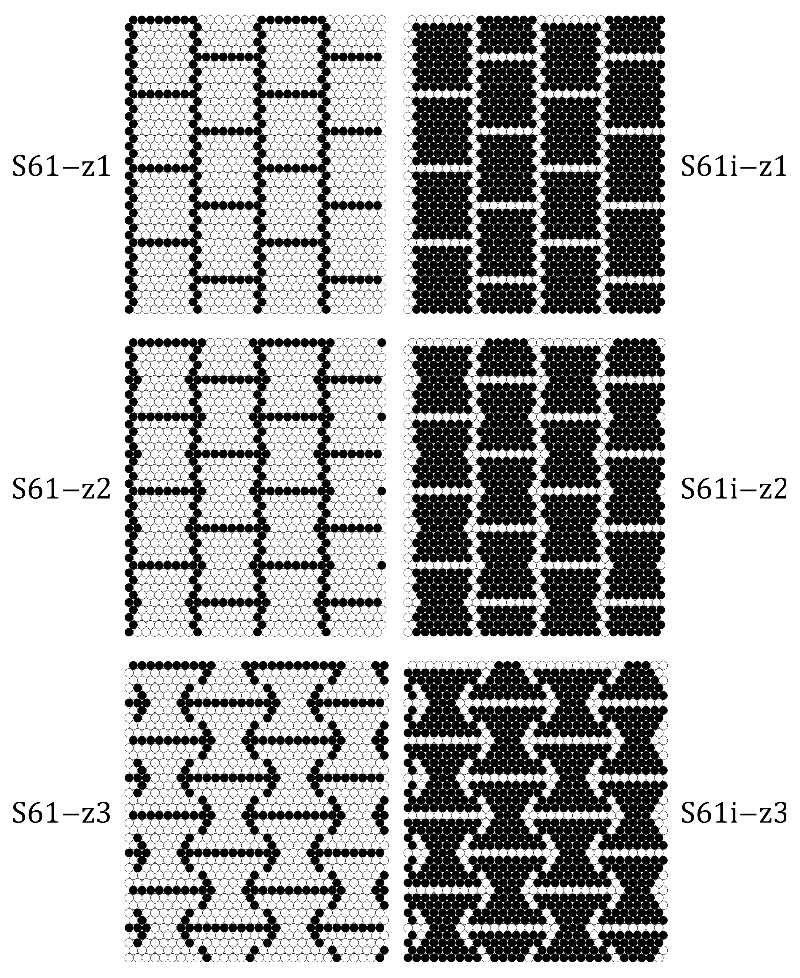
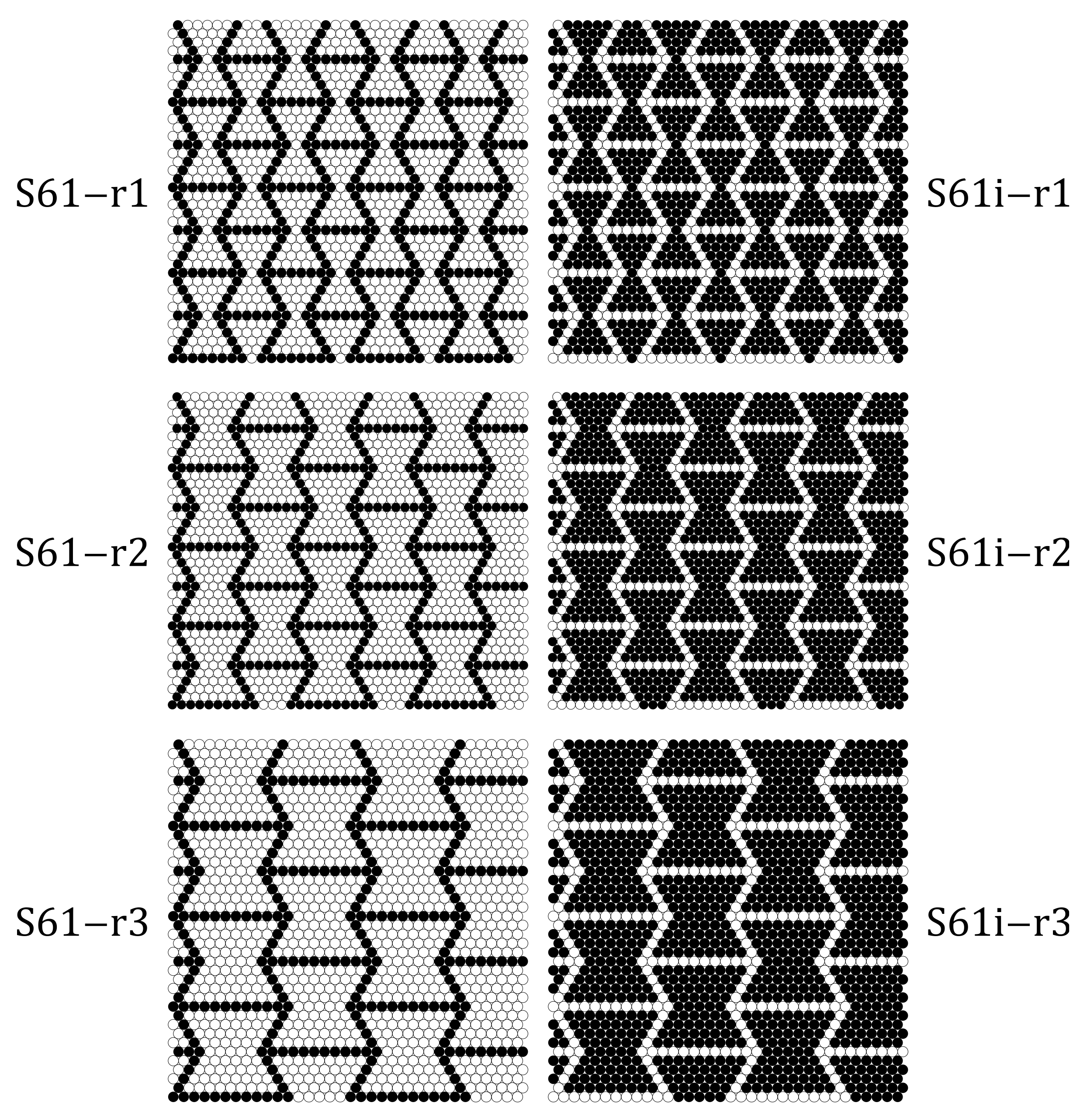
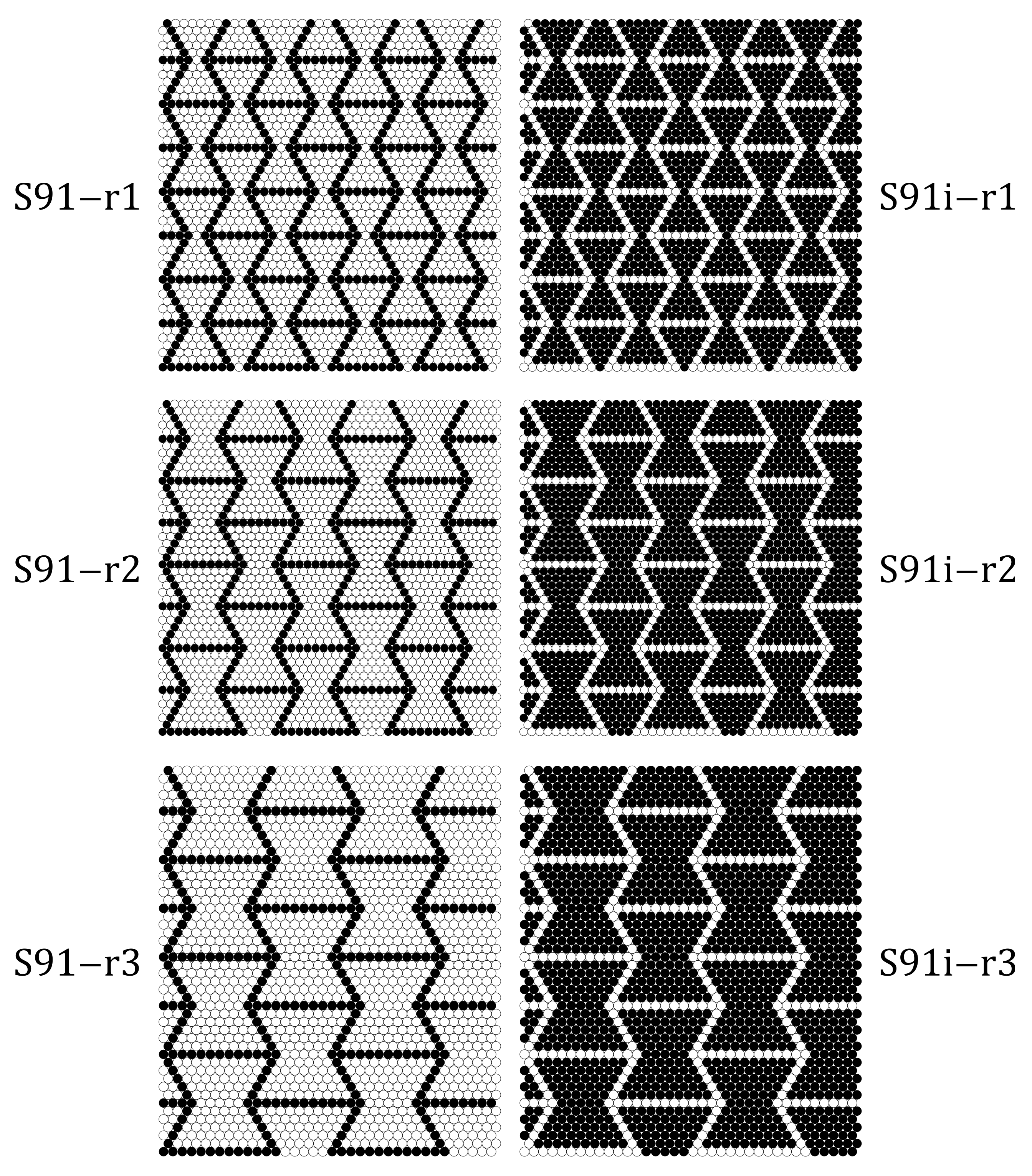
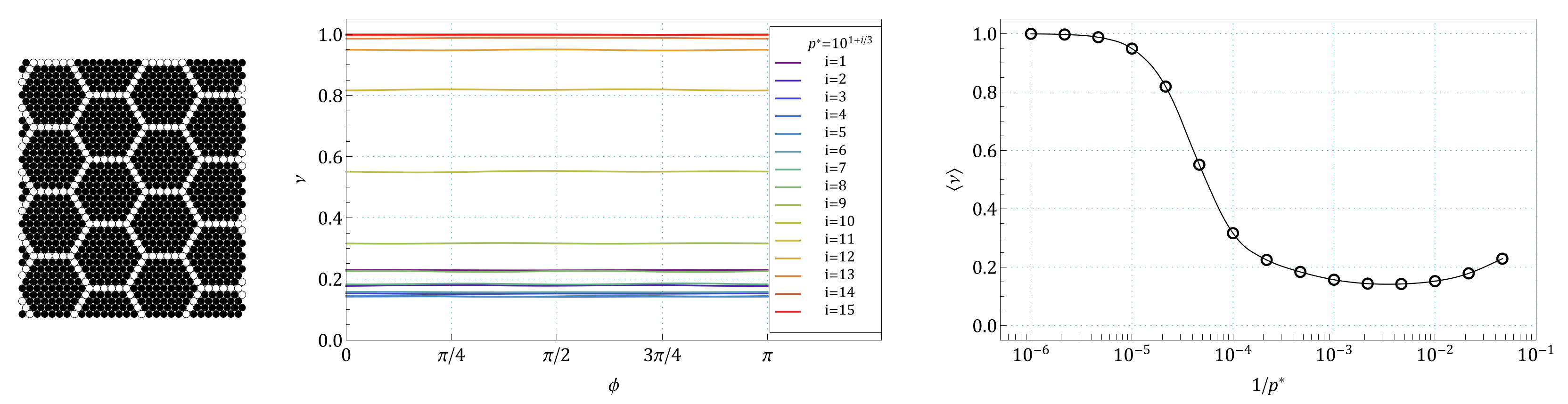
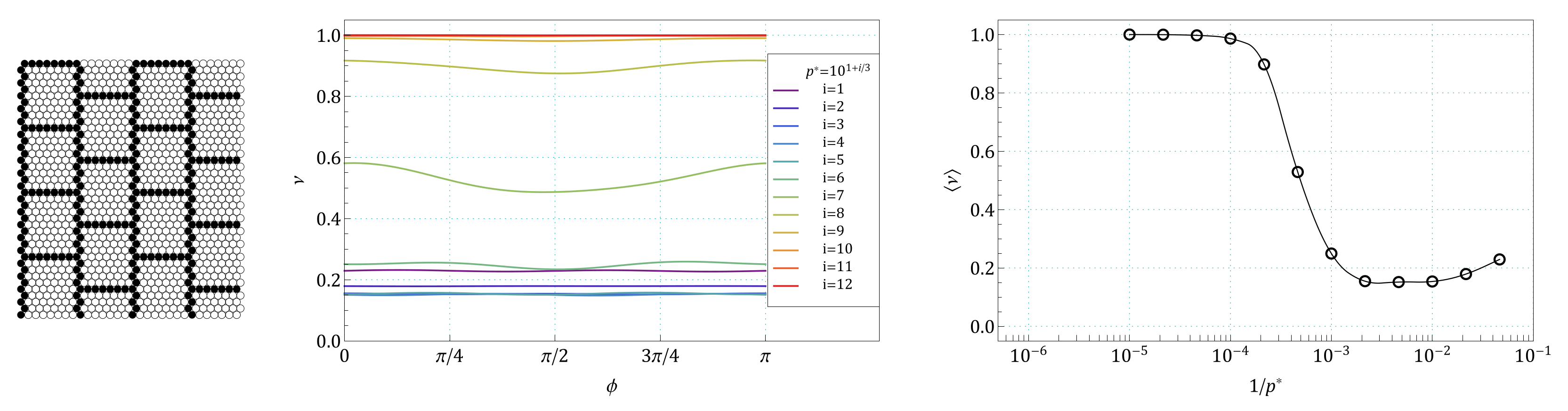
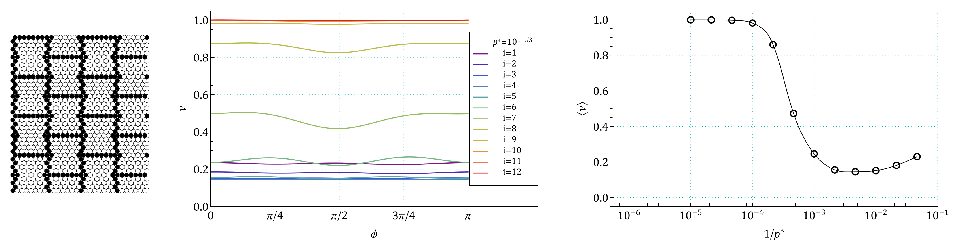
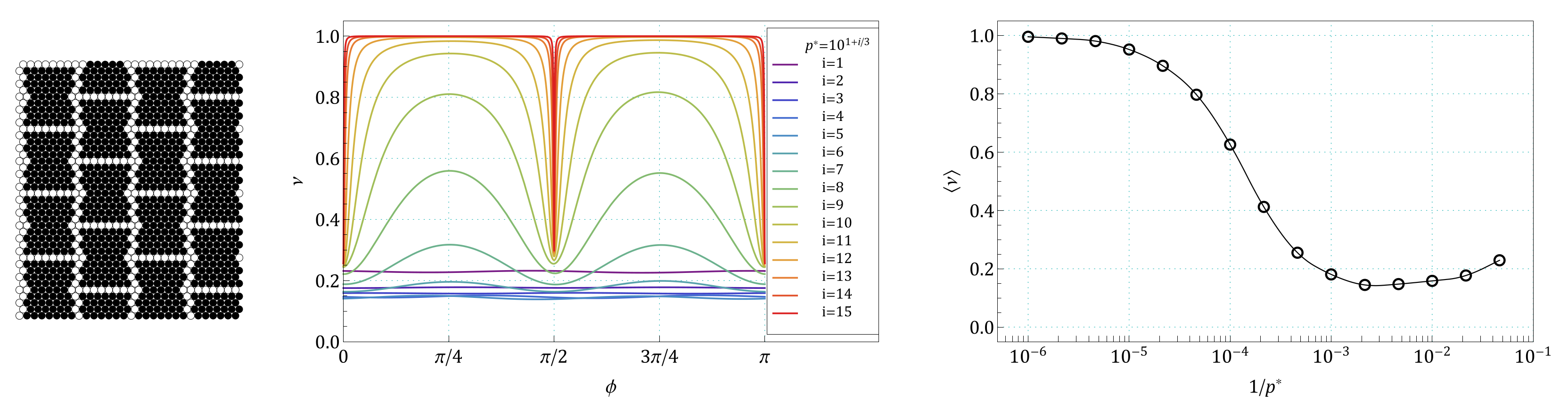
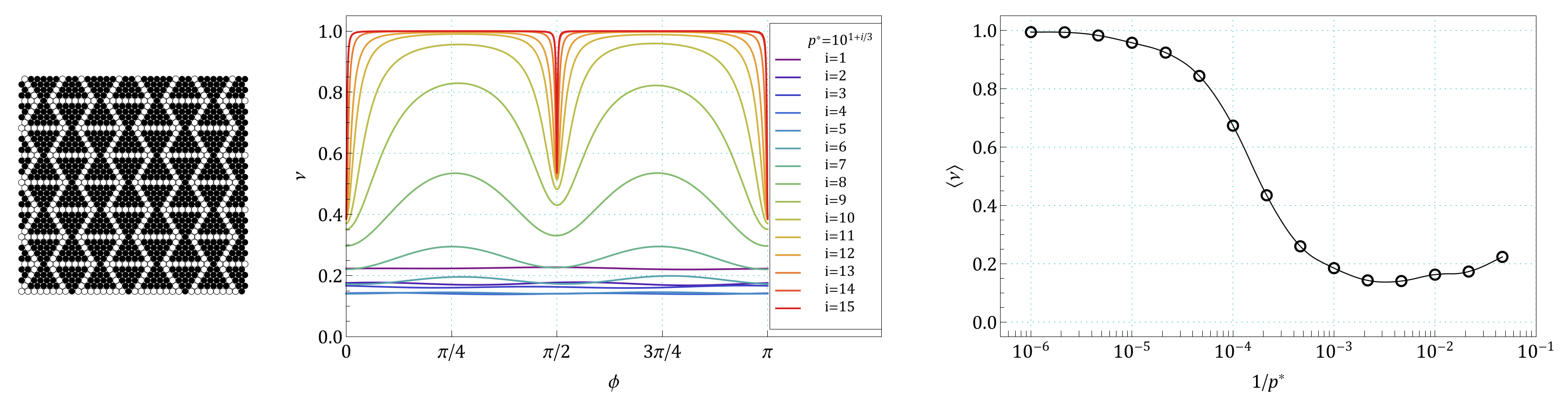
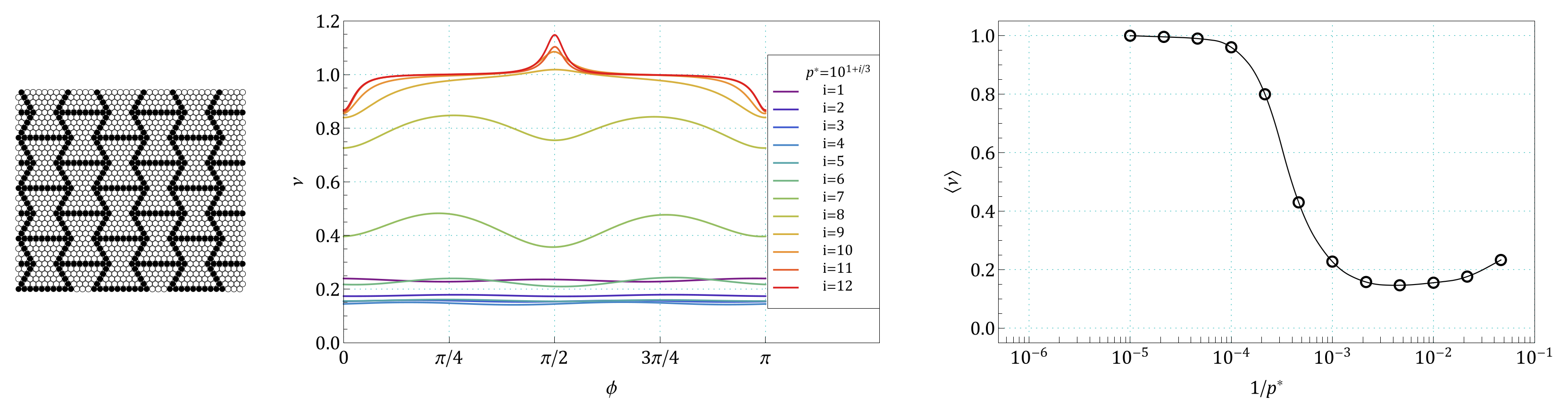
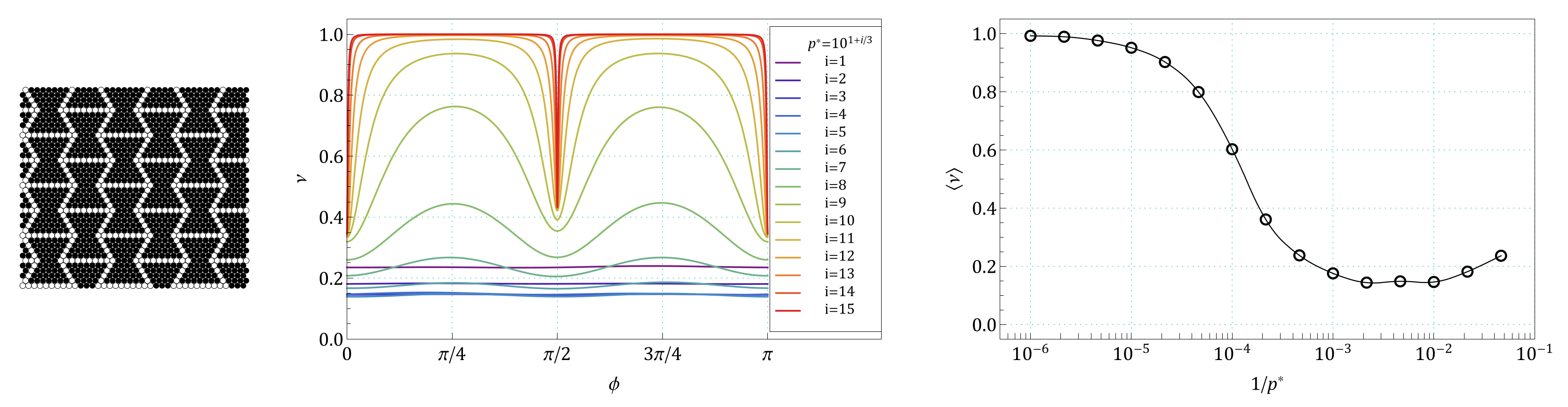
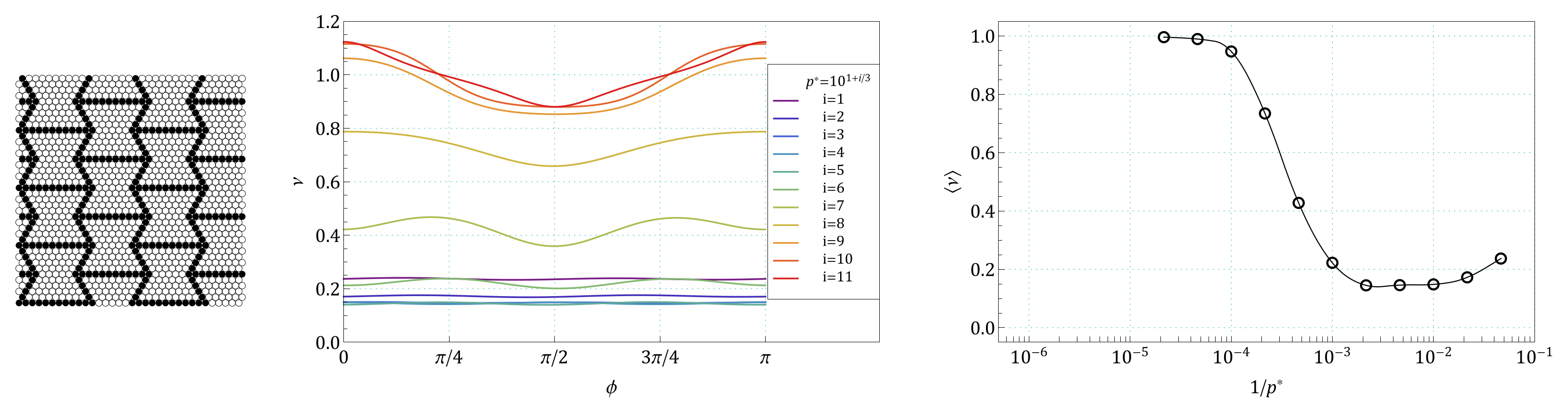
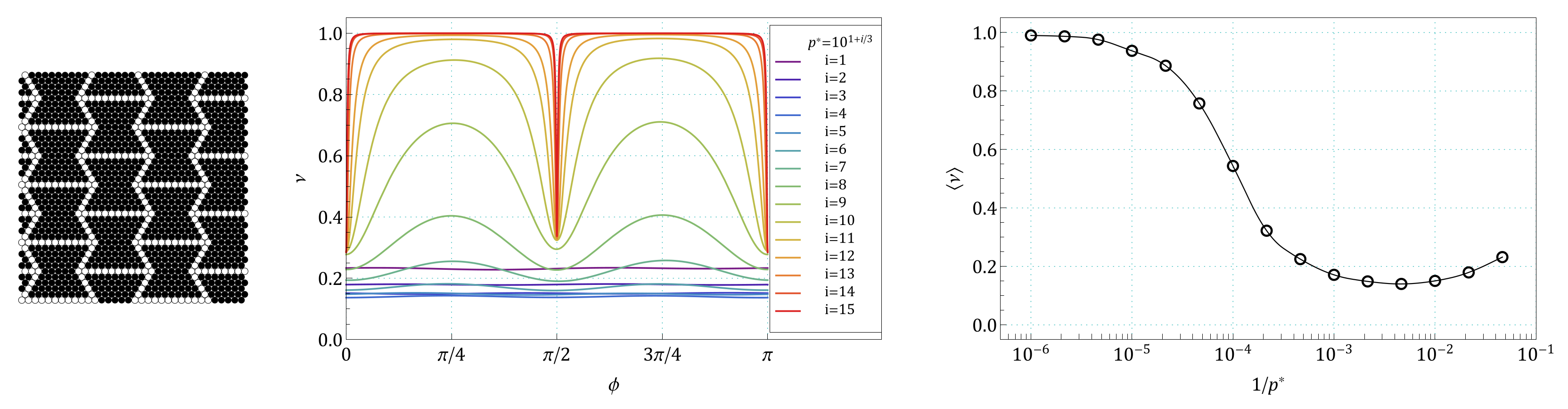
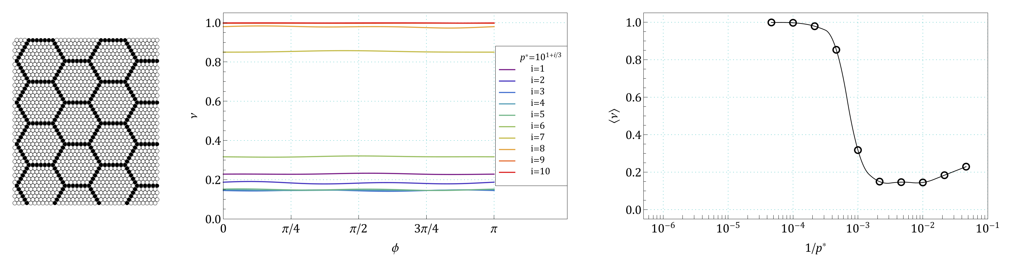
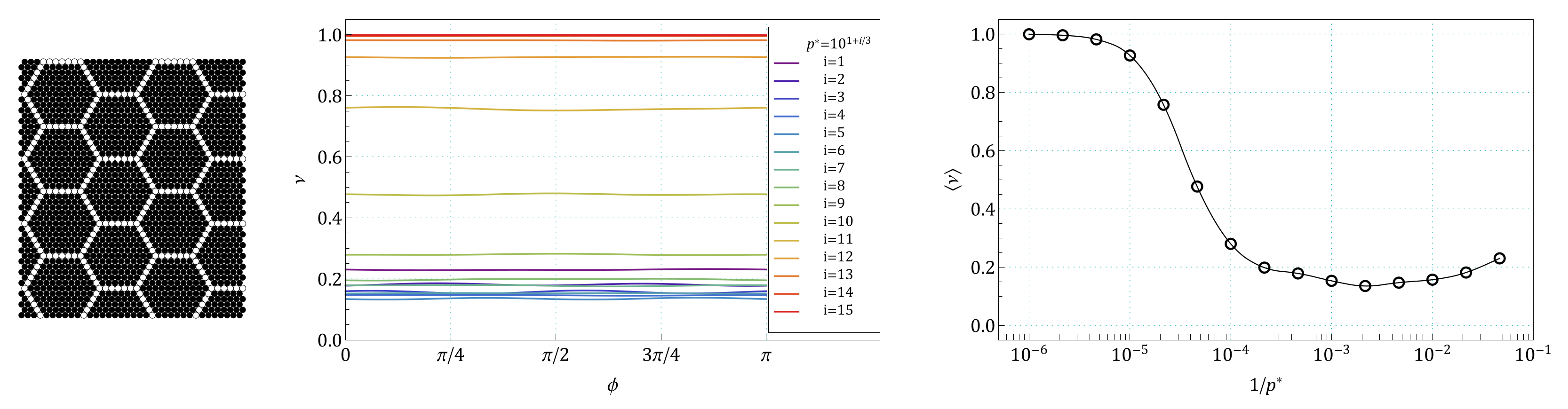
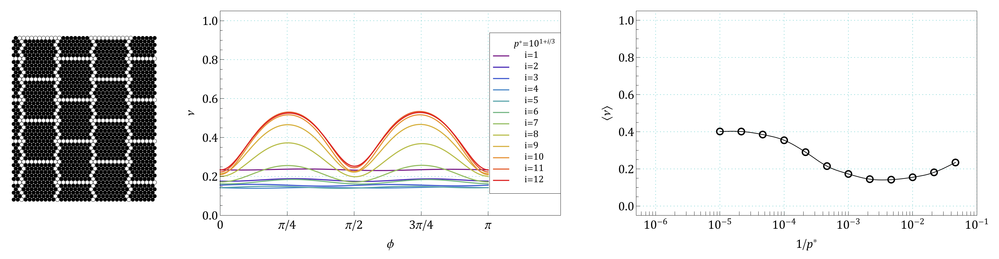
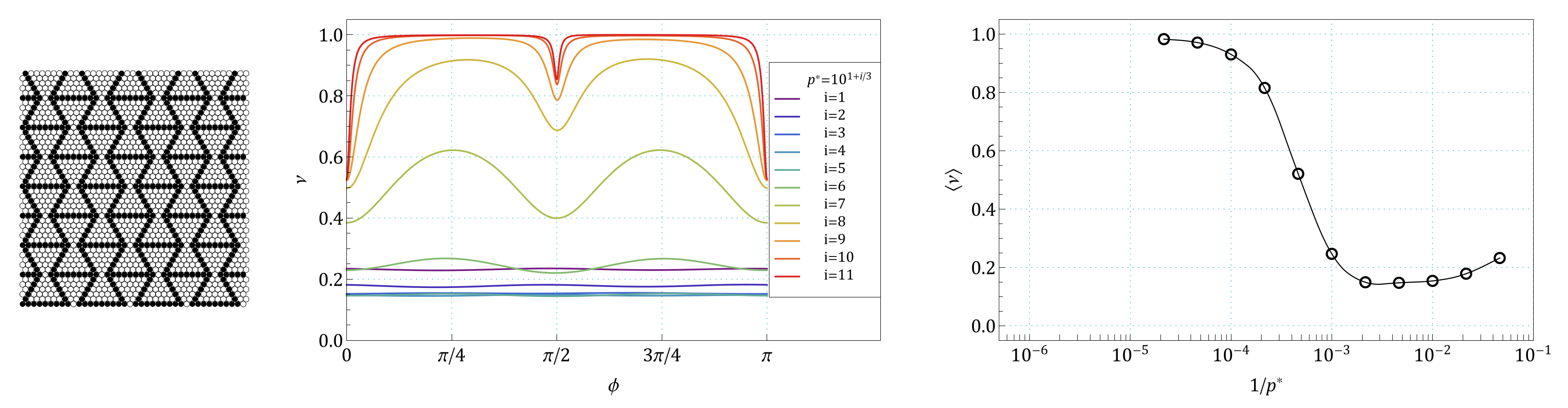
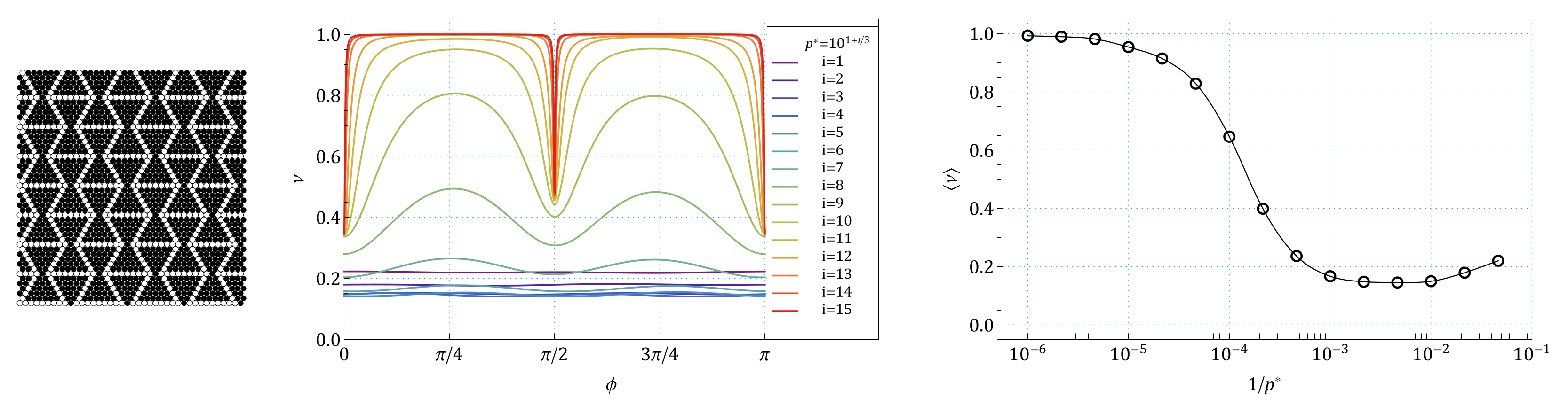
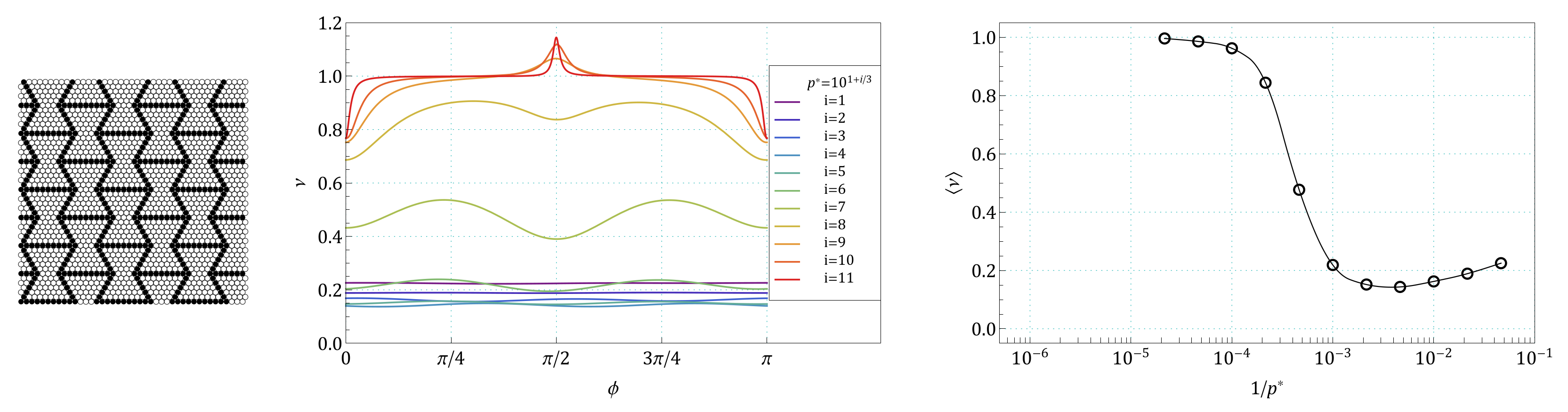
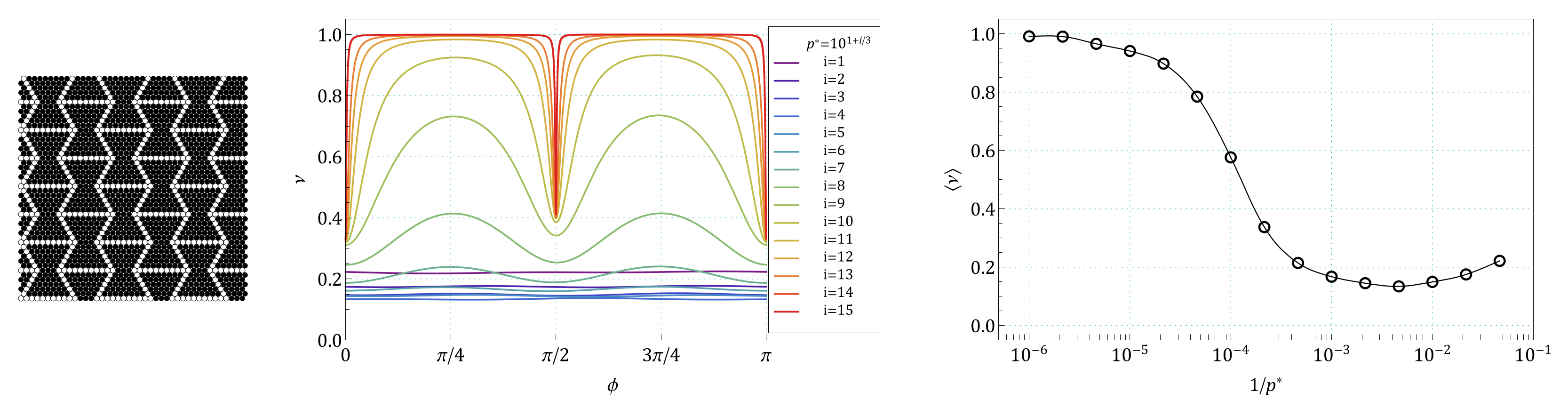
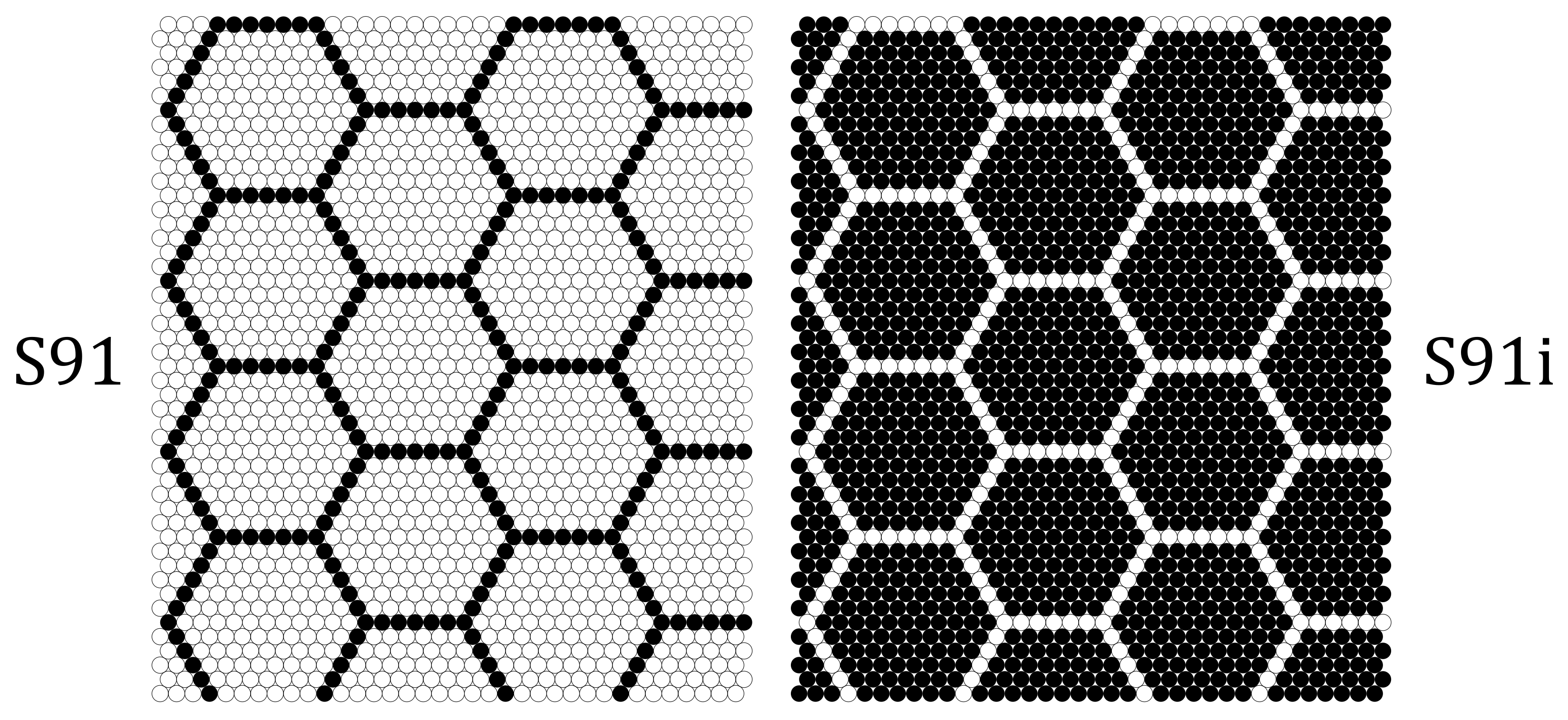
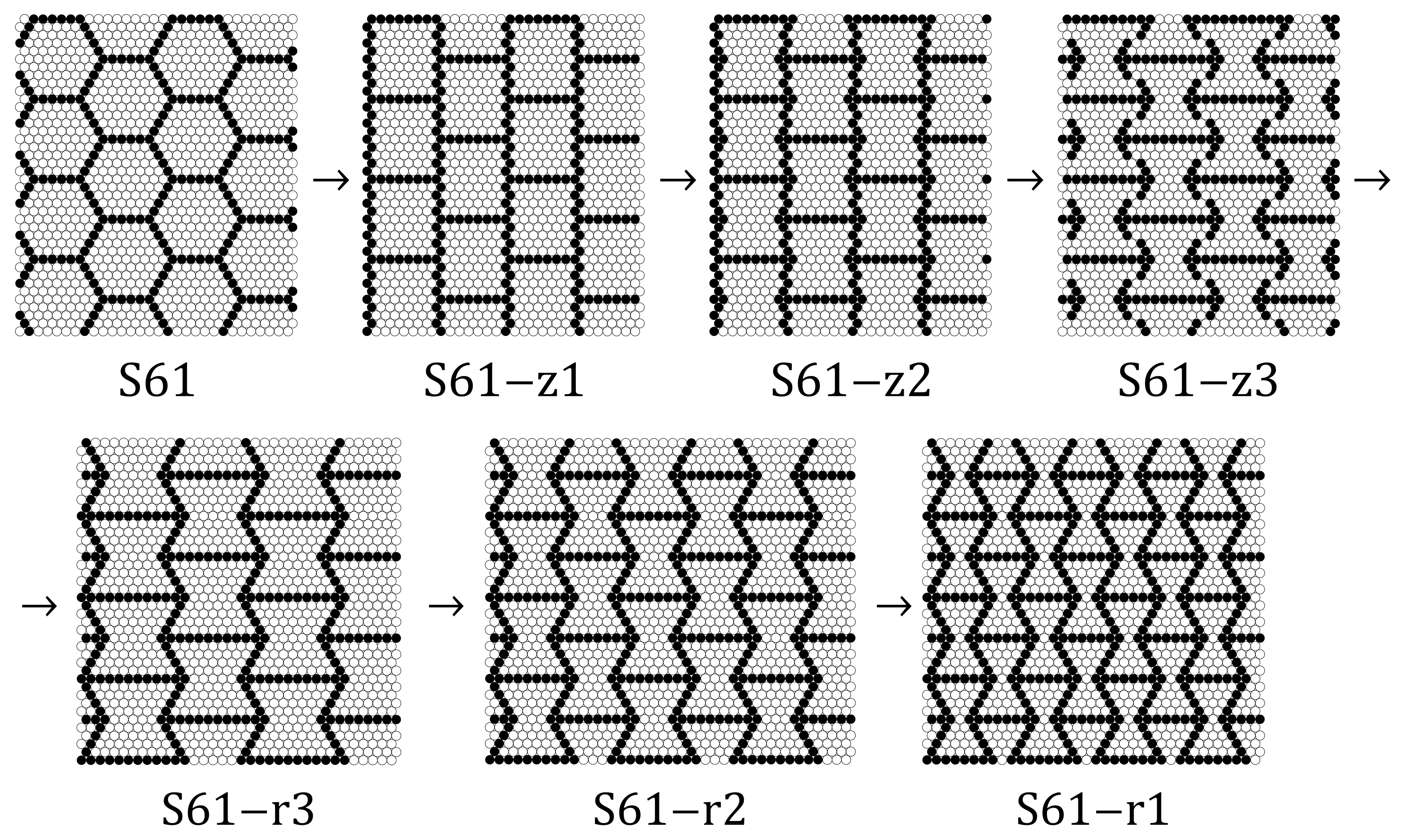
Appendix A. Images of Modified S61 and S91 Structures, Studied in the Work

In this appendix the structures which were not defined in the main part of this paper are presented. The structure names are explained in figure captions.
Figure A1. Images of S61-zk (left) and S61i-zk (right) “zigzag” binary disc systems with an anisotropic pattern of two-fold symmetry. Black dots and open circles represent the HD of various sizes: “large” (with a diameter equal to ( 1 + δ ) σ ) and “small” (with a diameter equal to ( 1 δ ) σ ), respectively. The numbers k = 1 , 2 , 3 after ‘z’ indicate how many atoms have been added to each side of any horizontal “line” forming the frame of the base (S61 or S61i) structure.
Symmetry 13 01127 g0a1
Figure A2. Images of S61-rk (left) and S61i-rk (right) “re-entrant” binary disc systems with an anisotropic pattern of two-fold symmetry. Black dots and open circles represent the HD of various sizes: “large” (with a diameter equal to ( 1 + δ ) σ ) and “small” (with a diameter equal to ( 1 δ ) σ ), respectively. The numbers k = 1 , 2 , 3 after ‘r’ indicate how many atoms have been added to each side of any horizontal “line” forming the frame of the base (S61 or S61i) structure.
Symmetry 13 01127 g0a2
Figure A3. Images of S91-zk (left) and S91i-zk (right) “zigzag” binary disc systems with an anisotropic pattern of two-fold symmetry. Black dots and open circles represent the HD of various sizes: “large” (with a diameter equal to ( 1 + δ ) σ ) and “small” (with a diameter equal to ( 1 δ ) σ ), respectively. The numbers k = 1 , 2 after ‘z’ indicate how many atoms have been added to each side of any horizontal “line” forming the frame of the base (S91 or S91i) structure.
Symmetry 13 01127 g0a3
Figure A4. Images of S91-rk (left) and S91i-rk (right) “re-entrant” binary disc systems with an anisotropic pattern of two-fold symmetry. Black dots and open circles represent the HD of various sizes: “large” (with a diameter equal to ( 1 + δ ) σ ) and “small” (with a diameter equal to ( 1 δ ) σ ), respectively. The numbers k = 1 , 2 , 3 after ‘r’ indicate how many atoms have been added to each side of any horizontal “line” forming the frame of the base (S91 or S91i) structure.
Symmetry 13 01127 g0a4

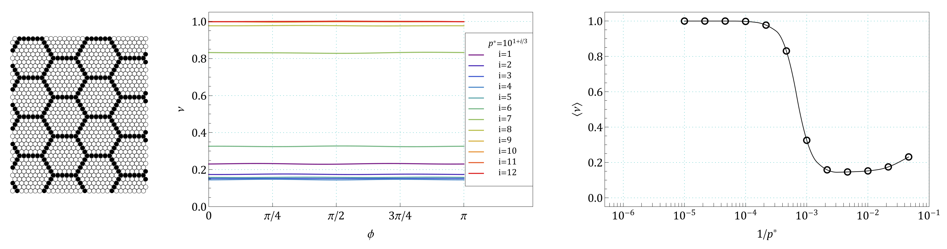
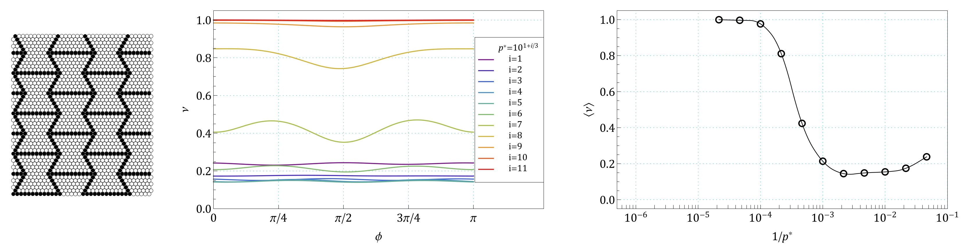
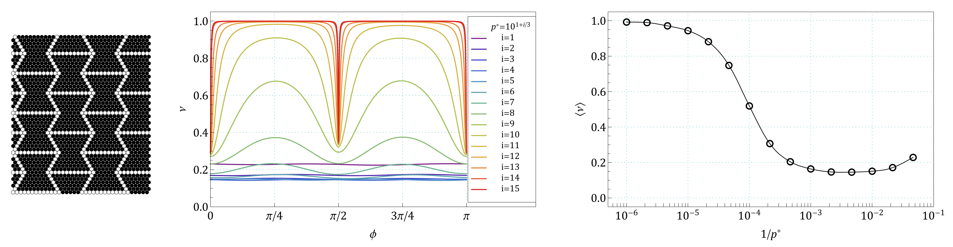
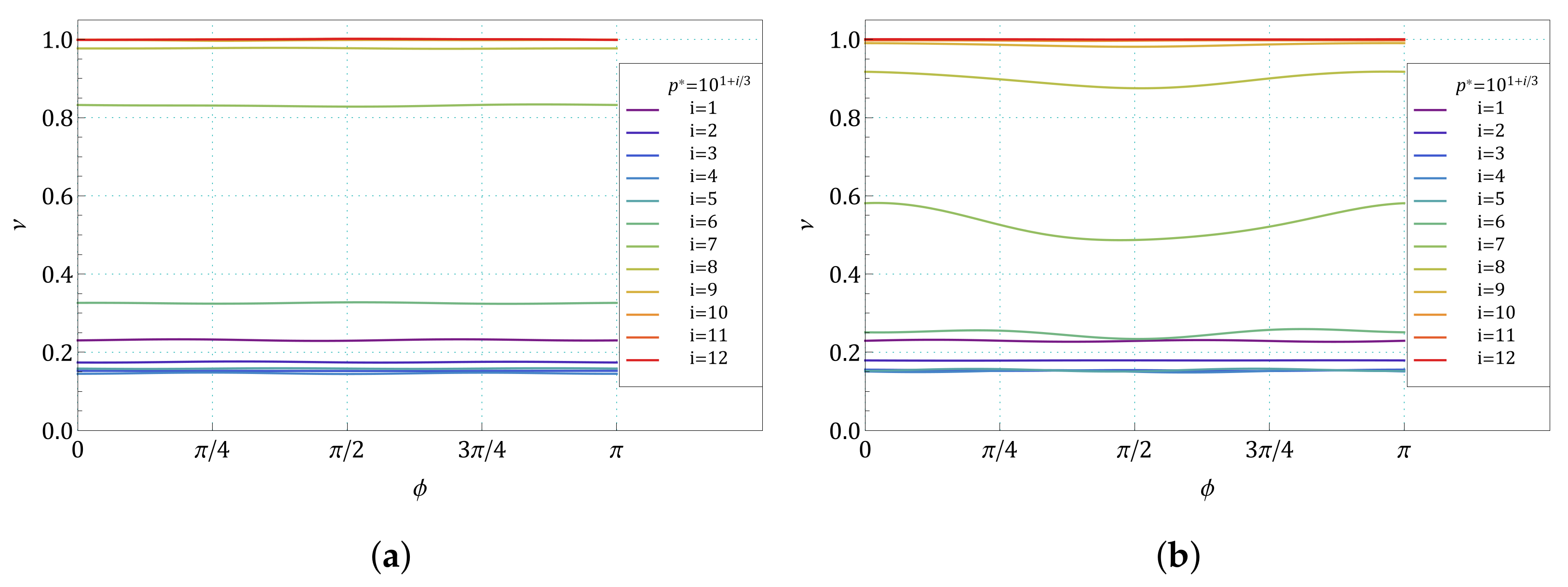
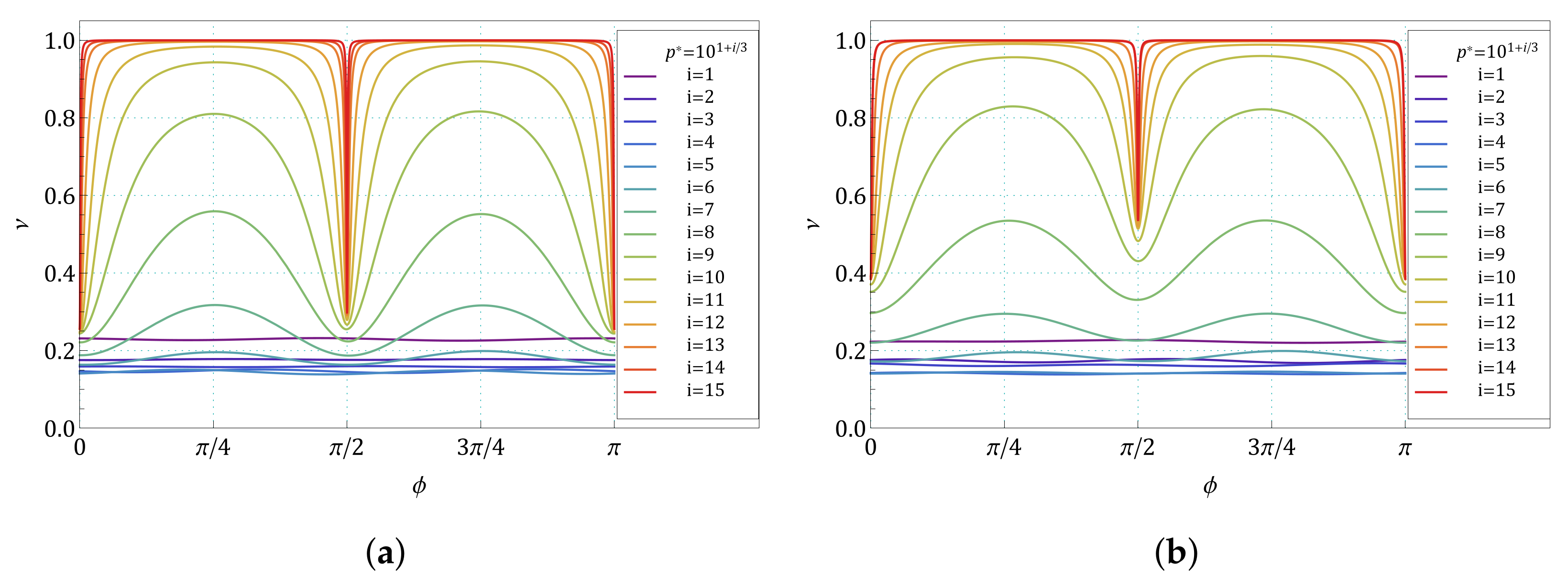
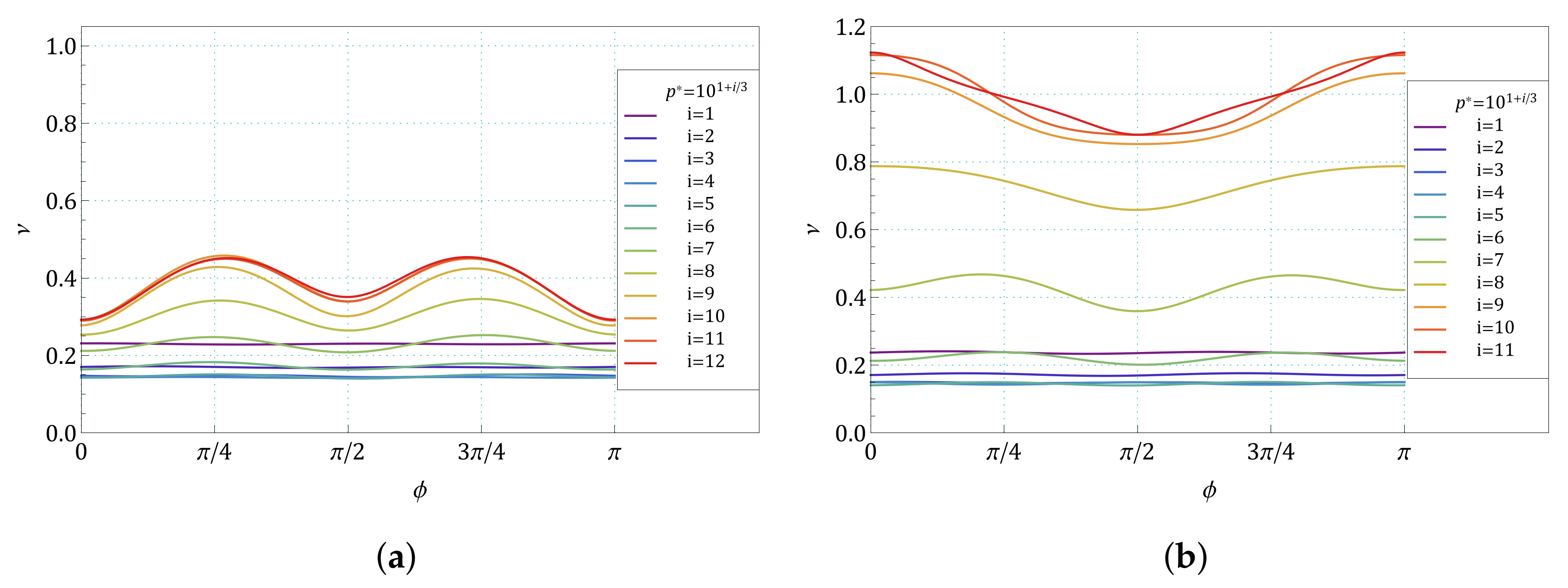
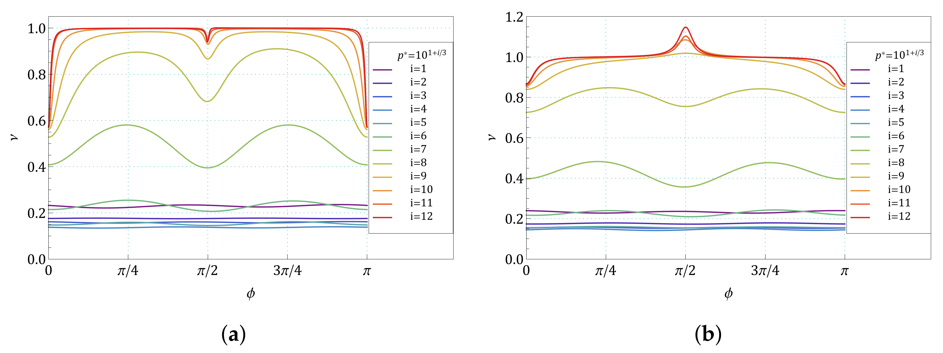
Appendix B. The Summary of Angle Dependence of Poisson’s Ratio, ν(ϕ), and Pressure Dependence of Average Value of Poisson’s Ratio, 〈ν(1/p*)〉, for All Pressures and for All the Structures Studied in the Work

For the convenience of the reader the results are presented for all structures studied and are arranged in three columns. In the 1 st column the structure geometry is shown, and in the 2 nd and the 3 rd , respectively, the angular dependence and pressure dependence are plotted.
Figure A5. Image of structure S61 (left) and its dependencies: ν ( ϕ ) (center) and ν ( 1 / p ) (right).
Symmetry 13 01127 g0a5
Figure A6. Image of structure S61i (left) and its dependencies: ν ( ϕ ) (center) and ν ( 1 / p ) (right).
Symmetry 13 01127 g0a6
Figure A7. Image of structure S61-z1 (left) and its dependencies: ν ( ϕ ) (center) and ν ( 1 / p ) (right). The length of the simulation for the four highest pressures was equal to 4 × 10 7 cycles.
Symmetry 13 01127 g0a7
Figure A8. Image of structure S61i-z1 (left) and its dependencies: ν ( ϕ ) (center) and ν ( 1 / p ) (right). The length of the simulation for the three highest pressures was equal to 4 × 10 7 cycles.
Symmetry 13 01127 g0a8
Figure A9. Image of structure S61-z2 (left) and its dependencies: ν ( ϕ ) (center) and ν ( 1 / p ) (right). The length of the simulation for the four highest pressures was equal to 4 × 10 7 cycles.
Symmetry 13 01127 g0a9
Figure A10. Image of structure S61i-z2 (left) and its dependencies: ν ( ϕ ) (center) and ν ( 1 / p ) (right). The length of the simulation for the three highest pressures was equal to 4 × 10 7 cycles.
Symmetry 13 01127 g0a10
Figure A11. Image of structure S61-z3 (left) and its dependencies: ν ( ϕ ) (center) and ν ( 1 / p ) (right). The length of the simulation for the five highest pressures was equal to 4 × 10 7 cycles.
Symmetry 13 01127 g0a11
Figure A12. Image of structure S61i-z3 (left) and its dependencies: ν ( ϕ ) (center) and ν ( 1 / p ) (right). The length of the simulation for the two highest pressures was equal to 4 × 10 7 cycles.
Symmetry 13 01127 g0a12
Figure A13. Image of structure S61-r1 (left) and its dependencies: ν ( ϕ ) (center) and ν ( 1 / p ) (right). The length of the simulation for the four highest pressures was equal to 17 × 10 7 cycles.
Symmetry 13 01127 g0a13
Figure A14. Image of structure S61i-r1 (left) and its dependencies: ν ( ϕ ) (center) and ν ( 1 / p ) (right). The length of the simulation for the three highest pressures was equal to 4 × 10 7 cycles.
Symmetry 13 01127 g0a14
Figure A15. Image of structure S61-r2 (left) and its dependencies: ν ( ϕ ) (center) and ν ( 1 / p ) (right). The length of the simulation for the four highest pressures was equal to 17 × 10 7 cycles.
Symmetry 13 01127 g0a15
Figure A16. Image of structure S61i-r2 (left) and its dependencies: ν ( ϕ ) (center) and ν ( 1 / p ) (right). The length of the simulation for the three highest pressures was equal to 4 × 10 7 cycles.
Symmetry 13 01127 g0a16
Figure A17. Image of structure S61-r3 (left) and its dependencies: ν ( ϕ ) (center) and ν ( 1 / p ) (right). The length of the simulation for the three highest pressures was equal to 17 × 10 7 cycles.
Symmetry 13 01127 g0a17
Figure A18. Image of structure S61i-r3 (left) and its dependencies: ν ( ϕ ) (center) and ν ( 1 / p ) (right). The length of the simulation for the three highest pressures was equal to 4 × 10 7 cycles.
Symmetry 13 01127 g0a18
Figure A19. Image of structure S91 (left) and its dependencies: ν ( ϕ ) (center) and ν ( 1 / p ) (right). The length of the simulation for the two highest pressures was equal to 17 × 10 7 cycles.
Symmetry 13 01127 g0a19
Figure A20. Image of structure S91i (left) and its dependencies: ν ( ϕ ) (center) and ν ( 1 / p ) (right). The length of the simulation for the four highest pressures was equal to 17 × 10 7 cycles.
Symmetry 13 01127 g0a20
Figure A21. Image of structure S91-z1 (left) and its dependencies: ν ( ϕ ) (center) and ν ( 1 / p ) (right). The length of the simulation for the four highest pressures was equal to 4 × 10 7 cycles.
Symmetry 13 01127 g0a21
Figure A22. Image of structure S91i-z1 (left) and its dependencies: ν ( ϕ ) (center) and ν ( 1 / p ) (right). The length of the simulation for the three highest pressures was equal to 4 × 10 7 cycles.
Symmetry 13 01127 g0a22
Figure A23. Image of structure S91-z2 (left) and its dependencies: ν ( ϕ ) (center) and ν ( 1 / p ) (right). The length of the simulation for the four highest pressures was equal to 4 × 10 7 cycles.
Symmetry 13 01127 g0a23
Figure A24. Image of structure S91i-z2 (left) and its dependencies: ν ( ϕ ) (center) and ν ( 1 / p ) (right).
Symmetry 13 01127 g0a24
Figure A25. Image of structure S91-r1 (left) and its dependencies: ν ( ϕ ) (center) and ν ( 1 / p ) (right). The length of the simulation for the three highest pressures was equal to 17 × 10 7 cycles.
Symmetry 13 01127 g0a25
Figure A26. Image of structure S91i-r1 (left) and its dependencies: ν ( ϕ ) (center) and ν ( 1 / p ) (right). The length of the simulation for the three highest pressures was equal to 4 × 10 7 cycles.
Symmetry 13 01127 g0a26
Figure A27. Image of structure S91-r2 (left) and its dependencies: ν ( ϕ ) (center) and ν ( 1 / p ) (right). The length of the simulation for the three highest pressures was equal to 17 × 10 7 cycles.
Symmetry 13 01127 g0a27
Figure A28. Image of structure S91i-r2 (left) and its dependencies: ν ( ϕ ) (center) and ν ( 1 / p ) (right). The length of the simulation for the three highest pressures was equal to 4 × 10 7 cycles.
Symmetry 13 01127 g0a28
Figure A29. Image of structure S91-r3 (left) and its dependencies: ν ( ϕ ) (center) and ν ( 1 / p ) (right). The length of the simulation for the three highest pressures was equal to 17 × 10 7 cycles.
Symmetry 13 01127 g0a29
Figure A30. Image of structure S91i-r3 (left) and its dependencies: ν ( ϕ ) (center) and ν ( 1 / p ) (right). The length of the simulation for the three highest pressures was equal to 4 × 10 7 cycles.
Symmetry 13 01127 g0a30

References

  1. Landau, L.; Lifshits, E. Theory of Elasticity, 3rd ed.; Pergamon Press: Oxford, UK, 1993. [Google Scholar]
  2. Wojciechowski, K.W. Negative Poisson ratios at negative pressures. Mol. Phys. Rep. 1995, 10, 129–136. [Google Scholar]
  3. Wojciechowski, K.W. Remarks on “Poisson Ratio beyond the Limits of the Elasticity Theory”. J. Phys. Soc. Jpn. 2003, 72, 1819–1820. [Google Scholar] [CrossRef]
  4. Tretiakov, K.V.; Bilski, M.; Wojciechowski, K.W. Maximum Poisson’s Ratios in Planar Isotropic Crystals of Binary Hard Discs at High Pressures. Phys. Status Solidi B 2017, 254, 1700543. [Google Scholar] [CrossRef]
  5. Strek, T.; Jopek, H.; Nienartowicz, M. Dynamic response of sandwich panels with auxetic cores. Phys. Status Solidi B 2015, 252, 1540–1550. [Google Scholar] [CrossRef]
  6. Mizzi, L.; Grima, J.N.; Gatt, R.; Attard, D. Analysis of the Deformation Behavior and Mechanical Properties of Slit-Perforated Auxetic Metamaterials. Phys. Status Solidi B 2019, 256, 1800153. [Google Scholar] [CrossRef] [Green Version]
  7. Zulifqar, A.; Hu, H. Development of Bi-Stretch Auxetic Woven Fabrics Based on Re-Entrant Hexagonal Geometry. Phys. Status Solidi B 2019, 256, 1800172. [Google Scholar] [CrossRef] [Green Version]
  8. Almgren, R.F. An isotropic three-dimensional structure with Poisson’s ratio =−1. J. Elast. 1985, 15, 427–430. [Google Scholar]
  9. Lakes, R.S. Foam Structures with a Negative Poisson’s Ratio. Science 1987, 235, 1038–1040. [Google Scholar] [CrossRef]
  10. Wojciechowski, K.W. Constant thermodynamic tension Monte Carlo studies of elastic properties of a two-dimensional system of hard cyclic hexamers. Mol. Phys. 1987, 61, 1247–1258. [Google Scholar] [CrossRef]
  11. Gibson, L.J.; Ashby, M.F. Cellular Solids: Structure and Properties; Pergamon Press: Oxford, UK, 1988. [Google Scholar]
  12. Wojciechowski, K.W. Two-dimensional Isotropic System with a Negative Poisson Ratio. Phys. Lett. A 1989, 137, 60–64. [Google Scholar] [CrossRef]
  13. Evans, K.E. Auxetic polymers: A new range of materials. Endeavour 1991, 15, 170–174. [Google Scholar] [CrossRef]
  14. Grima, J.N.; Evans, K.E. Auxetic behavior from rotating squares. J. Mat. Sci. Lett. 2000, 19, 1563–1565. [Google Scholar] [CrossRef]
  15. Tretiakov, K.V. Negative Poisson’s ratio of two-dimensional hard cyclic tetramers. J. Non-Cryst. Solids 2009, 355, 24–27. [Google Scholar] [CrossRef]
  16. Fowler, P.W.; Guest, S.D.; Tarnai, T. Symmetry Perspectives on Some Auxetic Body-Bar Frameworks. Symmetry 2014, 6, 368–382. [Google Scholar] [CrossRef] [Green Version]
  17. Wang, Y.C.; Lai, H.W.; Ren, X.J. Enhanced Auxetic and Viscoelastic Properties of Filled Reentrant Honeycomb. Phys. Status Solidi B 2020, 257, 1900184. [Google Scholar] [CrossRef]
  18. Lim, T.C. An Auxetic System Based on Interconnected Y-Elements Inspired by Islamic Geometric Patterns. Symmetry 2021, 13, 865. [Google Scholar] [CrossRef]
  19. Lakes, R. Advances in negative Poisson’s ratio materials. Adv. Mater. 1993, 5, 293–296. [Google Scholar] [CrossRef]
  20. Prawoto, Y. Seeing auxetic materials from the mechanics point of view: A structural review on the negative Poisson’s ratio. Comp. Mater. Sci. 2012, 58, 140–153. [Google Scholar] [CrossRef]
  21. Mizzi, L.; Attard, D.; Casha, A.; Grima, J.N.; Gatt, R. On the suitability of hexagonal honeycombs as stent geometries. Phys. Status Solidi B 2014, 251, 328–337. [Google Scholar] [CrossRef]
  22. Allen, T.; Hewage, T.; Newton-Mann, C.; Wang, W.; Duncan, O.; Alderson, A. Fabrication of auxetic foam sheets for sports applications. Phys. Status Solidi B 2017, 254, 1700596. [Google Scholar] [CrossRef] [Green Version]
  23. Ren, X.; Das, R.; Tran, P.; Ngo, T.D.; Xie, Y.M. Auxetic metamaterials and structures: A review. Smart Mater. Struct. 2018, 27, 023001. [Google Scholar] [CrossRef]
  24. Wang, Y.B.; Sotzing, G.A.; Weiss, R.A. Conductive Polymer Foams as Sensors for Volatile Amines. Chem. Mater. 2003, 15, 375–377. [Google Scholar] [CrossRef]
  25. Chen, Y.J.; Li, Y.; Chu, B.T.T.; Kuo, I.T.; Yip, M.C.; Tai, N. Porous composites coated with hybrid nano carbon materials perform excellent electromagnetic interference shielding. Compos. Part B 2015, 70, 231–237. [Google Scholar] [CrossRef]
  26. Zhang, X.C.; Scarpa, F.; McHale, R.; Limmack, A.P.; Peng, H.X. Carbon nano-ink coated open cell polyurethane foam with micro-architectured multilayer skeleton for damping applications. RSC Adv. 2016, 6, 80334–80341. [Google Scholar] [CrossRef] [Green Version]
  27. Duncan, O.; Shepherd, T.; Moroney, C.; Foster, L.; Venkatraman, P.D.; Winwood, K.; Allen, T.; Alderson, A. Review of auxetic materials for sports applications: Expanding options in comfort and protection. Appl. Sci. Basel 2018, 8, 941. [Google Scholar] [CrossRef] [Green Version]
  28. Grima-Cornish, J.N.; Cauchi, R.; Attard, D.; Gatt, R.; Grima, J.N. Smart Honeycomb “Mechanical Metamaterials” with Tunable Poisson’s Ratios. Phys. Status Solidi B 2020, 257, 1900707. [Google Scholar] [CrossRef]
  29. Brańka, A.C.; Pierański, P.; Wojciechowski, K.W. Rotatory phase in a system of hard cyclic hexamers; an experimental modelling study. J. Phys. Chem. Solids 1982, 43, 817–818. [Google Scholar] [CrossRef]
  30. Wojciechowski, K.W. Monte Carlo simulations of highly anisotropic two-dimensional hard dumbbell-shaped molecules: Nonperiodic phase between fluid and dense solid. Phys. Rev. B 1992, 46, 26–39. [Google Scholar] [CrossRef] [PubMed]
  31. Allen, M.P.; Evans, G.T.; Frenkel, D.; Mulder, B.M. Hard Convex Body Fluids. Adv. Chem. Phys. 1993, 86, 1–166. [Google Scholar]
  32. Weeks, J.D.; Chandler, D.; Andersen, H.C. Perturbation Theory of the Thermody-namic Properties of Simple Liquids. J. Chem. Phys. 1971, 55, 5422. [Google Scholar] [CrossRef]
  33. Frenkel, D. Order through entropy. Nat. Mater. 2015, 14, 9–12. [Google Scholar] [CrossRef]
  34. Aoki, K.M.; Ito, N. Effect of size polydispersity on granular materials. Phys. Rev. E 1996, 54, 1990–1996. [Google Scholar] [CrossRef]
  35. Both, J.A.; Hong, D.C. Variational Approach to Hard Sphere Segregation under Gravity. Phys. Rev. Lett. 2002, 88, 124301. [Google Scholar] [CrossRef] [Green Version]
  36. Parrinello, M.; Rahman, A. Strain fluctuations and elastic constants. J. Chem. Phys. 1982, 76, 2662–2666. [Google Scholar] [CrossRef]
  37. Ray, J.R.; Rahman, A. Statistical ensembles and molecular dynamics studies of anisotropic solids. J. Chem. Phys. 1984, 80, 4423–4426. [Google Scholar] [CrossRef]
  38. Wojciechowski, K.W.; Tretiakov, K.V.; Kowalik, M. Elastic properties of dense solid phases of hard cyclic pentamers and heptamers in two dimensions. Phys. Rev. E 2003, 67, 036121. [Google Scholar] [CrossRef] [Green Version]
  39. Tokmakova, S.P. Stereographic projections of Poisson’s ratio in auxetic crystals. Phys. Status Solidi B 2005, 242, 721–729. [Google Scholar] [CrossRef]
  40. Bilski, M.; Wojciechowski, K.W. Tailoring Poisson’s ratio by introducing auxetic layers. Phys. Status Solidi B 2016, 253, 1318–1323. [Google Scholar] [CrossRef]
  41. Wojciechowski, K.W.; Tretiakov, K.V.; Brańka, A.C.; Kowalik, M. Elastic properties of two-dimensional hard discs in the close-packing limit. J. Chem. Phys. 2003, 119, 939–946. [Google Scholar] [CrossRef]
Figure 1. Images of S61 (left) and S61i (right) binary disc systems with an isotropic pattern of six-fold symmetry. The value ‘61’ comes from the number of “white” (on the left) or “black” (on the right) atoms inside a “frame” made of “black” or “white” atoms, respectively. Black dots and open circles represent the HD of various sizes: “large” (with a diameter equal to ( 1 + δ ) σ ) and “small” (with a diameter equal to ( 1 δ ) σ ), respectively.
Symmetry 13 01127 g001
Figure 2. Images of S91 (left) and S91i (right) binary disc systems with an isotropic pattern of six-fold symmetry. The value ‘91’ comes from the number of “white” (on the left) or “black” (on the right) atoms inside a “frame” made of “black” or “white” atoms, respectively. Black dots and open circles represent the HD of various sizes: “large” (with a diameter equal to ( 1 + δ ) σ ) and “small” (with a diameter equal to ( 1 δ ) σ ), respectively.
Symmetry 13 01127 g002
Figure 3. Example transition from honeycomb-based S61 structure (isotropic, with six-fold symmetry) to re-entrant (r) structures (anisotropic, with two-fold symmetry). Transition structures are called “zigzag” (z) structures, due to the shapes of their vertical sides.
Symmetry 13 01127 g003
Figure 4. Average components of the simulation box of the system, h i j , for S91 at reduced pressure p = 10 5 . The averages were calculated basing on short excerpts from the MC simulation (each consisting of 100k cycles) and plotted as a function of the number of such a single “dataset”. Increasing number of a “dataset” represents the extending length of the simulation.
Symmetry 13 01127 g004
Figure 5. PR dependence on orientation, ν ( ϕ ) , for structures: (a) S61, (b) S61-z1. The colors of the lines, taken from different points of the rainbow spectrum, distinguish the values of the reduced pressure p at which the systems were simulated.
Symmetry 13 01127 g005
Figure 6. PR dependence on orientation, ν ( ϕ ) , for structures: (a) S61i-z1, (b) S61-z3. The colors of the lines, taken from different points of the rainbow spectrum, distinguish the values of the reduced pressure p at which the systems were simulated.
Symmetry 13 01127 g006
Figure 7. PR dependence on orientation, ν ( ϕ ) , for structures: (a) S61i-z2, (b) S61i-r1. The colors of the lines, taken from different points of the rainbow spectrum, distinguish the values of the reduced pressure p at which the systems were simulated.
Symmetry 13 01127 g007
Figure 8. PR dependence on orientation, ν ( ϕ ) , for structures: (a) S61i-z3, (b) S61-r3. The colors of the lines, taken from different points of the rainbow spectrum, distinguish the values of the reduced pressure p at which the systems were simulated.
Symmetry 13 01127 g008
Figure 9. PR dependence on orientation, ν ( ϕ ) , for structures: (a) S61-r1, (b) S61-r2. The colors of the lines, taken from different points of the rainbow spectrum, distinguish the values of the reduced pressure p at which the systems were simulated.
Symmetry 13 01127 g009
Figure 10. Mean values of PR ν as a function of ( p ) 1 for: (a) S61-based and (b) S91-based binary discs structures. The images of “zigzag” (z) and “re-entrant” (r) structures are included in the Appendix A. Black symbols and lines refer to the “regular” structures (i.e., in the left columns in Figure 1 and Figure 2 and Figure A1, Figure A2, Figure A3 and Figure A4), and the red ones refer to the “inverted” structures (in the right columns in the mentioned figures).
Symmetry 13 01127 g010
Publisher’s Note: MDPI stays neutral with regard to jurisdictional claims in published maps and institutional affiliations.

