Regional Localization of Mouse Brain Slices Based on Unified Modal Transformation

Abstract

Brain science research often requires accurate localization and quantitative analysis of neuronal activity in different brain regions. The premise of related analysis is to determine the brain region of each site on the brain slice by referring to the Allen Reference Atlas (ARA), namely the regional localization of the brain slice. The image registration methodology can be used to solve the problem of regional localization. However, the conventional multi-modal image registration method is not satisfactory because of the complexity of modality between the brain slice and the ARA. Inspired by the idea that people can automatically ignore noise and establish correspondence based on key regions, we proposed a novel method known as the Joint Enhancement of Multimodal Information (JEMI) network, which is based on a symmetric encoder–decoder. In this way, the brain slice and the ARA are converted into a segmentation map with unified modality, which greatly reduces the difficulty of registration. Furthermore, combined with the diffeomorphic registration algorithm, the existing topological structure was preserved. The results indicate that, compared with the existing methods, the method proposed in this study can effectively overcome the influence of non-unified modal images and achieve accurate and rapid localization of the brain slice.

1. Introduction

The brain is one of the most complex and delicate systems in nature, and grasping how the brain works is a great challenge for humans to understand nature and themselves. To fully understand the activity of nerve cells and the structure of brain networks, it is often necessary to accurately detect, locate, and quantitatively analyze the number of cells [1], molecular expression, and neuronal activity in different brain regions of experimental animals. We can do this by analyzing labeled neurons in brain slices. The ARA [2,3] contains two types of atlases: the Allen Digital Atlas (ADA) and the Average Template Atlas (ATA). ADA provides detailed localization of each brain region of the mouse, while the ATA is closer to the morphological characteristics of a mouse brain slice. Owing to the differences in the individual size of animals and the distortion, deformation, and tearing of the brain slice in the actual production process, and the modal differences between mouse brain slices and the ARA, it is difficult for the actual mouse brain slice to correspond directly to the ARA. Now, the commonly used mouse brain slice regional localization methods are as follows:

(1) By referring to the ARA, the structure of different brain regions can be manually identified on the brain slice image, and the contour of each brain region can be manually drawn. This method requires not only expert experience but also good painting skills. The workload is huge, and the method is prone to deviation, so only a few samples can be made. (2) Using Photoshop and ImageJ image processing software, the contours of the ARA are extracted and corrected to realize a simple semi-automatic region division of brain slice images. This method also requires expert experience and proficiency in the use of two kinds of software, so it is also impossible to locate brain slice regions rapidly. (3) The multi-modal image registration method is used in computer vision to align the ARA with the actual mouse brain slice. To ensure that the morphology of the labeled neurons in each brain region on the brain slice does not change, the brain slice is taken as the Fixed image (F), and the ARA is taken as the Moving image (M) for registration. Then, the registered ARA outline and brain slice images are fused to complete regional localization. This method is favored by researchers because of its simple and rapid characteristics. For this reason, multi-modal image registration methodology has become an effective method to solve the problem of regional localization of brain slices.

The common idea of multi-modal image registration [4,5] is to use joint entropy [6] or mutual information [7,8,9] as the measure of the local regional similarity of the image and then to perform image deformation for registration. However, the effect is not satisfactory under the conditions of large modal difference, deformation, and noise interference. To better solve the problem of multi-modal image registration, some scholars have proposed a new idea: convert the multi-modal image into a monomodal image through a certain mapping and then achieve accurate multi-modal image registration through the similarity measure of the monomodal registration.

The methods of converting multi-modal images into monomodal images mainly include two types. The first type converts one modal image in the multi-modal image into another modality to obtain two unified modal images. For example, Roche et al. [10] converted the MR image into a grayscale image similar to Ultrasound (US) based on the Correlation Ratio (CR). Wein et al. [11] established a reflection model, which converts the CT image simulation into a US image and realizes CT-to-US multi-modal image registration. However, there are still big problems with these kinds of methods. For example, the converted images are only roughly similar, but there may still be large errors after registration, and the model is cumbersome and computationally expensive.

The second type maps the multi-modal image to a common intermediate modality. For example, Wachinger et al. [12] proposed two registration methods based on image structure representation. The first uses the entropy value to represent the structural features of the image, and the second is based on the structural representation of the manifold learning application. Heinrich et al. [13] proposed a registration method based on a modal-independent neighborhood descriptor. Yang Feng et al. [14] proposed combining Weber Local Descriptors (WLD) [15] with Normalized Mutual Information (NMI) [16] to realize two-stage image registration. Moreover, Zhu et al. [17] proposed a structure characterization method based on PCANet, which can extract multilevel features of images and conduct feature fusion and represents the common features of multi-modal images as unified modal images, achieving better performance than similar methods.

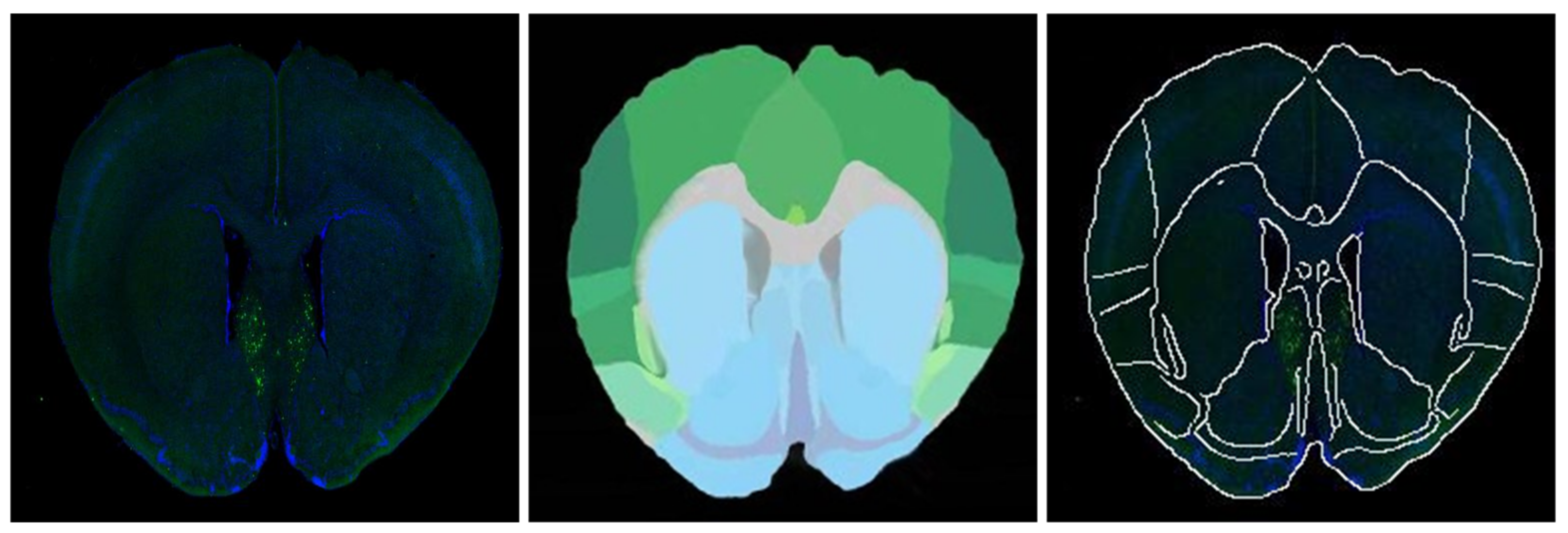
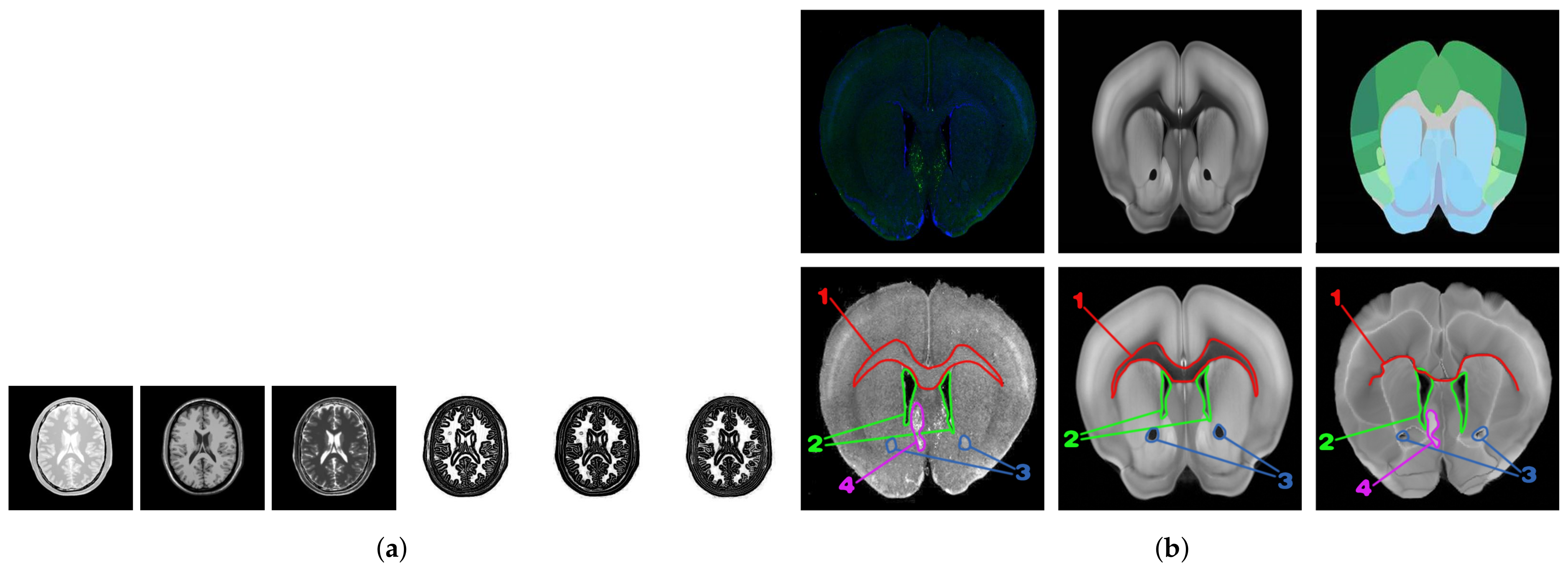
Most of the above modal transformation methods based on image representation are tested with T1-weighted, T2-weighted, and PD-weighted MR image data sets as the standard. Although the MR image data set is an image in three different modalities, its key features have a relatively simple correspondence and minimal noise interference. The modal transformation result of the ZMLD method with better performance is shown in Figure 1a. It can be seen from the figure that the modal transformation method can accurately extract the features of the three MR images and represent them to a unified modal. For the mouse brain slices (upper, left), namely the ATA (upper, middle) and ADA (upper, right) employed in this study, the specific morphological features are shown in the first row of Figure 1b, and there was a great difference in the corresponding key features between the original brain slices and the two kinds of the ARA. After the grayscale and affine transformation image preprocessing, the modalities between the grayscale brain slice (bottom, left) and ATA (bottom, middle) were closer, and they were selected for registration to use our approach without any processing. The results are shown in the second row and the three columns of Figure 1b. Regions 1, 2, and 3 in the brain slice images correspond to the ATA images, but the corresponding relationship of color features was very complex. Because of the inconsistency of this corresponding relationship and the difficulty of identifying boundary information, there is no unified standard for algorithm learning. Using the two non-unified modal images for training, the error correspondence was established, as shown in the second line (right) of Figure 1b. Moreover, the registration results were seriously affected by noise interference in the labeled region 4 in the brain slice. Owing to the differences in non-unified modality, more complex feature correspondence, and noise interference between the brain slice and ATA, conventional direct multi-modal image registration algorithms and existing image registration algorithms based on modal transformation made it difficult to realize the ideal regional localization.

Inspired by the fact that human experts automatically ignore the influence of noise when dealing with the regional localization of brain slices, the regional localization of each characteristic part on the brain slices is carried out by referring to the ARA. We proposed a novel idea of building correspondence based on key features. The corresponding key feature maps can be extracted from the brain slice and the ARA at the same time, and they can be converted into unified modal images. Then, the modal transformation problem can be transformed into an image segmentation problem. Since Long [18] and others first used Fully Convolutional Networks (FCNs) for end-to-end segmentation of natural images, image segmentation has made a breakthrough. SegNet [19], U-Net [20], and FC-DenseNet [21] have been proposed, although subsequent methods have achieved better segmentation results, and these methods are based on encoder–decoder network architecture. Given the satisfactory results achieved by the encoder–decoder architecture in the field of image segmentation, we proposed a new deep learning network architecture JEMI, and through the joint enhancement of multi-modal information, the modal transformation of brain slice and the ARA was effectively realized. Furthermore, the effect of image registration was improved by combining the diffeomorphic registration network based on unsupervised learning. Finally, with reference to the ARA, the automatic regional localization of brain slice images was completed. The brain slice image region localization framework proposed in this study is shown in Figure 2, but this method can be extended to any non-unified multi-modal image registration task.

2. Background

2.1. Mouse Brain Slice Image Acquisition

The mouse brain slice image acquisition was mainly divided into three steps: Neurotropic virus injection, sampling and sample preparation, and immunohistochemistry and confocal imaging. First, 8-week-old adult mice were prepared for disinfection and anesthesia, and then the target areas of their brains were injected with Japanese Encephalitis Virus (JEV) [22], which can express fluorescent proteins. After the virus was expressed in the mouse brain for 7.5 days, the mouse was over-anesthetized, and then cardiac perfusion was performed. The brain tissue of the mouse was taken out, soaked in paraformaldehyde fixative solution overnight, sliced with a shaking microtome, and then placed in a 24-well plate containing phosphate buffer for preservation. Finally, the target sections were immunohistochemically treated with 10% sheep serum and anti-JEV virus. Finally, the 10% sheep serum was used for immunohistochemical processing, and blue-green-red trichromatic channel fluorescence imaging of the brain slices was performed by a confocal microscope (LeicaSP8) to derive the Tiff format images.

2.2. Image Registration

The ultimate purpose of image registration is to establish the corresponding relationship between two images and to determine the geometric transformation relationship between them to correct the deformation of the image. In general, the invariant one of the two images is called the reference image (Fixed image), represented by F, and the changed one is called the floating image (Moving image), represented by M. Here, $F\left(x,y\right)$ and $M\left(x,y\right)$ denote the gray value of the reference image and the floating image at point $\left(x,y\right)$. The mathematical relationship between the reference image F and the floating image M can be expressed as:

$$F\left(x,y\right)=M\left(f(x,y)\right)$$

(1)

where f represents the two-dimensional geometric transformation function. For non-rigid registration, the transformation function of each point in the image is not necessarily the same. If the transformation parameters of each point are converted into displacement vectors, the displacement vector of the whole image forms a spatial deformation field, which is represented by $\varphi$. The main task of registration is to find $\varphi$ to make the deformed floating image, $\varphi$, and the reference image, F, as similar as possible.

2.3. Diffeomorphism

To ensure that the spatial deformation field is smooth and reversible, the inverse mapping is smooth, and the topological structure of the image does not change, the concept of diffeomorphic space was proposed in [23]. The diffeomorphic space is a Lie Group, which is a special manifold, and the group operation is smooth. There is a one-to-one mapping relationship between the Lie Group and Lie algebra, and the Lie algebra (g) is mapped to the Lie Group (G) space by exponential mapping. The deformation field is defined through the following ordinary differential equation (ODE):

$$\frac{\partial {\varphi }^{\left(t\right)}}{\partial t}=v\left({\varphi }^{\left(t\right)}\right)$$

(2)

where ${\varphi }^{\left(0\right)}=Id$ is the identity transformation, and t is time. We integrated the stationary velocity field, v, over $t=\left[0,1\right]$ to obtain the final registration field, ${\varphi }^{\left(1\right)}$, and we found scaling and squaring [24] to be the most efficient. The integral of ODE represents a one-parameter subgroup of diffeomorphism. In group theory, ${\varphi }^{\left(1\right)}=exp\left(v\right)$, v is a member of Lie algebra, which is indexed to generate the element ${\varphi }^{\left(1\right)}$ of the Lie Group. From the properties of one-parameter subgroup, for any scalars t and $t^{\prime }$, $exp\left((t+t^{\prime })v\right)=exp\left(tv\right)\circ exp\left(t^{\prime }v\right)$, where ∘ is a composition map associated with the Lie Group. Starting from ${\varphi }^{(1/2^T)}=p+v\left(p\right)/2^T$, where p is a map of spatial locations, we use ${\varphi }^{(1/2^{t-1})}={\varphi }^{(1/2^t)}\circ {\varphi }^{(1/2^t)}$ in a loop to obtain ${\varphi }^{\left(1\right)}={\varphi }^{\left(1/2\right)}\circ {\varphi }^{\left(1/2\right)}$ and select T to minimize $v/2^T$.

3. Methods

3.1. Rough Registration

Considering the individual differences among different animals and the large displacement caused by manual introduction when making brain slice images, it is difficult to establish a good corresponding relationship with the ARA. As such, rough registration is used for preliminary alignment of the brain slice and the ARA. After comparing the effects of each experimental method, the affine transformation model with more suitable performance was selected to make a preliminary rough registration of the mouse brain slice and the ARA to improve the effect of fine registration.

Affine transformation is a linear transformation from two-dimensional coordinates to two-dimensional coordinates, including translation, scaling, flipping, rotation, and shearing, which maintains the flatness and parallelism of the two-dimensional image. The transformation relationship can be expressed as follows:

$$\left\{\begin{array}{c}{x}^{\prime }=ax+by+m\hfill \\ y^{\prime }=cx+dy+n\hfill \end{array}\right.$$

(3)

It can also be expressed in the form of a matrix, as follows:

$$\left[\begin{array}{c}{x}^{\prime }\hfill \\ y^{\prime }\hfill \end{array}\right]=\left[\begin{array}{c}\begin{array}{ccc}a& b& m\end{array}\hfill \\ \begin{array}{ccc}c& d& n\end{array}\hfill \end{array}\right]\left[\begin{array}{c}x\\ y\\ 1\end{array}\right]$$

(4)

where a, b, c, d, m, and n are model parameters. According to the deformation relationship between the brain slice and the ARA, affine transformation with simple parameters and fast operation is the best transformation model we obtained by extracting the gray features of mouse brain slices and corresponding the ATA. Then, the model parameters of affine transformation are fitted by the nonlinear-least-square method to make the features of the two images correspond roughly. Finally, bilinear interpolation is carried out for the transformed images to preserve higher accuracy. By observing the effect of each fusion image, it was found that the characteristics of brain slices and the ARA after affine transformation were roughly aligned, and the effect was the best.

3.2. Modal Transformation

3.2.1. Model Building

Because of the differences in modal characteristics between the brain slice and the ARA, it is difficult for conventional direct image registration algorithms to establish a unified standard for learning, and the modal transformation method based on image representation cannot accurately represent different information. Inspired by human experts’ methods, that is, ignoring noise interference and establishing a corresponding relationship based on key regions when dealing with such problems, this study proposed converting the modal transformation task into an image segmentation task and realizes modal transformation by segmenting the corresponding features on the brain slice and the ARA. At present, the symmetric encoder–decoder network has become a classical framework in the field of image segmentation, and most of the latest proposed networks are modified based on it [25,26,27]. In this network architecture, the encoder uses the convolution network to extract image features with different depths, and the abstraction of features increases with increasing feature depth. The decoder uses the deconvolution operation to gradually transform the advanced features extracted by the encoder into classified pixel features, but image segmentation requires the classification ability of the network with pixel-level features. It is also necessary to project the features extracted by the encoder at different stages to the corresponding spatial position. The use of the jump connection mechanism solves this problem well, and more accurate segmentation results can be generated by combining deep and abstract high-level feature information with shallow and fine low-level feature information.

Given the good effect of the symmetric encoder–decoder network in the field of image segmentation, first, the U-Net network, which is suitable for small amounts of sample data and can enhance the data, is used to extract the features of brain slices and the ATA. For the ATA with obvious features, the U-Net network could accurately identify the feature shape and extract it for modal transformation, but, for brain slices with a lot of noise and inconspicuous key features, the performance of the U-Net network was not satisfactory. Considering that modal transformation aims to extract common corresponding features of multi-modal images and transform them into monomodal image features, an image segmentation network based on Joint Enhancement of Multimodal Information (JEMI) was proposed. It imitates the network architecture of the classical symmetric encoder–decoder and jump connection mechanism for multi-modal feature extraction and modal transformation of the brain slice and the ATA. Unlike other networks, this network trains the information of brain slices and the ATA together during input, hoping that the common feature information of different modal images can promote and restrict each other to obtain more accurate segmentation results and complete the modal transformation of the image.

3.2.2. Network Framework

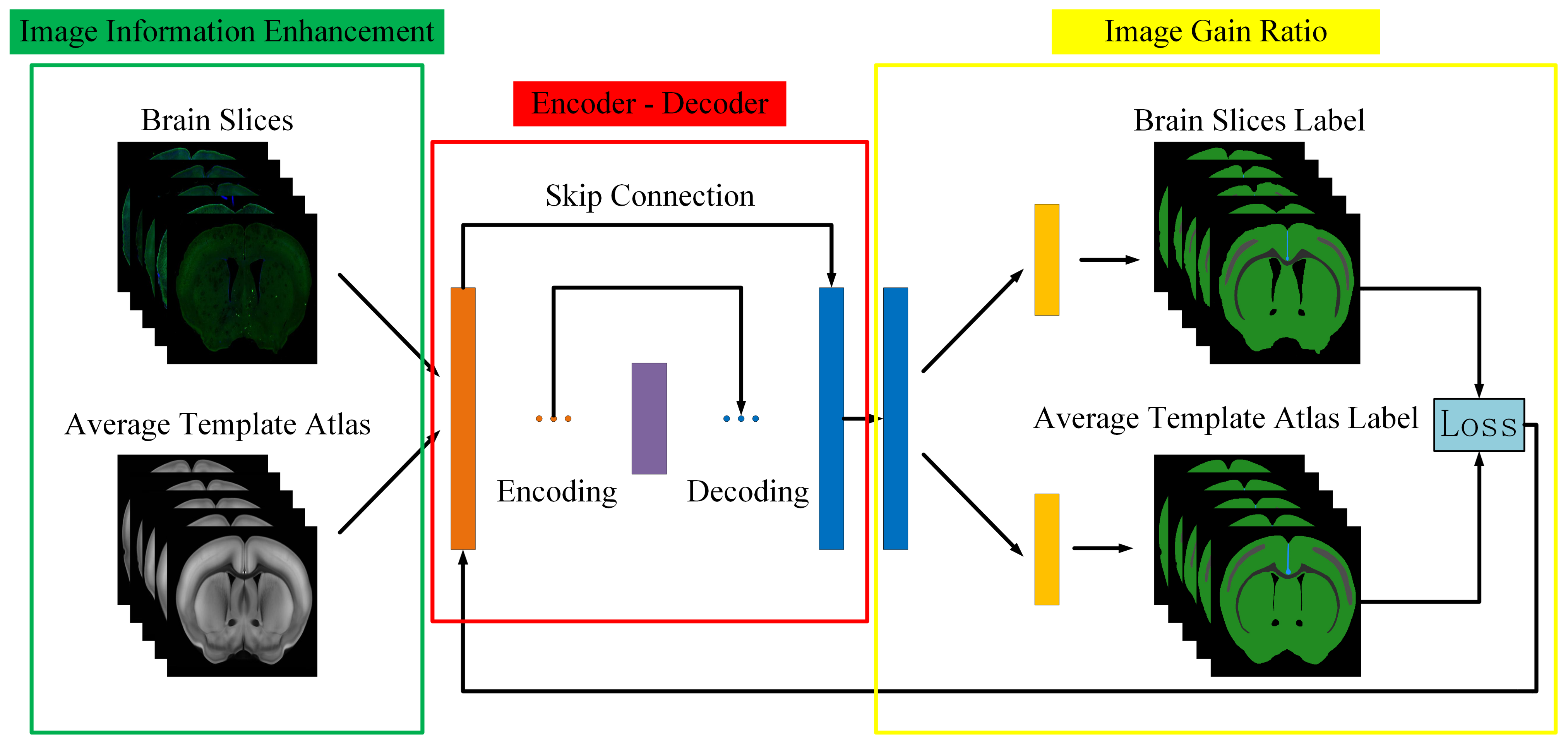
The JEMI network consists of three parts: image information enhancement, the symmetric encoder–decoder, and the image-gain proportional coefficient. The network framework is shown in Figure 3. The information enhancement also includes two aspects: image information self-enhancement and image information joint enhancement. As the training set selects the representative brain slices of different depths of the mouse brain and the corresponding ATA to the label, the amount of data are less, so it is necessary to self-enhance the image information first to increase the anti-interference ability of the network model and the generalization ability of the data to prevent over-fitting. This is realized by using a 3 × 3 matrix for random rotation, random translation, random scaling, random shearing, and random flipping.

The joint enhancement of image information inputs the enhanced image information into the JEMI network and then superimposes the information for the two non-unified modal images before training. When the symmetric encoder–decoder performs feature extraction on the combined information, the network can make full use of the consistency of image key structural features and context information, promote and constrain each other, and make reasonable mapping of the learned features to complete the modal transformation. The JEMI network has two inputs of the same size, and its dimensions are $B\times H\times W\times C$, where B is the size of the input batch, $H\times W$ is the size of the input image, and C is the number of channels of the input image. This study used fluorescent labeled brain slices derived by confocal microscopy and the ATA images for modal transformation, so C is equal to 3 at the input stage, and the size of the combined image information is $B\times H\times W\times 2C$.

In the symmetric encoder–decoder part, we first encode the multi-modal joint information, downsampled. Referring to the theory of Karen Simonyan [28], the convolution kernel of 3 × 3 size is used to extract features, which reduces the parameters and increases the nonlinearity at the same time. In the convolution operation of an image, each convolutional layer convolves the image matrix output from the previous layer with multiple convolution cores, followed by an additive bias. After the activation of the Rectified Liner Unit (ReLU), the new value is output to increase the nonlinear performance of the network, thus forming a new feature image. The padding in the convolution layer uses the ‘same’ to ensure that the decoded image is the same size as the original input image. The output of each neuron in the convolution layer is:

$$Y_j^L=f\left(\sum _{i=1}^{N^{L-1}}{Y}_i^{L-1}\otimes w_{ij}^L+b_j^L\right)$$

(5)

where $L-1$ and L are expressed as the layer depth of the network, $f\left(·\right)$ is expressed as an activation function, ⊗ represents a convolution operation, $Y_j^L$ is represented as the characteristic image of the j output of the L layer, $Y_i^{L-1}$ is represented as the characteristic image output by the $L-1$ layer. $w_{ij}^L$ and $b_j^L$ represent the multiplicative and additive paranoia of the L layer, respectively. The pooling layer is used between the convolutional layers to perform feature selection and information filtering on the output feature map, compress the amount of data and parameters, reduce the degree of overfitting, and complete the downsampling of the image. After four-layer convolution, the encoder downsamples the feature information after each layer convolution to obtain the multi-level high-dimensional features of the image and then decodes the high-dimensional features obtained by coding, that is, upsampling. In fact, upsampling realizes the mapping operation of an image from small resolution to large resolution. There are three common methods: bilinear, deconvolution, and unpooling. In this study, bilinear is used for upsampling, and then the upsampling image features are convoluted to complete the decoding operation. It should be noted that the decoded high-resolution image output information of each layer should be combined with the corresponding output information of the coding network to obtain more accurate pixel classification and spatial location.

As for image gain ratio, the features of the ATA image are more obvious than brain slice images, and it is easier to extract in the same U-net network, so a different convolution was carried out after the final output of the symmetric encoder–decoder to generate the prediction results of two different images. The prediction results are compared with their respective artificial feature labels, and binary cross entropy is used as the loss function to iteratively optimize the prediction results, the influence of different weights on the modal conversion results is tested, and the most appropriate weight parameters are selected for saving. The new brain slices and the ATA images are sent to the JEMI network loaded with the weights after training, which can directly extract the corresponding features of different modal brain images and complete the transformation from a multi-modal image to a monomodal image.

3.3. Fine Registration

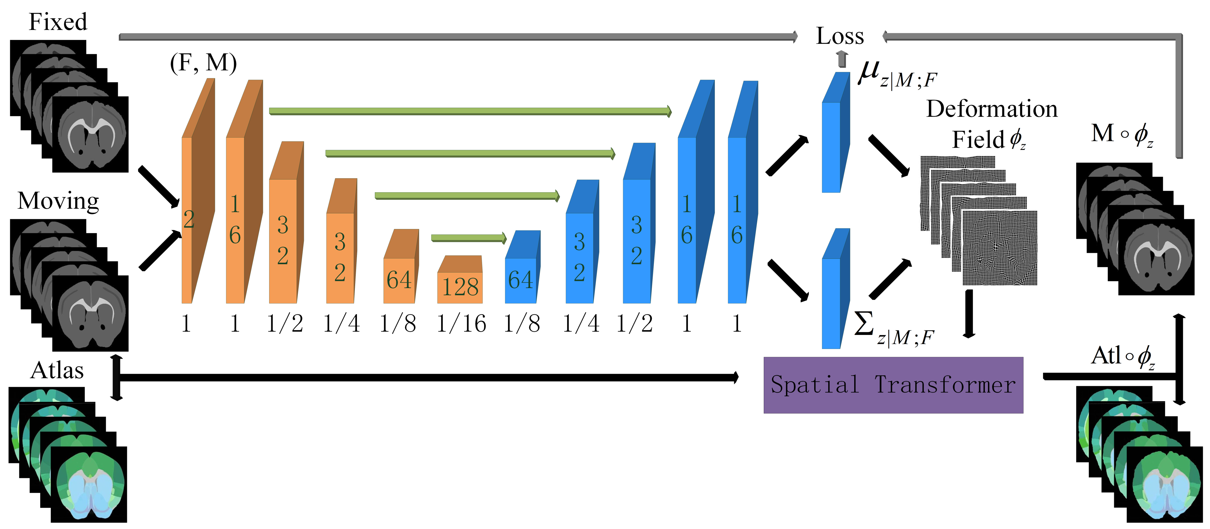
After the rough registration of affine transformation, a rough correspondence was established between the features of brain slices and the ARA images, but there were still many mismatched features. To keep the topological structure of the image unchanged during the deformation, a non-rigid registration network with diffeomorphic was introduced to deform the ARA. This method uses the convolutional neural network, diffeomorphic mapping, and a spatial transformation layer [29], and performs fast non-rigid registration of images in an unsupervised manner. Its network framework is shown in Figure 4.

3.3.1. The Construction of the Objective Function

Using z as a variable parameter of the spatial deformation field, $\varphi$, the model derivation [30] introduces the process of distorting M into F through $M\circ {\varphi }_z$. Modeling the prior probability of the parametrization z was done as follows:

$$p\left(z\right)=N(z;0,{\Sigma }_z)$$

(6)

where $N(·;\mu ,\Sigma )$ is the multivariate normal distribution with the mean $\mu$ and covariance $\Sigma$, and z is a stationary velocity field that specifies a diffeomorphism through the ODE. Moreover, $L=D-A$ is the Laplacian of a neighborhood graph defined on the voxel grid, where D is the graph degree matrix, and A is a voxel neighborhood adjacency matrix. We set ${\Sigma }_z^{-1}={\Lambda }_z=\mathsf{\lambda }L$ to realize the spatial smoothness of the velocity field z, where ${\Lambda }_z$ is a precision matrix and $\mathsf{\lambda }$ denotes a parameter controlling the scale of the velocity field z.

Moreover, F is a noisy observation of warped image M:

$$p\left(F\left|z;M\right.\right)=N(F;M\circ {\varphi }_z,{\sigma }_{}^2)$$

(7)

where ${\sigma }^2$ captures the variance of additive image noise.

We aim to estimate the posterior registration probability $p\left(z\right|F;M)$. Using this, we can obtain the most likely registration field ${\varphi }_z$ for a new image pair $(F,M)$.

Because the calculation of posterior probability $p\left(z\right|F;M)$ is more difficult, we take a variational approach. By introducing an approximate posterior probability $q_{\psi }\left(z\right|F;M)$ parametrized by $\psi$, we minimize the $KL$ divergence:

$$\begin{array}{c}\underset{\psi }{min}KL[q_{\psi }\left(z\right|F;M)\left|\right|p\left(z\right|F;M)]\hfill \\ =\underset{\psi }{min}KL[q_{\psi }\left(z\right|F;M)\left|\right|p\left(z\right)]-E_q[logp\left(F\right|z;M)]+const\hfill \end{array}$$

(8)

Modeling the approximate posterior $q_{\psi }\left(z\right|F;M)$ as a multivariate normal was done as follows:

$$q_{\psi }\left(z\right|F;M)=N(z;{\mu }_{z|M;F},{\Sigma }_{z|M;F})$$

(9)

where ${\Sigma }_{z|M;F}$ is diagonal, and the statistics ${\mu }_{z|M;F}$ and the diagonal of ${\Sigma }_{z|M;F}$ can be interpreted as the voxel-wise mean and variance, respectively.

We then estimate ${\mu }_{z|M;F}$ and ${\Sigma }_{z|M;F}$ using a convolutional neural network parameterized by $\psi$. Based on $KL$ divergence using the stochastic gradient method, we can optimize by $\psi$ parameterized approximate posterior probability $q_{\psi }\left(z\right|F;M)$. Specifically, for each image pair $(F,M)$ and sample $z_k\sim q_{\psi }\left(z\right|F;M)$, we can calculate $M\circ {\varphi }_{z_k}$, with the resulting loss as follows:

$$\begin{array}{c}L(\psi ;F,M)=KL[q_{\psi }\left(z\right|F;M)\left|\right|p\left(z\right)]-E_q[logp\left(F\right|z;M)]\hfill \\ =\frac{1}{2}[tr(\mathsf{\lambda }D{\Sigma }_{z|M;F}-log{\Sigma }_{z|M;F})+{\mu }_{{}_{z|M;F}}^T{\Lambda }_z{\mu }_{z|M;F}]\hfill \\ +\frac{1}{2{\sigma }^{2}K}{\displaystyle \sum _k}{∥F-M\circ {\varphi }_{z_k}∥}^2+const\hfill \end{array}$$

(10)

where K is the number of samples used to approximate the expectation. The first term brings the approximate posterior probability closer to the prior probability. The variational covariance ${\Sigma }_{z|M;F}$ is diagonal, and the last term spatially smoothens the mean, which can be seen by expanding ${\mu }_{{}_{z|M;F}}^T{\Lambda }_z{\mu }_{z|M;F}=\frac{\mathsf{\lambda }}{2}\sum {\sum }_{j\in N\left(I\right)}{(\mu \left[i\right]-\mu \left[j\right])}^2$, where $N\left(I\right)$ are the neighbors of voxel i. The second term makes the distorted image $M\circ {\varphi }_{z_k}$ more similar to the reference image F, and ${\sigma }^2$ and $\mathsf{\lambda }$ represent fixed hyper-parameters.

3.3.2. Fine Registration Network Framework

We designed an architecture based on U-net with F and M as input, and the feature parameter extraction network contains the mean parameter ${\mu }_{z|M;F}$ and covariance ${\Sigma }_{z|M;F}$ as output, as shown in Figure 4. The network has symmetrical downsampled and upsampled architecture, and after upsampling, it is connected to the corresponding downsampled part to get more detailed features. All convolutional layers use 3 × 3 kernels and LeakyReLu activations.

In general, the neural network takes the reference image F and floating image M as inputs to calculate the mean parameter, ${\mu }_{z|M;F}$, and the covariance, ${\Sigma }_{z|M;F}$, and uses a re-parameterization trick to sample the new velocity field $z_k\sim N({\mu }_{z|M;F},{\Sigma }_{z|M;F})$. According to $z_k$, ${\varphi }_{z_k}$ with diffeomorphism is calculated and the floating image M is transformed spatially. Each of the above steps is designed to be differentiable, so a method based on stochastic gradient descent can be used, according to the $Loss$ function $L(\psi ;F,M)$, to continuously learn and optimize the network parameters, and finally realize the fine registration of brain slice images.

3.4. Performance Evaluation

After the optimal spatial deformation field is obtained, the spatial transformation layer can be used to apply the spatial deformation field to the ADA to evaluate the performance of the registration results. The ADA has rich regional division information, and different brain regions are separated by different colors. Thus, the edges of regions can be easily extracted, and then the edges of the regions are fused with the brain slices to complete the localization of the regions in the mouse brain slices. The performance of different methods was compared with the accuracy of localization, and the results are shown in Figure 5.

4. Experiments and Result Analysis

4.1. Software and Hardware Environment

Software environment: The experiment was built on the PyCharm platform, and the implementation of the Keras deep learning framework was based on Tensorflow. The language version used was Python 3.6.4.

Hardware environment: The experiment was run on the Windows 10 operating system. The CPU was Intel Core-i7 (3.20 GHz), the memory was 64 GB, the graphics card was NVIDIA GeForce GTX 1080Ti, and the video memory was 11 GB.

4.2. Data Set Production and Training

In the experiment, immunohistochemical brain slices of a mouse with confocal microscopy imaging and the second edition of the ARA were used to establish data sets. First, a group of mouse brain slices was selected, and then the ADA and ATA of the corresponding mouse brain slices were found in the ARA data set, and the brain slice images were pre-processed (through denoising, for example) and adjusted to the same size as the ARA. As the image was still too large for the algorithm to run, all three images were compressed to a smaller size (512 × 512) of the same size for fast processing. Then, the grayscale features of ATA, which were more similar to brain slices, were extracted and roughly registered by affine transformation so that the morphological features of the ATA were closer to brain slices. Finally, the brain slice and Brain Atlas were sent to the JEMI network for modal transformation. The key feature segmentation data sets of the brain slice, $F^{\prime }$, and the ATA, $M^{\prime }$, were then generated and sent to the fine registration network for training to obtain the optimal deformation field. A total of 64 groups of images were used for training, 18 groups of images were used for verification, and 18 groups of images were used for testing.

4.3. Experimental Results and Analysis

To verify the effectiveness of the method proposed in this article, some comparative experiments were carried out for each step, and the performance of each method was evaluated from different aspects. In the rough registration stage, the Run Time (RT), Normalized Correlation Coefficient (NCC), and Normalized Mutual Information (NMI) were used to evaluate the performance of different methods. The strategy was calculated according to (11) and (12):

$$NCC\left(I,J\right)=\sum _{p\in \Omega }\frac{{\sum }_p\left(I\left(p\right)-\widehat{I}\left(p\right)\right)\left(J\left(p\right)-\widehat{J}\left(p\right)\right)}{\sqrt{{\sum }_p{\left(I\left(p\right)-\widehat{I}\left(p\right)\right)}^2{\sum }_p{\left(J\left(p\right)-\widehat{J}\left(p\right)\right)}^2}}$$

(11)

where I and J represent two images, and p represents the pixels in the two images. NCC is one of the most widely used image similarity measures, which can reflect the degree of image correlation. Its value range was between [−1, 1]. The closer the correlation coefficient to 1, the more similar the two images.

$$NMI\left(I,J\right)=\frac{H\left(I\right)+H\left(J\right)}{H\left(I,J\right)}$$

(12)

where $H\left(I\right)$ is the information entropy of the image, and its calculation formula is $H\left(I\right)=-{\displaystyle \sum _{i=0}^{N-1}}{p}_{i}log{p}_i$; $p_i$ is the probability of gray value i, calculated according to the formula $p_i=h_i/\left({\displaystyle \sum _{i=1}^{N-1}}{h}_i\right)$; $h_i$ represents the total number of pixels with the gray value i in the image; and N represents the number of gray levels of the image. Moreover, $H\left(I,J\right)$ is the joint information entropy of the two images, and the calculation formula is $H\left(I,J\right)=-{\displaystyle \sum _{i,j}}{p}_{IJ}\left(i,j\right)log{p}_{IJ}\left(i,j\right)$. NMI is currently one of the indicators commonly used in image registration, which can indicate the degree of mutual inclusion of two image information. The larger the normalized mutual information, the better the registration effect between the two images.

In the modal conversion stage, the Pixel Accuracy (PA), the Mean Pixel Accuracy (MPA), the Mean Intersection over Union (MIoU), and the Frequency Weighted Intersection over Union (FWIoU) were used to evaluate the performance of different methods. The evaluation strategy was calculated according to (13)–(16):

$$PA=\frac{{\sum }_{i=0}^k{p}_{ii}}{{\sum }_{i=0}^k{\sum }_{j=0}^k{p}_{ij}}$$

(13)

$$MPA=\frac{1}{k+1}\sum _{i=0}^k\frac{p_{ii}}{{\sum }_{j=0}^k{p}_{ij}}$$

(14)

$$MIoU=\frac{1}{k+1}\sum _{i=0}^k\frac{p_{ii}}{{\sum }_{j=0}^k{p}_{ij}+{\sum }_{j=0}^k{p}_{ji}-p_{ii}}$$

(15)

$$FWIoU=\frac{1}{{\sum }_{i=0}^k{\sum }_{j=0}^k{p}_{ij}}\sum _{i=0}^k\frac{p_{ii}}{{\sum }_{j=0}^k{p}_{ij}+{\sum }_{j=0}^k{p}_{ji}-p_{ii}}$$

(16)

We supposed there were $K+1$ classes, including a background class, where $p_{ii}$ represents the number of pixels predicted correctly for all classes, $p_{ij}$ represents the number of pixels that belong to class i but are predicted to be class j, and $p_{ij}$ and $p_{ji}$ are called false positives and false negatives, respectively. PA is the ratio of correctly marked pixels to the total pixels. MPA calculates the ratio of correctly classified pixels in each class and then calculates the average of all classes. MIoU is a standard metric for semantic segmentation, which calculates the sum of the intersection of the true value and the predicted value. FWIoU is an improvement of MIoU, and weights were set for each class according to the frequency of appearance to judge the accuracy of the prediction.

In the fine registration stage, image fusion and the aforementioned RT, NCC and NMI were used for performance evaluation.

4.3.1. Rough Registration

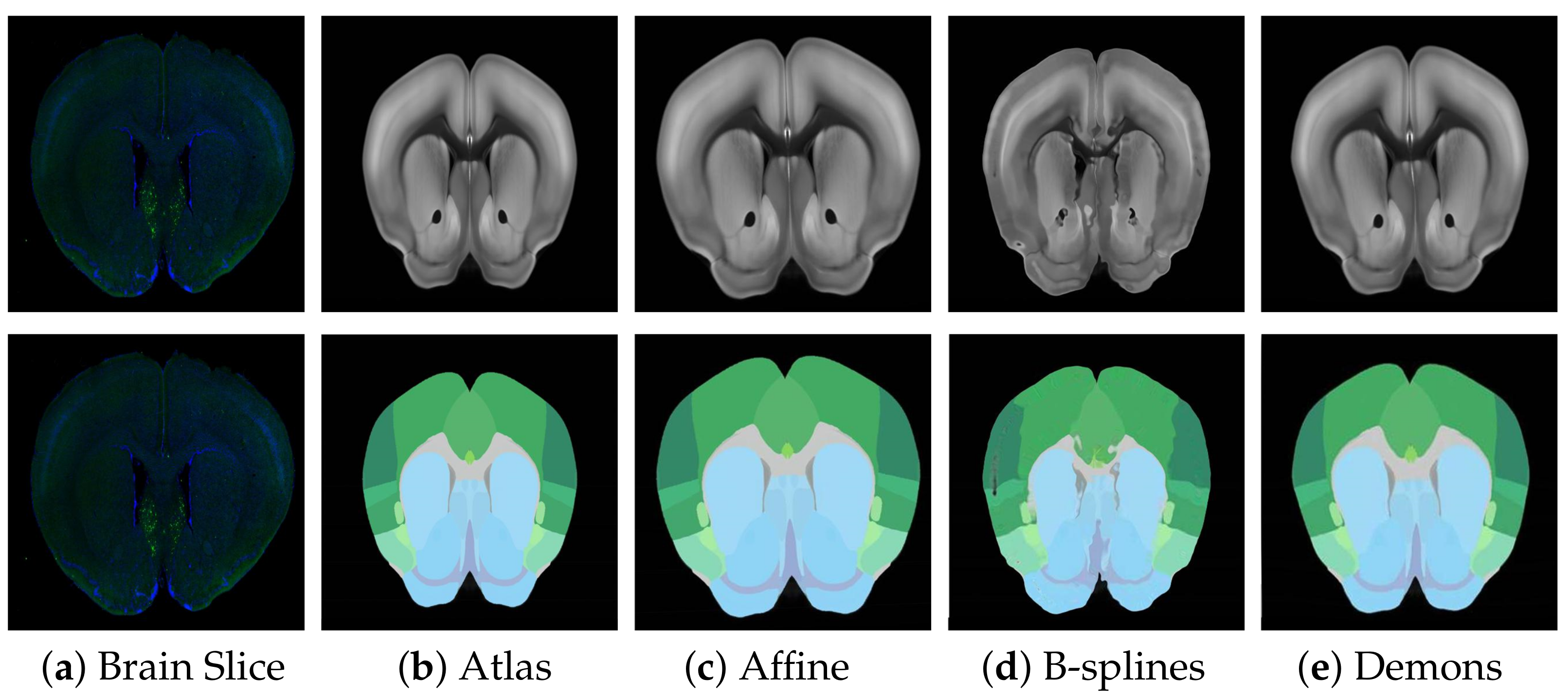
Before fine registration, preliminary rough registration of brain slices and standard brain atlas can effectively reduce the difficulty of registration and improve the effect of fine registration. Therefore, choosing a suitable rough registration method is vital. In this study, affine transform, traditional B-splines [31], and Demons [32] were selected for testing, and the experimental results are shown in Figure 6. The performance comparison results using RT, NCC, and NMI measurement strategies are shown in

Table 1. Comparison of the results of different methods of rough registration.

Method	CPU RT sec	NCC	NMI
Original image pairs	-	0.586757	1.068795
B-splines	413	0.719663	1.085182
Demons	237	0.733310	1.089640
Affine	219	0.804499	1.097789

. Obviously, affine transformation was the most suitable rough registration method because of its faster speed and better effect.

4.3.2. Modal Transformation

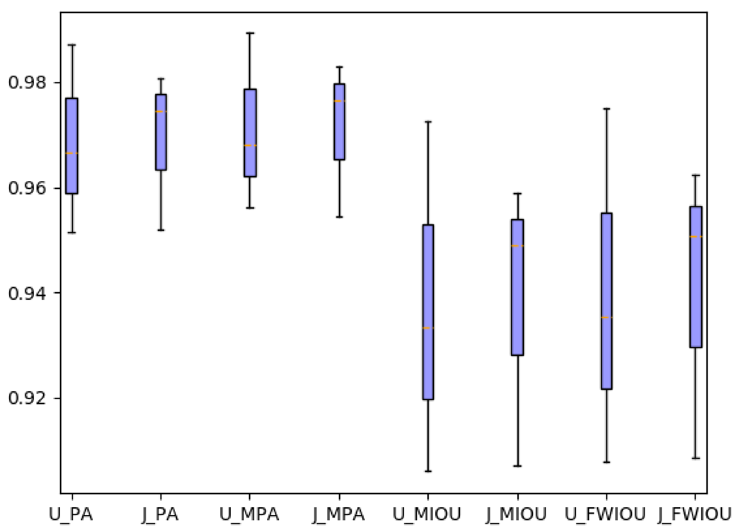
To better solve the problem of non-unified multi-modal image registration, using the modal transformation method to convert a multi-modal image into a monomodal image is an effective method. In this study, a Joint Enhancement of Multimodal Information image segmentation method was proposed. It segments the corresponding key features in the image to complete the modal transformation. To verify the performance of the proposed method, the U-Net network suitable for small samples was selected for comparison, and the results are shown in Figure 7. The commonly used evaluation indicators of PA, MPA, MIOU and FWIOU for image segmentation were used. The results were evaluated, and the performance analysis is shown in Figure 8.

The experimental results indicate that the U-Net network can accurately segment the ATA images with obvious features and less noise. As for some brain slice images with no obvious features and a lot of noise, they could not recognize the key features or achieve satisfactory segmentation results. The JEMI network proposed in this study trains two multi-modal images together, and, by fusing the input multi-modal information, it can both promote and enhance the learning of key features and also restrict the influence of marker neurons to achieve a better effect of modal transformation ultimately.

4.3.3. Fine Registration

To verify the performance of the modal transformation method proposed in this study and the performance of the diffeomorphic registration method, three comparative experiments were carried out.

(1)

Modal transformation effects

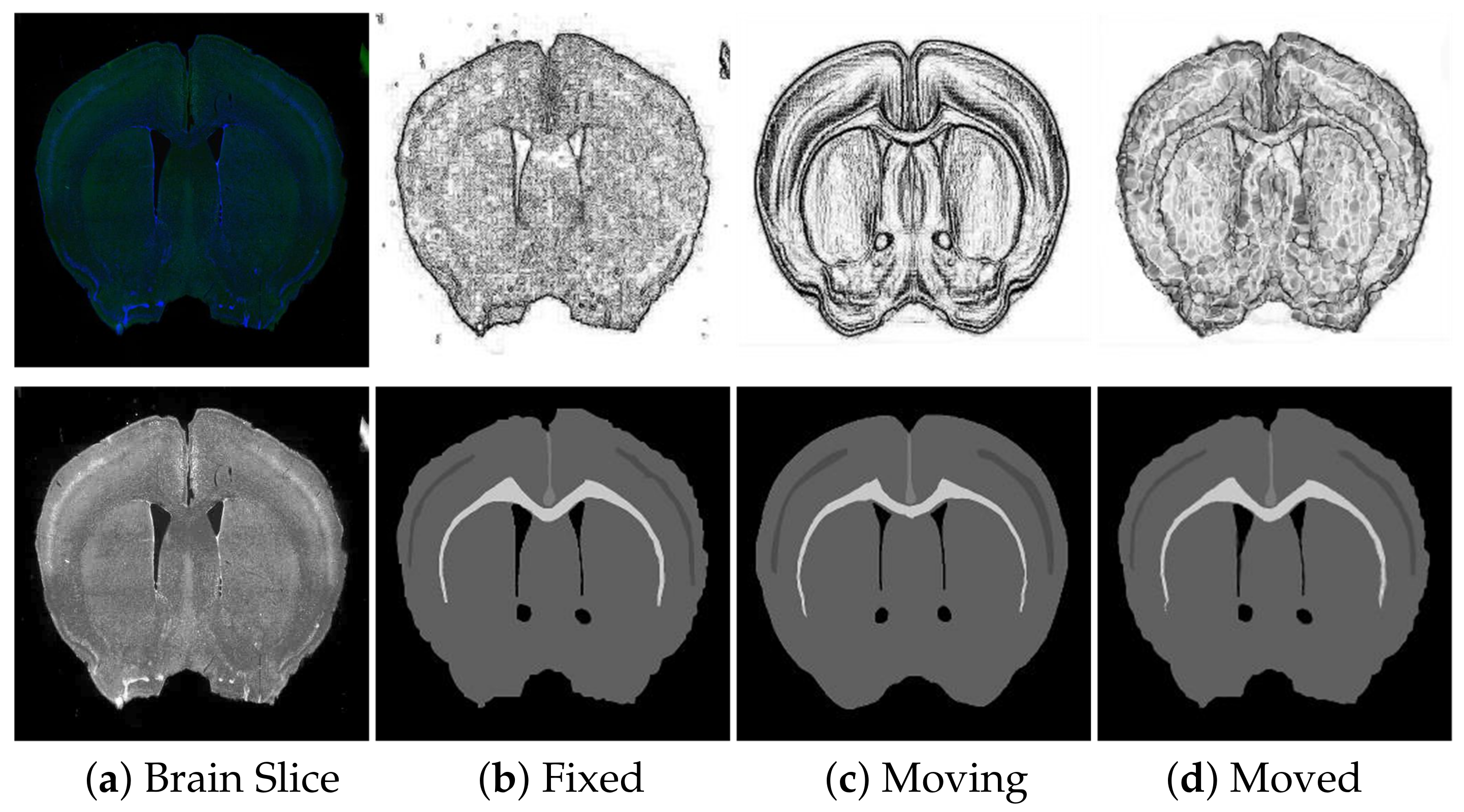
To verify the impact of modal transformation on registration results, the data set was registered once in the absence of modal transformation and then again with the same registration method with other parameters unchanged. The experimental registration results are shown in Figure 9.

The experimental results indicate that modal transformation plays an important role in the registration results. Without modal transformation, the corresponding features between the brain slices and Brain Atlas were both of the mutual reference and non-reference types. Some were easy to identify, and some were difficult to distinguish from the surrounding environment, and there might be noises such as labeled neurons and staining on the brain slices. The registration results are shown in Figure 9c. The registration algorithm could not accurately identify the complex corresponding relationship between brain slices and the Brain Atlas, pull and deform the internal features, or retain the topological structure of the original image. The image noise also interfered with the results. After the modal transformation, the registration algorithm could effectively deform the Brain Atlas Image features and align with the brain slice, overcoming the complex feature correspondence and image noise, and achieving a better registration effect.

(2)

Different modal transformation methods

To further verify the superiority of the JEMI method, we compared the PCA modal transformation method with the JEMI modal transformation method. The PCA modal transformation method re-characterizes the extracted feature information by extracting multi-level features of the image and performing feature fusion, which can convert images of different modalities into similar modalities, reducing the difference between modalities. Two different modal transformation images were sent into the registration network for registration, and the results are shown in Figure 10.

The experimental results indicate that different modal transformation methods had a great influence on the registration results. Although the PCA modal transformation method represents the images of different modalities as new images with a similar modality, which reduced the effects of modal differences and labeled neuron noise, it also blurred many features, making it difficult to accurately identify feature location and causing a local blockage. It was better than the registration result without modal transformation, but it was still far from achieving the ideal effect. The JEMI method can completely transform the images of different modalities into a unified one, the feature correspondence is simple, and there is no noise interference. Thus, it could effectively identify the corresponding features and carry out the deformation with diffeomorphism. Without changing the topological structure of the image, the fine registration of brain slices and the standard Brain Atlas was realized, and the regional localization could be completed accurately.

(3)

Different registration methods

To verify the superiority of the registration algorithm in this study, the traditional B-splines registration method, Demons registration method, and Reg-Net Registration method using Deep Learning were compared in the experiment. The fusion results of the brain slice and Brain Atlas after registration of each method are shown in Figure 11.

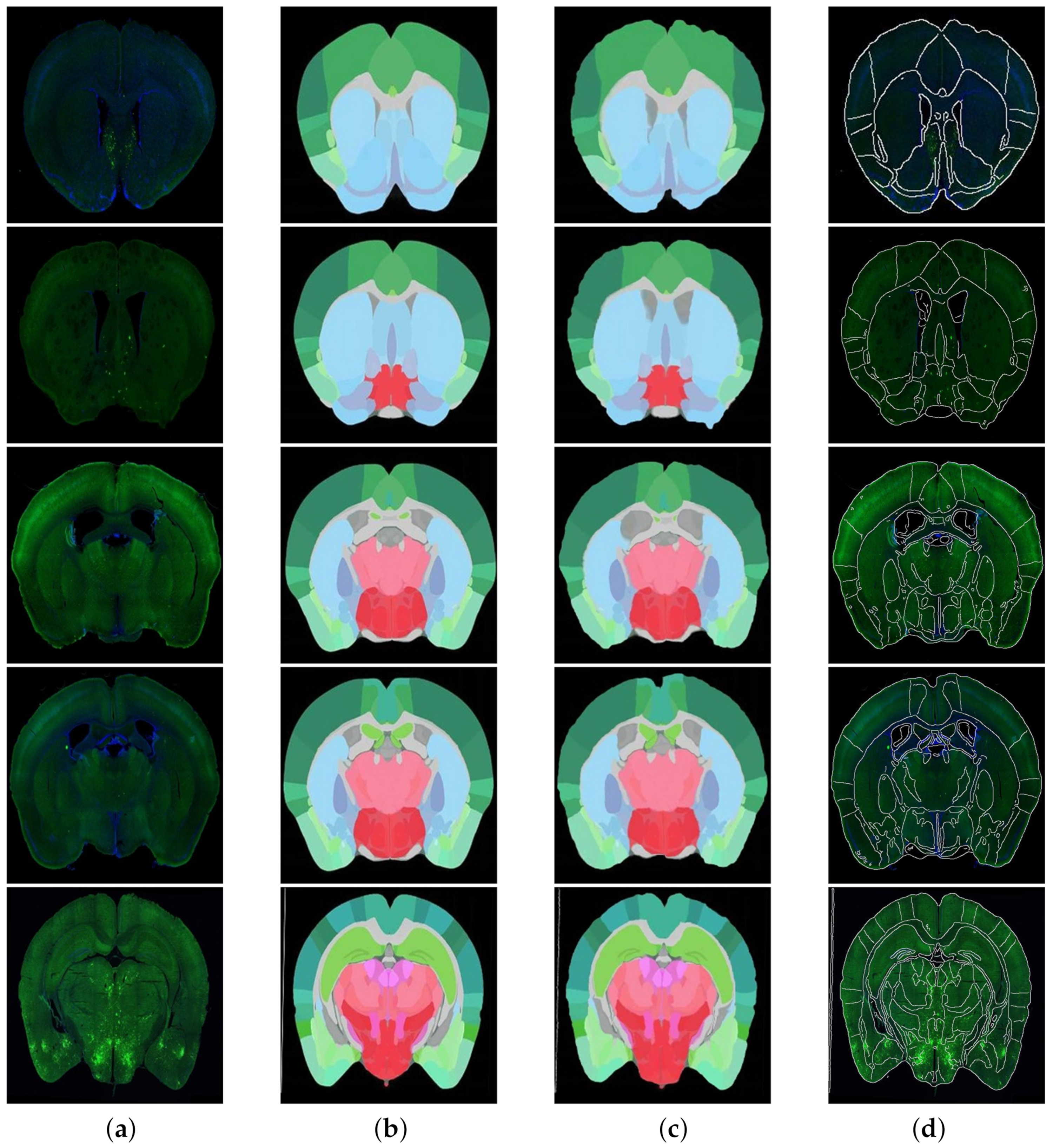
According to the fusion effect of images, the results of the regional localization method in this study were noticeably better than others. The external edge and internal feature contour fit well with the brain slice images, and the original topological structure was left unchanged. The regional localization effect of some brain slices is shown in Figure 12.

To quantify the performance of different methods, RT, NCC, and NMI were used to compare the brain slice and the deformed ATA. Using 18 groups of images, we carry out calculation of the above three indicators and compare them with average values, as shown in

Table 2. Quantitative evaluation of a registration model trained with different methods.

Method	CPU RT sec	NCC	NMI
Original image pairs	-	0.586757	1.068795
Affine + B-splines	567	0.843298	1.107714
Affine + Demons	426	0.823030	1.106063
PCA + Reg-Net	81	0.844939	1.111956
Ours	27	0.871956	1.113704

.

The experimental results indicate that the performance of the proposed method is better than that of existing methods. Compared with the PCA + REG-NET method, the RT of the registration results of this method was reduced by 66.66%, the NCC and NMI were increased by 3.20% and 0.16%, respectively, and excellent performance was achieved in each evaluation index. The experimental results indicate that this method can carry out unsupervised diffeomorphic registration for brain slice images with non-unified modality and can complete the localization of mouse brain slices accurately and quickly.

5. Conclusions

To solve the practical problem of brain slice regional localization in the mouse, the JEMI network for the unified modal transformation of multi-modal images was proposed in this study. It can be combined with the unsupervised diffeomorphic registration algorithm to achieve accurate and fast regional localization. We carried out experimental research on the modal transformation method and image registration method effects on the final effect, and the results indicate that, compared with the existing region location methods, this method has many advantages: simple operation, fast training, accurate results, the ability to overcome the influence of noise pollution and multi-modal images, and better performance in each index. This method can be used for regional localization of brain slice images on a large scale to carry out an in-depth analysis of experimental data on brain science research. It can also be extended to other multi-modal image registration tasks. In the future, we will study the method to extract smaller features of brain slices and promote the performance of registration.

References

1. Renier, N.; Adams, E.L.; Kirst, C.; Wu, Z.; Azevedo, R.; Kohl, J.; Autry, A.E.; Kadiri, L.; Venkataraju, K.U.; Zhou, Y.; et al. Mapping of brain activity by automated volume analysis of immediate early genes. Cell 2016, 165, 1789–1802. [Google Scholar] [CrossRef] [PubMed] [Green Version]
2. Jones, A.R.; Overly, C.C.; Sunkin, S.M. The Allen brain atlas: 5 years and beyond. Nat. Rev. Neurosci. 2009, 10, 821–828. [Google Scholar] [CrossRef]
3. Goldowitz, D. Allen Reference Atlas. A Digital Color Brain Atlas of the C57BL/6J Male Mouse-by HW Dong. Genes Brain Behav. 2010, 9, 128. [Google Scholar] [CrossRef]
4. Zitova, B.; Flusser, J. Image registration methods: A survey. Image Vis. Comput. 2003, 21, 977–1000. [Google Scholar] [CrossRef] [Green Version]
5. Haskins, G.; Kruger, U.; Yan, P. Deep learning in medical image registration: A survey. Mach. Vis. Appl. 2020, 31, 1–18. [Google Scholar] [CrossRef] [Green Version]
6. Leventon, M.E.; Grimson, W.E.L. Multi-modal volume registration using joint intensity distributions. In International Conference on Medical Image Computing and Computer-Assisted Intervention; Springer: Berlin/Heidelberg, Germany, 1998; pp. 1057–1066. [Google Scholar]
7. Maes, F.; Collignon, A.; Vandermeulen, D.; Marchal, G.; Suetens, P. Multimodality image registration by maximization of mutual information. IEEE Trans. Med. Imaging 1997, 16, 187–198. [Google Scholar] [CrossRef] [Green Version]
8. Wells, W.M., III; Viola, P.; Atsumi, H.; Nakajima, S.; Kikinis, R. Multi-modal volume registration by maximization of mutual information. Med. Image Anal. 1996, 1, 35–51. [Google Scholar] [CrossRef]
9. Viola, P.; Wells, W.M., III. Alignment by maximization of mutual information. Int. J. Comput. Vis. 1997, 24, 137–154. [Google Scholar] [CrossRef]
10. Roche, A.; Pennec, X.; Malandain, G.; Ayache, N. Rigid registration of 3D ultrasound with MR images: A new approach combining intensity and gradient information. IEEE Trans. Med. Imaging 2001, 20, 1038–1049. [Google Scholar] [CrossRef] [PubMed]
11. Wein, W.; Brunke, S.; Khamene, A.; Callstrom, M.R.; Navab, N. Automatic CT-ultrasound registration for diagnostic imaging and image-guided intervention. Med. Image Anal. 2008, 12, 577–585. [Google Scholar] [CrossRef]
12. Wachinger, C.; Navab, N. Entropy and Laplacian images: Structural representations for multi-modal registration. Med. Image Anal. 2012, 16, 1–17. [Google Scholar] [CrossRef] [PubMed]
13. Heinrich, M.P.; Jenkinson, M.; Bhushan, M.; Matin, T.; Gleeson, F.V.; Brady, M.; Schnabel, J.A. MIND: Modality independent neighbourhood descriptor for multi-modal deformable registration. Med. Image Anal. 2012, 16, 1423–1435. [Google Scholar] [CrossRef] [PubMed]
14. Yang, F.; Ding, M.; Zhang, X.; Wu, Y.; Hu, J. Two phase non-rigid multi-modal image registration using weber local descriptor-based similarity metrics and normalized mutual information. Sensors 2013, 13, 7599–7617. [Google Scholar] [CrossRef] [Green Version]
15. Chen, J.; Shan, S.; He, C.; Zhao, G.; Pietikäinen, M.; Chen, X.; Gao, W. WLD: A robust local image descriptor. IEEE Trans. Pattern Anal. Mach. Intell. 2009, 32, 1705–1720. [Google Scholar] [CrossRef]
16. Studholme, C.; Hill, D.L.; Hawkes, D.J. An overlap invariant entropy measure of 3D medical image alignment. Pattern Recognit. 1999, 32, 71–86. [Google Scholar] [CrossRef]
17. Zhu, X.; Ding, M.; Huang, T.; Jin, X.; Zhang, X. PCANet-based structural representation for nonrigid multimodal medical image registration. Sensors 2018, 18, 1477. [Google Scholar] [CrossRef] [PubMed] [Green Version]
18. Long, J.; Shelhamer, E.; Darrell, T. Fully convolutional networks for semantic segmentation. In Proceedings of the IEEE Conference on Computer Vision and Pattern Recognition, Boston, MA, USA, 7–12 June 2015; pp. 3431–3440. [Google Scholar]
19. Badrinarayanan, V.; Kendall, A.; Cipolla, R. Segnet: A deep convolutional encoder–decoder architecture for image segmentation. IEEE Trans. Pattern Anal. Mach. Intell. 2017, 39, 2481–2495. [Google Scholar] [CrossRef]
20. Ronneberger, O.; Fischer, P.; Brox, T. U-net: Convolutional networks for biomedical image segmentation. In International Conference on Medical Image Computing and Computer-Assisted Intervention; Springer: Berlin/Heidelberg, Germany, 2015; pp. 234–241. [Google Scholar]
21. Jégou, S.; Drozdzal, M.; Vazquez, D.; Romero, A.; Bengio, Y. The one hundred layers tiramisu: Fully convolutional densenets for semantic segmentation. In Proceedings of the IEEE Conference on Computer Vision and Pattern Recognition Workshops, Honolulu, HI, USA, 21–26 July 2017; pp. 11–19. [Google Scholar]
22. Jia, F.; Zhu, X.; Xu, F. A single adaptive point mutation in Japanese encephalitis virus capsid is sufficient to render the virus as a stable vector for gene delivery. Virology 2016, 490, 109–118. [Google Scholar] [CrossRef]
23. Ashburner, J. A fast diffeomorphic image registration algorithm. Neuroimage 2007, 38, 95–113. [Google Scholar] [CrossRef]
24. Arsigny, V.; Commowick, O.; Pennec, X.; Ayache, N. A log-euclidean framework for statistics on diffeomorphisms. In International Conference on Medical Image Computing and Computer-Assisted Intervention; Springer: Berlin/Heidelberg, Germany, 2006; pp. 924–931. [Google Scholar]
25. Ghosh, S.; Das, N.; Das, I.; Maulik, U. Understanding deep learning techniques for image segmentation. ACM Comput. Surv. (CSUR) 2019, 52, 1–35. [Google Scholar] [CrossRef] [Green Version]
26. Seo, H.; Badiei Khuzani, M.; Vasudevan, V.; Huang, C.; Ren, H.; Xiao, R.; Jia, X.; Xing, L. Machine learning techniques for biomedical image segmentation: An overview of technical aspects and introduction to state-of-art applications. Med. Phys. 2020, 47, e148–e167. [Google Scholar] [CrossRef]
27. Tajbakhsh, N.; Jeyaseelan, L.; Li, Q.; Chiang, J.N.; Wu, Z.; Ding, X. Embracing imperfect datasets: A review of deep learning solutions for medical image segmentation. Med. Image Anal. 2020, 63, 101693. [Google Scholar] [CrossRef] [PubMed] [Green Version]
28. Simonyan, K.; Zisserman, A. Very deep convolutional networks for large-scale image recognition. arXiv 2014, arXiv:1409.1556. [Google Scholar]
29. Jaderberg, M.; Simonyan, K.; Zisserman, A.; Kavukcuoglu, K. Spatial transformer networks. arXiv 2015, arXiv:1506.02025. [Google Scholar]
30. Dalca, A.V.; Balakrishnan, G.; Guttag, J.; Sabuncu, M.R. Unsupervised learning for fast probabilistic diffeomorphic registration. In International Conference on Medical Image Computing and Computer-Assisted Intervention; Springer: Berlin/Heidelberg, Germany, 2018; pp. 729–738. [Google Scholar]
31. Xie, Z.; Farin, G.E. Image registration using hierarchical B-splines. IEEE Trans. Vis. Comput. Graph. 2004, 10, 85–94. [Google Scholar]
32. Vercauteren, T.; Pennec, X.; Perchant, A.; Ayache, N. Diffeomorphic demons: Efficient non-parametric image registration. NeuroImage 2009, 45, S61–S72. [Google Scholar] [CrossRef] [PubMed] [Green Version]
Figure 1. (a) Multimodal MR images are often used in the study of modal transformation methods. The three on the left are T1-weighted, T2-weighted, and PD-weighted Magnetic Response Images; the three on the right are their result of modal transformation; (b) Display and registration of non-unified modal brain images. Top row: Brain Slice Image (left), ATA Image (middle), and ADA Image (right). Bottom row: The grayscale brain slice image (left, fixed) and the ATA image (middle, moving) were registered to generate the resulting image (right, moved). Among them, region 1 (red), region 2 (green), and region 3 (blue) represent corresponding features on different images, while region 4 (purple) represents neurons, which formed the image noise during the image registration process.
Symmetry 13 00929 g001
Figure 2. The whole framework of the regional localization method in the brain slice image.
Symmetry 13 00929 g002
Figure 3. Overview of the proposed Joint Enhancement of Multimodal Information Network architecture. It is divided into three parts: Image Information Enhancement, Encoder–Decoder, and Image Gain Ratio.
Symmetry 13 00929 g003
Figure 4. Illustration of our registration network architecture. The Grayscale brain slice and ATA take two characteristic parameters of the mean and covariance after the convolution neural network and then use the re-parameterization technique and integral to obtain the deformation field. Finally, spatial transformation is implemented for the ADA to complete registration.
Symmetry 13 00929 g004
Figure 5. Regional localization result after image fusion.
Symmetry 13 00929 g005
Figure 6. Examples across different transformation methods on the Atlas dataset. Top: Brain Slice image, ATA with different deformations. Bottom: Brain Slice image, ADA with different deformations.
Symmetry 13 00929 g006
Figure 7. Results for Brain Slices and ATA using different modal transformation methods; the original Brain Atlas and original brain slices (middle); the effect of using the U-net method for modal transformation (left); the effect of using the JEMI method for modal transformation (right). It was obvious by comparison that the JEMI method was better.
Symmetry 13 00929 g007
Figure 8. Performance comparison of segmentation results of U-Net and JEMI networks.
Symmetry 13 00929 g008
Figure 9. The effect of modal transformation on registration results. (a) Grayscale brain slice, (b) grayscale ATA, (c) registration results without modal transformation and (d) registration results with modal transformation. The red box represents the corresponding feature, and the green circle represents the image noise.
Symmetry 13 00929 g009
Figure 10. Registration effect of PCA modal transformation (upper) and JEMI modal transformation (lower).
Symmetry 13 00929 g010
Figure 11. Visual comparison of fusion performance trained with different methods on the brain slice. (a) Image fusion result of the original brain slice and the edge contour of the ADA; (b) image fusion result of the original brain slice and the edge contour of the ADA after the B-splines registration; (c) image fusion result of the original brain slice and the edge contour of the ADA after the Demons registration; (d) image fusion result of the original brain slice and the edge contour of the ADA after Affine registration; (e) image fusion result of the original brain slice and the edge contour of the ADA after Affine + B-splines registration; (f) image fusion result of the original brain slice and the edge contour of the ADA after Affine + Demons registration; (g) image fusion result of the original brain slice and the edge contour of the ADA after PCA transformation + Reg-Net registration; (h) image fusion result of the original brain slice and the edge contour of the ADA after registration by ours.
Symmetry 13 00929 g011
Figure 12. Five examples of regional localization of the brain slice. (a) is the original brain slice; (b,c) represent the ADA and its deformation after registration, and (d) shows the fusion of the edge contour of (c) and the image of (a).
Symmetry 13 00929 g012