Analysis of an Electrical Circuit Using Two-Parameter Conformable Operator in the Caputo Sense

Abstract

The problem of voltage dynamics description in a circuit containing resistors, and at least two fractional order elements such as supercapacitors, supplied with constant voltage is addressed. A new operator called Conformable Derivative in the Caputo sense is used. A state solution is proposed. The considered operator is a generalization of three derivative definitions: classical definition (integer order), Caputo fractional definition and the so-called Conformable Derivative (CFD) definition. The proposed solution based on a two-parameter Conformable Derivative in the Caputo sense is proven to be better than the classical approach or the one-parameter fractional definition. Theoretical considerations are verified experimentally. The cumulated matching error function is given and it reveals that the proposed CFD–Caputo method generates an almost two times lower error compared to the classical method.

1. Introduction

Fractional calculus has been developed rapidly in the last decade. This theory is useful in many areas, especially in the analysis of dynamical systems, control theory, automation and robotics [1,2,3]. On the other hand, there are problems with determining the derivative product or derivative fractional constant function, which require additional assumptions depending on the specific definition of fractional derivative. For example, in the case of transforming the Riemann–Liouville definition of fractional order derivative [4] by the Laplace formula, there is no interpretation of the initial values of subsequent derivatives of the non-integer order. This problem is somehow solved assuming zero initial conditions, but this approach is not satisfactory [5]. Furthermore, e.g., in the Grünwald–Letnikov definition, there is an inaccuracy in the record with a constant number of iterations and any value of the order [6]. There are no additional assumptions for the derivative here and it cannot be clearly interpreted so that it has a physical sense [7]. The problems that are mentioned above do not apply to the fractional definitions: Caputo, CFD and CFD in the Caputo sense. For that reason, they have been taken under consideration in this paper.

The symmetry properties for fractional calculus have been considered in many papers. In [8] a new approach was proposed to construct the symmetry groups for a class of fractional differential equations which are expressed in the modified Riemann–Liouville fractional derivative. The Lie symmetries were computed for the resulting partial differential equation (PDE), and using inverse transformations, the symmetries for the fractional diffusion equation were derived. In [9], the authors propose a theorem that extends the classical Lie approach to the case of fractional partial differential equations of the Riemann–Liouville type. The time fractional Kolmogorov–Petrovskii–Piskunov (FKP) equation is analyzed by means of the Lie symmetry approach in [10]. The FKP is reduced to an ordinary differential equation of fractional order via the attained point symmetries and the simplest equation method is used to construct the exact solutions of the underlying equation with the so-called Conformable Fractional Derivative.

In the latest scientific publications, we may find the Caputo definition, which is used to describe many phenomena; for example, electrical circuits [11,12,13,14,15,16]. The use of fractional derivatives having different orders is a complicated process, and only a couple of illustrative implementations regarding this case are known [17,18,19]. On the other hand, SPICE simulations, compared to real measurements, of the circuits containing fractional elements shows great differences. This becomes the main motivation to use fractional derivatives of different orders.

This paper gives the solutions to the electric circuit containing two supercapacitors (their dynamical behavior is clearly fractional order). A linear system of state equations using the two-parameter operator Conformable Derivative in the Caputo sense is developed. To the best of the authors’ knowledge this approach is used for the first time. Finally, the classical (integer order) solution and the solutions based on the Conformable Fractional Derivative (CFD) definition [15,20,21,22,23,24,25], CFD–Caputo definitions using [26,27,28,29] and Caputo definition [1,28,30,31,32,33,34] are used to compare their solutions according to the real measurements.

The paper is organized as follows. At the beginning, the basic form of Caputo and CFD definitions are presented. Next, the CFD–Caputo definition for non-integer orders involving fractional time derivatives is developed. Section 3 shows the fractional order state-space equations and describes the linear solution of the state equations developed by the author using the two-parameter operator Conformable Derivative in the Caputo sense. After that, Section 4 describes the electric circuit containing a supercapacitor, which is used for verification of the theoretical results. The measurements are compared with the simulations. Concluding remarks are given in Section 5.

2. Basic Definitions

The well-known [5,14,28] Caputo definition of the fractional derivative is given by the formula

$${}^C{D}_t^{\alpha }f\left(t\right)=\frac{1}{\Gamma \left(1-\alpha \right)}{\displaystyle \underset{0}{\overset{t}{\int }}{\left(t-\tau \right)}^{-a}\dot{f}\left(\tau \right)d\tau }, \mathrm{for} 0 < \alpha < 1,$$

(1)

where $\dot{f}(\tau )=\frac{df(\tau )}{d\tau }$ is the classic derivative, $\Gamma (x)={\displaystyle \underset{0}{\overset{\infty }{\int }}{t}^{x-1}{e}^{-t}dt}$ is the Euler gamma function and $\mathrm{Re}(x)>0$.

The so-called Conformable Fractional Derivative (CFD) of the differentiable function ƒ is defined as [23]

$${}^{CFD}D_t^{\beta }(f)(t)=\underset{\epsilon \to 0}{\lim }\frac{f(t+\epsilon t^{1-\beta })-f(t)}{\epsilon }, \mathrm{for} 0<\beta \le 1$$

(2)

and we can write that [20]

$${}^{CFD}D_t^{\beta }f(t)=t^{1-\beta }\dot{f}(t), \mathrm{for} t>0.$$

(3)

The two-parameter Conformable operator in the Caputo sense is given by [29]

$$D_t^{\alpha ,\beta }f\left(t\right)=\frac{1}{\Gamma \left(1-\alpha \right)}{\displaystyle \underset{0}{\overset{t}{\int }}{\left(\frac{t^{\beta }-{\tau }^{\beta }}{\beta }\right)}^{-\alpha }\frac{{}^{CFD}D_{\tau }^{\beta }f\left(\tau \right)}{{\tau }^{1-\beta }}d\tau }, 0<\alpha <1, 0<\beta \le 1$$

(4)

and by substituting (3) into (4) we obtain

$$D_t^{\alpha ,\beta }f\left(t\right)=\frac{1}{\Gamma \left(1-\alpha \right)}{\displaystyle \underset{0}{\overset{t}{\int }}{\left(\frac{t^{\beta }-{\tau }^{\beta }}{\beta }\right)}^{-\alpha }\dot{f}\left(\tau \right)d\tau }$$

(5)

If we substitute $\beta =1$ in (5), we obtain the Caputo definition (1) for $0<\alpha <1$.

3. Conformable Operator in the Caputo Sense

Let us consider a linear system of state equations using the two-parameter Conformable Derivative in the Caputo sense

$$\left[\begin{array}{c}{D}_t^{{\alpha }_1,{\beta }_1}{y}_1(t)\\ ⋮\\ D_t^{{\alpha }_n,{\beta }_n}{y}_n(t)\end{array}\right]=\underset{A}{\underbrace{\left[\begin{array}{ccc}{A}_{11}& \dots & A_{1n}\\ ⋮& \ddots & ⋮\\ A_{n1}& \dots & A_{nn}\end{array}\right]}}\underset{y\left(t\right)}{\underbrace{\left[\begin{array}{c}{y}_1\left(t\right)\\ ⋮\\ y_n\left(t\right)\end{array}\right]}}+\underset{B}{\underbrace{\left[\begin{array}{c}{B}_1\\ ⋮\\ B_n\end{array}\right]}}u\left(t\right),$$

(6)

where $0<{\alpha }_k<1, 0<{\beta }_k\le 1$ are the orders of Conformable operator in the Caputo sense, $y_k\in {\mathfrak{R}}^{{\overline{n}}_k}$, $k=1,\dots ,n$, are the components of the state vector, $A_{kj}\in {\mathfrak{R}}^{{\overline{n}}_k\times {\overline{n}}_j}$, $B_k\in {\mathfrak{R}}^{{\overline{n}}_k\times m}$, $j,k=1,\dots ,n$ are matrices and $u\in {\mathfrak{R}}^m$ is the input vector. $D_t^{\alpha ,\beta }$ is a two-parameter operator given by the Formula (5). The initial condition for (6) has the form

$$y_k(0)=y_{k,0}\in {\mathfrak{R}}^{{\overline{n}}_k}, k=1,\dots ,n.$$

(7)

If in the Formula (6) we assume that the control is constant, u(t) = U = const for $t\ge 0$ and the matrix A is reversible. In this case we can rewrite the state Equation (6) as

$$\left[\begin{array}{c}{D}_t^{{\alpha }_1,{\beta }_1}{y}_1(t)\\ ⋮\\ D_t^{{\alpha }_n,{\beta }_n}{y}_n(t)\end{array}\right]=Ay(t)+BU=A[y(t)+A^{-1}BU].$$

(8)

Substituting in Equation (8) $y_k(t)=x_k(t)-{(A^{-1})}^{k}BU$, where $k=1,\dots ,n$, ${(A^{-1})}^k$ is $k$-th row of the matrix $A^{-1}$ and using the fact that the operator (5) for constant function is $D_t^{{\alpha }_k,{\beta }_k}({(A^{-1})}^{k}BU)=0$, we get the state equation for the vector $x(t)={\left[\begin{array}{ccc}{x}_1(t)& \dots & {}_n(t)\end{array}\right]}^T$ in the following form:

$$\left[\begin{array}{c}{D}_t^{{\alpha }_1,{\beta }_1}{x}_1(t)\\ ⋮\\ D_t^{{\alpha }_n,{\beta }_n}{x}_n(t)\end{array}\right]=\underset{A}{\underbrace{\left[\begin{array}{ccc}{A}_{11}& \dots & A_{1n}\\ ⋮& \ddots & ⋮\\ A_{n1}& \dots & A_{nn}\end{array}\right]}}\underset{x\left(t\right)}{\underbrace{\left[\begin{array}{c}{x}_1\left(t\right)\\ ⋮\\ x_n\left(t\right)\end{array}\right]}}$$

(9)

In this case the initial condition has the form

$$x_0=x(0)=y(0)+A^{-1}BU.$$

(10)

Theorem 1.

The solution of Equation (9) with the initial condition (10) has the form

$$x\left(t\right)=F_0\left(t\right)x_0,$$

(11)

where

$$F_0\left(t\right)={\displaystyle \sum _{k_1=0}^{\infty }\cdots {\displaystyle \sum _{k_n=0}^{\infty }{W}_{k_1,\dots ,k_n}\frac{t^{{\displaystyle \sum _{j=1}^n{k}_j{\alpha }_j{\beta }_j}}}{{\displaystyle \prod _{j=1}^n{\beta }_j^{k_j{\alpha }_j}}}}},$$

(12)

$$x(t)=\left[\begin{array}{c}{x}_1(t)\\ ⋮\\ x_n(t)\end{array}\right]\in {\mathfrak{R}}^N, N={\overline{n}}_1+\cdots +{\overline{n}}_n$$

(13)

and the matrix$W_{k_1,\dots ,k_n}$ takes the form

$$\begin{array}{l}{W}_{0,\dots ,0}=I_N,\\ W_{k_1,\dots ,k_n}=0, for k_i<0, where i=1,\dots ,n,\end{array}$$

(14a)

$$\begin{array}{l}{W}_{k_1,\dots ,k_n}=\frac{\Gamma \left({\displaystyle \sum _{j=1}^n{k}_j{\alpha }_j{{\beta }_j/\beta }_1}+1-{\alpha }_1\right)}{\Gamma \left({\displaystyle \sum _{j=1}^n{k}_j{\alpha }_j{{\beta }_j/\beta }_1}+1\right)}{\tilde{A}}_1{W}_{k_1-1,k_2,\dots ,k_n}\\ +\cdots +\frac{\Gamma \left({\displaystyle \sum _{j=1}^n{k}_j{\alpha }_j{{\beta }_j/\beta }_n}+1-{\alpha }_n\right)}{\Gamma \left({\displaystyle \sum _{j=1}^n{k}_j{\alpha }_j{{\beta }_j/\beta }_n}+1\right)}{\tilde{A}}_n{W}_{k_1,k_2,\dots ,k_n-1}\end{array}$$

(14b)

$$\mathit{for}{k}_1,\dots ,k_n\ge 0, \mathit{without} k_1=\cdots =k_n=0 \mathit{and}$$

$${\tilde{A}}_1=\left[\begin{array}{ccc}{A}_{11}& \dots & A_{1n}\\ 0& \dots & 0\\ ⋮& \ddots & ⋮\\ 0& \dots & 0\end{array}\right],\begin{array}{c}\end{array}{\tilde{A}}_i=\left[\begin{array}{ccc}0& \dots & 0\\ ⋮& \ddots & ⋮\\ 0& \dots & 0\\ A_{i1}& \dots & A_{in}\\ 0& \dots & 0\\ ⋮& \ddots & ⋮\\ 0& \dots & 0\end{array}\right],\begin{array}{c}\end{array}{\tilde{A}}_n=\left[\begin{array}{ccc}0& \dots & 0\\ ⋮& \ddots & ⋮\\ 0& \dots & 0\\ A_{n1}& \dots & A_{nn}\end{array}\right].$$

(14c)

Proof. 

Calculate the i-th line of the left side of Equation (11). We operate the CFD–Caputo operator on the state vector component and using linearity of the operator (4) we get

$$\begin{array}{l}{D}_t^{{\alpha }_i,{\beta }_i}{x}_i\left(t\right)=D_t^{{\alpha }_i,{\beta }_i}\left({\displaystyle \sum _{k_1=0}^{\infty }\cdots {\displaystyle \sum _{k_n=0}^{\infty }{W}_{k_1,\dots ,k_n}^i\frac{t^{{\displaystyle \sum _{j=1}^n{k}_j{\alpha }_j{\beta }_j}}}{{\displaystyle \prod _{j=1}^n{\beta }_j^{k_j{\alpha }_j}}}}}{x}_0\right)\\ ={\displaystyle \sum _{k_1=0}^{\infty }\cdots {\displaystyle \sum _{k_n=0}^{\infty }{W}_{k_1,\dots ,k_n}^i\frac{D_t^{{\alpha }_i,{\beta }_i}\left(t^{{\displaystyle \sum _{j=1}^n{k}_j{\alpha }_j{\beta }_j}}\right)}{{\displaystyle \prod _{j=1}^n{\beta }_j^{k_j{\alpha }_j}}}}}{x}_0,\end{array}$$

(15)

where $W_{k_1,\dots ,k_n}^i$ is the i-th row of the matrix $W_{k_1,\dots ,k_n}$. Having the Formula (15), the fact that constants belong to the kernel of operator (5), and by using the Formula (14b), we obtain

$$\begin{array}{l}{D}_t^{{\alpha }_i,{\beta }_i}{x}_i\left(t\right)={\displaystyle \sum _{\left(k_1,\dots ,k_n\right)\in K}\frac{\Gamma \left({\displaystyle \sum _{j=1}^n{k}_j{\alpha }_j{{\beta }_j/\beta }_i}+1-{\alpha }_i\right)}{\Gamma \left({\displaystyle \sum _{j=1}^n{k}_j{\alpha }_j{{\beta }_j/\beta }_i}+1\right)}}\\ \times A^i{W}_{k_1,\dots k_{i-1},k_i-1,k_{i+1},\dots ,k_n}\frac{D_t^{{\alpha }_i,{\beta }_i}\left(t^{{\displaystyle \sum _{j=1}^n{k}_j{\alpha }_j{\beta }_j}}\right)}{{\displaystyle \prod _{j=1}^n{\beta }_j^{k_j{\alpha }_j}}}{x}_0,\end{array}$$

(16)

where $K={\mathrm{N}}^{\mathrm{n}}\backslash \left\{\left(0,\dots ,0\right)\right\}$, $A^i$ is the $i$-th row of the matrix $A.$ In the Formula (16) we use the operator’s (5) property and obtain

$$D_t^{\alpha ,\beta }(t^{\gamma })=\frac{\Gamma \left(\frac{\gamma }{\beta }+1\right){\beta }^{\alpha }}{\Gamma \left(\frac{\gamma }{\beta }+1-\alpha \right)}{t}^{\gamma -\alpha \beta }.$$

(17)

Applying Formula (5) to the function $f\left(t\right)=t^{\gamma }$ for $\gamma \ne 0$, we get

$$\begin{array}{l}{D}_t^{\alpha ,\beta }(t^{\gamma })=\frac{1}{\Gamma \left(1-\alpha \right)}{\displaystyle \underset{0}{\overset{t}{\int }}{\left(\frac{t^{\beta }-{\tau }^{\beta }}{\beta }\right)}^{-\alpha }\gamma {\tau }^{\gamma -1}d\tau }\\ =\frac{\gamma {\beta }^{\alpha }}{\Gamma \left(1-\alpha \right)}{\displaystyle \underset{0}{\overset{t}{\int }}{\left(t^{\beta }-{\tau }^{\beta }\right)}^{-\alpha }{\tau }^{\gamma -1}d\tau }.\end{array}$$

(18)

By substituting $\tau ={\zeta }^{\frac{1}{\beta }}t$ into Equation (18), we obtain

$$\begin{array}{l}{D}_t^{\alpha ,\beta }(t^{\gamma })=\frac{\gamma {\beta }^{\alpha }}{\Gamma \left(1-\alpha \right)}{\displaystyle \underset{0}{\overset{1}{\int }}{\left(t^{\beta }-\zeta t^{\beta }\right)}^{-\alpha }{\zeta }^{\frac{\gamma -1}{\beta }}{t}^{\gamma -1}t\frac{1}{\beta }{\zeta }^{\frac{1}{\beta }-1}d\zeta }\\ =\frac{\gamma {\beta }^{\alpha }{t}^{-\alpha \beta +\gamma -1+1}}{\beta \Gamma \left(1-\alpha \right)}{\displaystyle \underset{0}{\overset{1}{\int }}{\left(1-\zeta \right)}^{-\alpha }{\zeta }^{\frac{\gamma -1}{\beta }+\frac{1}{\beta }-1}d\zeta }=\frac{\gamma {\beta }^{\alpha }{t}^{\gamma -\alpha \beta }}{\beta \Gamma \left(1-\alpha \right)}{\displaystyle \underset{0}{\overset{1}{\int }}{\left(1-\zeta \right)}^{-\alpha }{\zeta }^{\frac{\gamma }{\beta }-1}d\zeta }.\end{array}$$

(19)

The integral is expressed by the Gamma function in Formula (19) as

$$D_t^{\alpha ,\beta }(t^{\gamma })=\frac{\gamma {\beta }^{\alpha }{t}^{\gamma -\alpha \beta }}{\beta \Gamma \left(1-\alpha \right)}\frac{\Gamma \left(-\alpha +1\right)\Gamma \left(\frac{\gamma }{\beta }-1+1\right)}{\Gamma \left(-\alpha +1+\frac{\gamma }{\beta }-1+1\right)}=\frac{\gamma }{\beta }{\beta }^{\alpha }{t}^{\gamma -\alpha \beta }\frac{\Gamma \left(\frac{\gamma }{\beta }\right)}{\Gamma \left(\frac{\gamma }{\beta }+1-\alpha \right)}.$$

(20)

Using Formula (20) and recursive formula $\Gamma \left(z+1\right)=z\Gamma \left(z\right)$, we has Equation (17). Using the (17) and (16), we get

$$\begin{array}{l}{x}_i\left(t\right)={\displaystyle \sum _{\left(k_1,\dots ,k_n\right)\in K}\frac{\Gamma \left({\displaystyle \sum _{j=1}^n{k}_j{\alpha }_j{{\beta }_j/\beta }_i}+1-{\alpha }_i\right)}{\Gamma \left({\displaystyle \sum _{j=1}^n{k}_j{\alpha }_j{{\beta }_j/\beta }_i}+1\right)}}\\ \times A^i{W}_{k_1,\dots k_{i-1},k_i-1,k_{i+1},\dots ,k_n}{x}_0\frac{\Gamma \left({\displaystyle \sum _{j=1}^n{k}_j{\alpha }_j{\beta }_j/{\beta }_i}+1\right){\beta }_i^{{\alpha }_i}}{\Gamma \left({\displaystyle \sum _{j=1}^n{k}_j{\alpha }_j{\beta }_j/{\beta }_i}+1-{\alpha }_i\right)}\frac{t^{{\displaystyle \sum _{j=1}^n{k}_j{\alpha }_j{\beta }_j}-{\alpha }_i{\beta }_i}}{{\displaystyle \prod _{j=1}^n{\beta }_j^{k_j{\alpha }_j}}}\\ =A^i{\displaystyle \sum _{\left(k_1,\dots ,k_n\right)\in K}{W}_{k_1,\dots k_{i-1},k_i-1,k_{i+1},\dots ,k_n}}{x}_0\frac{t^{k_1{\alpha }_1{\beta }_1+\cdots +k_{i-1}{\alpha }_{i-1}{\beta }_{i-1}+\left(k_i-1\right){\alpha }_i{\beta }_i+k_{i+1}{\alpha }_{i+1}{\beta }_{i+1}+\cdots +k_n{\alpha }_n{\beta }_n}}{{\beta }_1^{k_1{\alpha }_1}\cdots {\beta }_{i-1}^{k_{i-1}{\alpha }_{i-1}}{\beta }_i^{\left(k_i-1\right){\alpha }_i}{\beta }_{i+1}^{k_{i+1}{\alpha }_{i+1}}\cdots {\beta }_n^{k_n{\alpha }_n}}.\end{array}$$

(21)

In Equation (21), we exchange the index $k_i$ to $k_i+1$, and using the matrix $W_{k_1,\dots ,k_n}$ properties, we obtain

$$\begin{array}{l}{D}_t^{{\alpha }_i,{\beta }_i}{x}_i\left(t\right)=A^i{\displaystyle \sum _{k_1=0}^{\infty }\cdots {\displaystyle \sum _{k_{i-1}=0}^{\infty }{\displaystyle \sum _{k_i=0}^{\infty }{\displaystyle \sum _{k_{i+1}=0}^{\infty }\cdots {\displaystyle \sum _{k_n=0}^{\infty }{W}_{k_1,\dots k_{i-1},k_i,k_{i+1},\dots ,k_n}}}}}}\\ \times \frac{t^{k_1{\alpha }_1{\beta }_1+\cdots k_{i-1}{\alpha }_{i-1}{\beta }_{i-1}+k_i{\alpha }_i{\beta }_i+k_{i+1}{\alpha }_{i+1}{\beta }_{i+1}+\cdots +k_n{\alpha }_n{\beta }_n}}{{\beta }_1^{k_1{\alpha }_1}\cdots {\beta }_{i-1}^{k_{i-1}{\alpha }_{i-1}}{\beta }_i^{k_i{\alpha }_i}{\beta }_{i+1}^{k_{i+1}{\alpha }_{i+1}}\cdots {\beta }_n^{k_n{\alpha }_n}}{x}_0,\end{array}$$

(22)

which proves the Equation (11). □

Returning to the original state vector $x(t)=y(t)+A^{-1}BU$, $x_0=y_0+A^{-1}BU$ in Equation (11), we get a solution to Equation (6) in the form

$$y(t)=F_0(t)(y_0+A^{-1}BU)-A^{-1}BU.$$

(23)

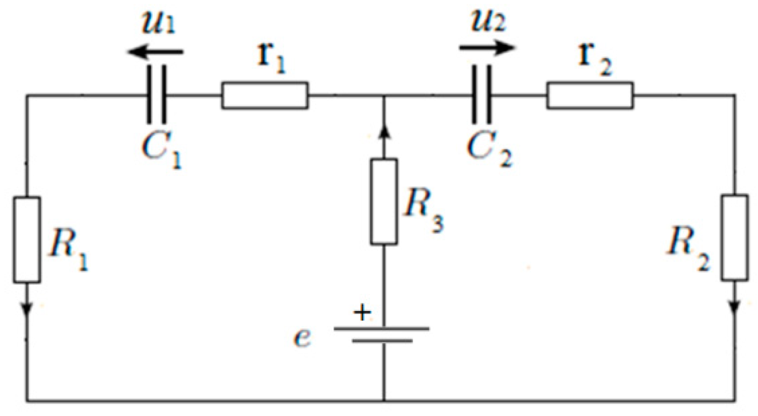
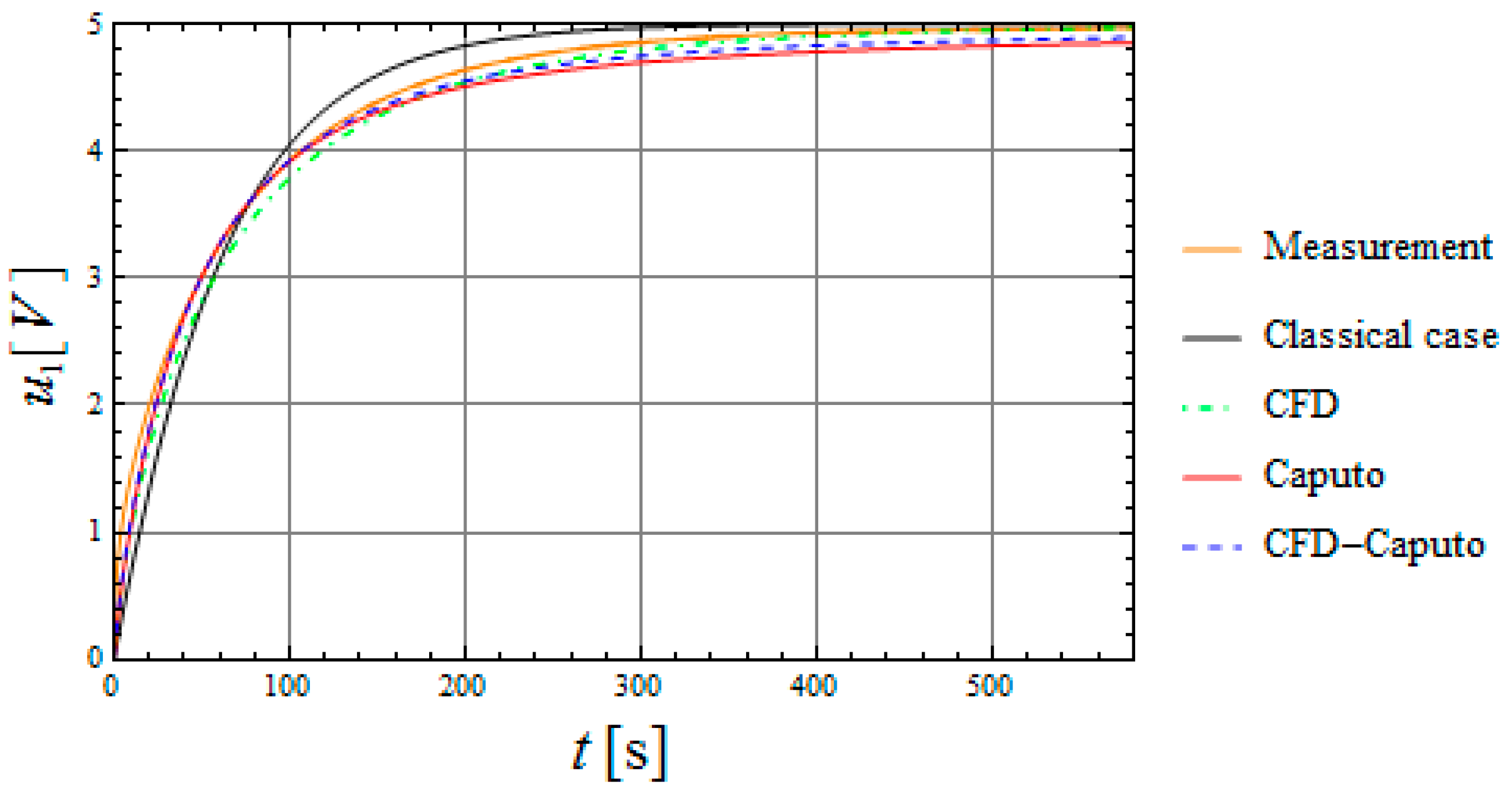
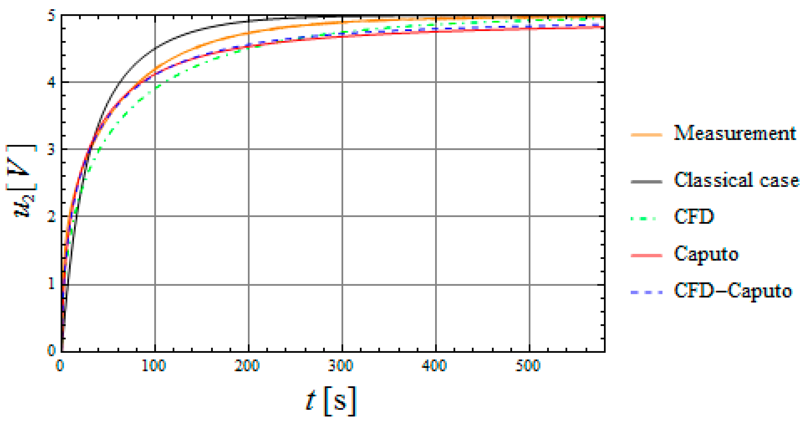
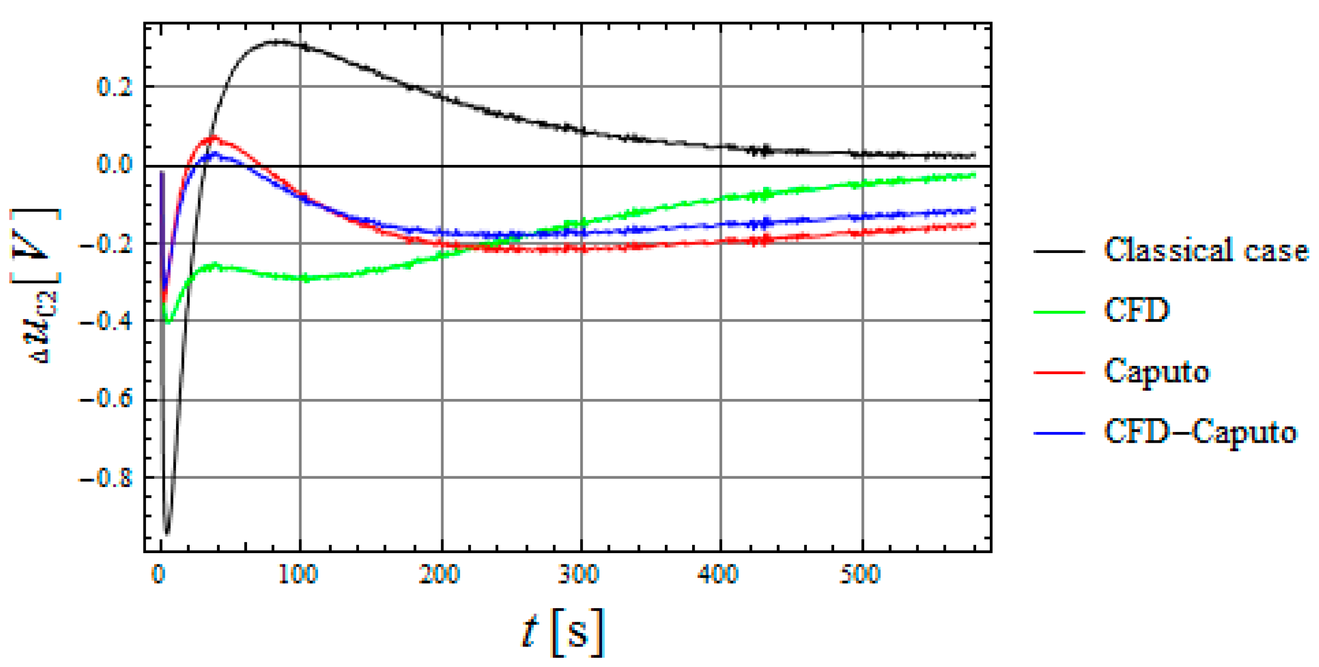
4. Fractional Electrical Circuit and General Description of the Problem

Let us consider the electrical circuit shown in Figure 1 consisting of the following elements: $e$—DC power supply, $R_1,R_2,R_3$—replaceable external resistors and two supercapacitors $C_1,C_2$ with parasitic resistance $r_1,r_2$.

The current in the supercapacitor is related to the voltage drop by the formula

$$i(t)=C_{\alpha ,\beta }{D}_t^{\alpha ,\beta }{u}_C(t)\begin{array}{c}\end{array}\mathrm{for}\begin{array}{c}\end{array}0<\alpha <1, 0<\beta \le 1,$$

(24)

where $C_{\alpha ,\beta }$ is the pseudo-capacitance in units of $F/s^{1-\alpha \beta }$. For $\alpha =\beta =1$ the Formula (24) becomes the well-known classical relation $i(t)=C\frac{d{u}_C(t)}{dt}$.

Using the Equation (24) and Kirchhoff’s laws, we may describe the transient states in the electrical circuit by the following state equation:

$$\left[\begin{array}{c}{D}_t^{{\alpha }_1,{\beta }_1}{u}_1\left(t\right)\\ D_t^{{\alpha }_2,{\beta }_2}{u}_2\left(t\right)\end{array}\right]=\left[\begin{array}{cc}{A}_{11}& A_{12}\\ A_{21}& A_{22}\end{array}\right]\left[\begin{array}{c}{u}_1\left(t\right)\\ u_2\left(t\right)\end{array}\right]+\left[\begin{array}{c}{B}_1\\ B_2\end{array}\right]e,$$

(25)

where

$$A=\left[\begin{array}{cc}{A}_{11}& A_{12}\\ A_{21}& A_{22}\end{array}\right]=\left[\begin{array}{cc}-\frac{R_3+R_2+r_2}{R^2{C}_{{\alpha }_1{\beta }_1}}& \frac{R_3}{R^2{C}_{{\alpha }_1{\beta }_1}}\\ \frac{R_3}{R^2{C}_{\alpha }{}_{{}_2{\beta }_2}}& -\frac{R_3+R_1+r_1}{R^2{C}_{\alpha }{}_{{}_2{\beta }_2}}\end{array}\right],$$

(26a)

$$B=\left[\begin{array}{c}{B}_1\\ B_2\end{array}\right]=\left[\begin{array}{c}\frac{R_2+r_2}{R^2{C}_{{\alpha }_1{\beta }_1}}\\ \frac{R_1+r_1}{R^2{C}_{{\alpha }_2{\beta }_2}}\end{array}\right],$$

(26b)

and

$$R^2=R_3\left(R_1+r_1+R_2+r_2\right)+\left(R_1+r_1\right)\left(R_2+r_2\right).$$

(26c)

The initial condition (the initial voltages across the capacitors) is given as

$$u_1\left(0\right)=u_2\left(0\right)=0.$$

(27)

The control voltage is in the form of a step function

$$e\left(t\right)=\{\begin{array}{cc}0 \mathrm{for}& t<0\\ U \mathrm{for}& t\ge 0\end{array}.$$

(28)

Using the Formula (23), we get the solution of state Equation (25) with the initial conditions (27) and control input voltage (28) in the following form:

$$x(t)=\left[F_0\left(t\right)-I_2\right]A^{-1}BU={\displaystyle \sum _{\begin{array}{l}{k}_1,k_2=0\\ k_1+k_2>0\end{array}}^{\infty }{W}_{k_1{k}_2}\frac{t^{k_1{\alpha }_1{\beta }_1+k_2{\alpha }_2{\beta }_2}}{{\beta }_1^{k_1{\alpha }_1}{\beta }_2^{k_2{\alpha }_2}}}{A}^{-1}BU,$$

(29)

where

$$\begin{array}{l}{W}_{00}=I_2,\\ W_{k_1{k}_2}=0, \mathrm{for} k_1<0 \mathrm{or} k_2<0\end{array}$$

(30a)

$$\begin{array}{l}{W}_{k_1,k_2}=\frac{\Gamma \left(\left(k_1-1\right){\alpha }_1+k_2{\alpha }_2{\beta }_2/{\beta }_1+1\right)}{\Gamma \left(k_1{\alpha }_1+k_2{\alpha }_2{\beta }_2/{\beta }_1+1\right)}{\tilde{A}}_1{W}_{k_1-1,k_2}\\ +\frac{\Gamma \left(k_1{\alpha }_1{\beta }_1/{\beta }_2+\left(k_2-1\right){\alpha }_2+1\right)}{\Gamma \left(k_1{\alpha }_1{\beta }_1/{\beta }_2+k_2{\alpha }_2+1\right)}{\tilde{A}}_2{W}_{k_1,k_2-1},\end{array}$$

(30b)

for $k_1,k_2\ge 0$ without $k_1=k_2=0$, $x(t)={[\begin{array}{cc}{u}_1(t)& u_2(t)\end{array}]}^T$ and

$${\tilde{A}}_1=\left[\begin{array}{cc}{A}_{11}& A_{12}\\ 0& 0\end{array}\right], {\tilde{A}}_2=\left[\begin{array}{cc}0& 0\\ A_{21}& A_{22}\end{array}\right].$$

(31)

In the considered circuit, resistances are $R_1=21.7 \Omega ,R_2=51.7 \Omega , R_3=98.7 \Omega ,$ internal resistances of supercapacitors $C_1$, $C_2$ are $r_1=10.44 \Omega$, $r_2=28.26 \Omega$, respectively, constant input $e=5.0 \mathrm{V}$ and initial conditions $u_1(0)=0.0 \mathrm{V}$, $u_2(0)=0.0 \mathrm{V}$. The nominal parameters of supercapacitors produced by Panasonic are $C_1=1 \mathrm{F}$ and $C_2=0.33 \mathrm{F}$ (5,5VDC, coin type, electrostatic double-layer capacitors). Since the manufacturer provides only information about capacitance, the parameters α, β and C_αβ have to be found based on measurements and fitting algorithms. Three series of measurements were taken and the average value of the results are presented in

Table 1. Estimated parameters of the supercapacitors.

	C1 (1 F)			C2 (0.33 F)
Definition	α1	β1	Cαβ1 [F/s1−αβ]	α1	β1	Cαβ2 [F/s1−αβ]
Classical case	1.000	1.000	0.911	1.000	1.000	0.211
CFD	1.000	0.761	0.424	1.000	0.761	0.091
Caputo	0.857	1.000	0.431	0.857	1.000	0.062
CFD–Caputo	0.914	0.884	0.412	0.914	0.884	0.071

.

Measurements and fitting algorithms show that the estimated parameters (Table 1) for the classical case (integer order derivative) and that given by the manufacturer are in tolerance (±30%). The values appearing in Table 1 are used to calculate the step response of the system (25) for each definition. Figure 2 and Figure 3 present the voltage measurements on the supercapacitors (sampling time of 5 ms) and the simulated step response (iteration time of 5 ms) based on the classical solution, the Conformable Fractional Derivative definition, the Caputo definition and the two-parameter Conformable Derivative in the Caputo sense. As previously, three series of measurements were taken to check the repeatability of the methodology.

Based on the measurement $u_M(t)$ and analytical (simulated) solution $u_A(t)$, we set the match error function as $\Delta u(t)=u_A(t)-u_M(t)$. Figure 4 and Figure 5 show the error function, that is, the difference between real measurement and the simulated behavior (step response based on state space solution of Equation (25) of the supercapacitors $C_1=1 \mathrm{F}$ and $C_2=0.33 \mathrm{F}$, respectively).

To present the obtained result as a number, the cumulated matching error ${\chi }^2={\displaystyle \sum _0^t\Delta u{(t)}^2}$ is given in

Table 2. Error (lower is better).

Definition	C1 (1 F)	C2 (0.33 F)
	χ2
Classical case	47.2	46.5
CFD	17.1	42.0
Caputo	22.9	35.0
CFD–Caputo	12.8	23.6

.

The Figure 4 and Figure 5 reveal that the matching error ${\chi }^2$ for the first supercapacitor was almost four times bigger for the classic solution than for the CFD–Caputo solutions, and for the second supercapacitor, two times bigger. The results given in Table 2 prove that the solution obtained for CFD in the Caputo sense gives the best results for modeling this type of dynamical system.

5. Conclusions

The solution for the two-parameters operator describing the electrical circuit containing two supercapacitors was developed. Measured characteristics (step response) of the supercapacitor were compared with theoretical results based on four definitions of derivatives: classical (integer order), the Conformable Fractional, the Caputo fractional and the two-parameter Conformable Derivative in the Caputo sense. The match error function was created. It was determined which analytical solution is best suited to describe the operation of a real electrical circuit containing fractional elements such as supercapacitors.

The measurements show that the classical approach generates the largest error in the description of the behavior of the supercapacitor. This means that this method is insufficient for describing the behavior of electrical circuits containing elements of fractional order. The fractional Caputo definition, compared to the CFD definition, allows for better description of the supercapacitor response in the initial charging phase. On the other hand, the CFD definition allows for a more accurate description in the final phase of the supercapacitor charging—close to the steady state. The advantages of both definitions were combined. Numerical simulations supported by real measurements indicate that the newly proposed CFD–Caputo definition allows for a more accurate description of the behavior of the electrical circuits with fractional elements such as supercapacitors. From Table 2 it follows that the CFD–Caputo method for a considered circuit gives 3.6 and 1.9 times more precise results than the classic approach for capacitor C₁ and C₂, respectively.

The proposed method can be extended for electrical circuits (also for mechanic circuits) containing any number of elements, but at least one should be of fractional order.

References

1. Kaczorek, T. Selected Problems in Fractional Systems Theory; Springer: Berlin, Germany, 2012. [Google Scholar]
2. Luft, M.; Szychta, E.; Nowocień, A.; Pietruszczak, D. Application of differential-integral calculus of incomplete orders in mathematical modeling of pressure transducer. Coaches. Oper. Tests 2016, 6, 972–976. (In Polish) [Google Scholar]
3. Ostalczyk, P. Epitome of Fractional Calculus: Theory and Aplications in Automatics; Lodz Technical University Publishing: Lodz, Poland, 2008. (In Polish) [Google Scholar]
4. Liouville, J. Mémoire sur quelques quéstions de géometrie et de mécanique, et sur un noveau genre pour résoudre ces quéstions. J. École Polytech. 1832, 13, 1–69. [Google Scholar]
5. Alsaedi, A.; Nieto, J.J.; Venktesh, V. Fractional electrical circuits. Adv. Mech. Eng. 2015, 7, 1–7. [Google Scholar] [CrossRef]
6. Grünwald, A.K. Über “begrenzte” Derivationen und deren anwendung. Z. Angew.Math. Phys. 1867, 12, 441–480. [Google Scholar]
7. Cioć, R. Grünwald-Letnikov derivative—Analyse in space of first order derivative. In Frontiers in Fractional Calculus, Book Series: Current Developments in Mathematical Sciences; Bentham Science Publishers Ltd.: Sharjah, United Arab Emirates, 2018; Volume 1. [Google Scholar]
8. Naeem, I.; Khan, M.D. Symmetry classification of time-fractional diffusion equation. Commun. Nonlinear Sci. Numer. Simul. 2017, 42, 560–570. [Google Scholar] [CrossRef]
9. Leo, R.A.; Sicuro, G.; Tempesta, P. A theorem on the existence of symmetries of fractional PDEs. C. R. Math. 2014, 352, 219–222. [Google Scholar] [CrossRef] [Green Version]
10. Hashemi, M.S.; Inc, M.; Bayram, M. Symmetry properties and exact solutions of the time fractional Kolmogorov-Petrovskii-Piskunov equation. Rev. Mex. Fıs. 2019, 65, 529–535. [Google Scholar] [CrossRef] [Green Version]
11. Caponetto, R.; Dongola, G.; Fortuna, L.; Petráś, I. Fractional Order Systems. Modeling and Control Applications; World Scientific: Singapoure, 2010. [Google Scholar]
12. Dzieliński, A.; Sierociuk, D. Ultracapacitor modeling and control using discrete fractional order state-space model. Acta Montan. Slovaca 2008, 13, 136–145. [Google Scholar]
13. Jesus, I.S.; Tenreiro Machado, J.A. Comparing Integer and Fractional Models in some Electrical Systems. In Proceedings of the 4th IFAC Workshop Fractional Differentiation and its Applications, Badajoz, Spain, 18–20 October 2010. [Google Scholar]
14. Kaczorek, T. Analysis of fractional electrical circuits in transient states. Logistyka 2010, 2, CD-ROM. [Google Scholar]
15. Piotrowska, E.; Rogowski, K. Analysis of fractional electrical circuit using caputo and conformable derivative definitions. In Non-Integer Order Calculus and its Applications; Ostalczyk, P., Sankowski, D., Nowakowski, J., Eds.; RRNR 2017. Lecture Notes in Electrical Engineering; Springer: Cham, Switzerland, 2019; Volume 496. [Google Scholar]
16. Sikora, R. Fractional derivatives in electrical circuit theory—Critical remarks. Arch. Electr. Eng. 2017, 66, 155–163. [Google Scholar] [CrossRef] [Green Version]
17. Yavuz, M.; Ozdemir, N. A different approach to the European option pricing model with new fractional operator. Math. Model. Nat. Phenom. 2018, 13, 1–12. [Google Scholar] [CrossRef] [Green Version]
18. Yavuz, M.; Ozdemir, N. New numerical techniques for solving fractional partial differential equations in conformable sense. In Non-Integer Order Calculus and its Applications; Ostalczyk, P., Sankowski, D., Nowakowski, J., Eds.; RRNR 2017. Lecture Notes in Electrical Engineering; Springer: Cham, Switzerland, 2019; Volume 496. [Google Scholar]
19. Yavuz, M.; Yaşkıran, B. Approximate-analytical solutions of cable equation using conformable fractional operator. New Trends Math. Sci. 2017, 4, 209–219. [Google Scholar] [CrossRef]
20. Yavuz, M.; Yaşkıran, B. Conformable derivative operator in modelling neuronal dynamics. Appl. Appl. Math. 2018, 13, 803–817. [Google Scholar]
21. Abdeljawad, T. On conformable fractional calculus. J. Comp. Appl. Math. 2015, 279, 57–66. [Google Scholar] [CrossRef]
22. İskender Eroğlu, B.B.; Avcı, D.; Özdemir, N. Optimal control problem for a conformable fractional heat conduction equation. Acta Phys. Pol. 2017, 132, 658–662. [Google Scholar] [CrossRef]
23. Khalil, R.; Al Horani, A.; Yousef, A.; Sababheh, M. A new definition of fractional derivative. J. Comput. Appl. Math. 2014, 264, 65–70. [Google Scholar] [CrossRef]
24. Martínez, L.; Rosales, J.J.; Carreño, C.A.; Lozano, J.M. Electrical circuits described by fractional conformable derivative. Int. J. Circ. Theor. Appl. 2018, 46, 1091–1100. [Google Scholar] [CrossRef]
25. Kaplan, M.; Bekir, A.; Ozer, M.N. A simple technique for constructing exact solutions to nonlinear differential equations with conformable fractional derivative. Opt. Quant. Electron. 2017, 49, 266. [Google Scholar] [CrossRef]
26. Piotrowska, E. Analysis of fractional electrical circuit with rectangular input signal using Caputo and conformable derivative definitions. Arch. Electr. Eng. 2018, 67, 789–802. [Google Scholar]
27. Piotrowska, E. Analysis of fractional electrical circuit with sinusoidal input signal using Caputo and conformable derivative definitions. Pozn. Univ. Technol. Acad. J. Electical Eng. 2019, 97, 155–167. [Google Scholar]
28. Piotrowska, E. Analysis of linear continuous-time systems by the use of the Conformable Fractional Calculus and Caputo. Arch. Electrical Eng. 2018, 67, 629–639. [Google Scholar]
29. Morales-Delgado, V.F.; Gómez-Aguilar, J.F.; Taneco-Hernandez, M.A. Analytical solutions of electrical circuits described by fractional conformable derivatives in Liouville-Caputo sense. Int. J. Electron. Commun. 2018, 85, 108–117. [Google Scholar] [CrossRef]
30. Piotrowska, E. Positive continuous—Time linear electrical circuit. Pozn. Univ. Technol. Acad. J. Electical Eng. 2018, 93, 299–309. [Google Scholar] [CrossRef]
31. Kaczorek, T.; Rogowski, K. Fractional Linear Systems and Electrical Circuits; Springer: Cham, Switzerland, 2014. [Google Scholar]
32. AbdelAty, A.M.; Radwan, A.G.; Ahmed, W.A.; Faied, M. Charging and discharging RCα circuit under Riemann-Liouville and Caputo fractional derivatives. In Proceedings of the 13th International Conference on Electrical Engineering/Electronics, Computer, Telecommunications and Information Technology (ECTI-CON), Chiang Mai, Thailand, 28 June–1 July 2016; pp. 1–4. [Google Scholar]
33. Jiang, Y.; Zhang, B. Comparative study of riemann–liouville and caputo derivative definitions in time-domain analysis of fractional-order capacitor. IEEE Trans. Circuits Syst. II Express Briefs 2020, 67, 2184–2188. [Google Scholar] [CrossRef]
34. Elwakil, A.S.; Radwan, A.G.; Freeborn, T.J.; Allagui, A.; Maundy, B.J.; Fouda, M. Low-voltage commercial super-capacitor response to periodic linear-with-time current excitation: A case study. IET Circuits Devices Syst. 2017, 11, 189–195. [Google Scholar] [CrossRef]
Figure 1. RC electrical circuit with supercapacitor (source: own).
Symmetry 13 00771 g001
Figure 2. Measured and simulated step response for capacitor C 1 .
Symmetry 13 00771 g002
Figure 3. Measured and simulated step response for capacitor C 2 .
Symmetry 13 00771 g003
Figure 4. Matching error function for first capacitor C 1 = 1   F .
Symmetry 13 00771 g004
Figure 5. Matching error function for first capacitor C 2 = 0.33   F .
Symmetry 13 00771 g005